A Guide to MATLAB for Chemical Engineering Problem Solving phần 1 docx

A Guide to MATLAB
for Chemical Engineering Problem Solving
(ChE465 Kinetics and Reactor Design)
Kip D. Hauch
Dept. of Chemical Engineering
University of Washington
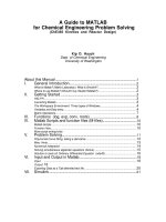
About this Manual 1
I. General Introduction 2
What is Matlab? (Matrix Laboratory), What is Simulink? 2
Where to use Matlab? (Should I buy Student Matlab?) 2
II. Getting Started 3
HELP!!! 3
Launching Matlab 3
The Workspace Environment Three types of Windows 4
Variables and Data entry 4
Matrix Operations 7
III. Functions (log, exp, conv, roots) 8
IV. Matlab Scripts and function files (M-files) 10
Matlab Scripts 10
Function files 10
More script writing hints
V. Problem Solving 11
Polynomial Curve fitting, taking a derivative 12
Misc. Hints 13
Numerical Integration 14
Solving simultaneous algebraic equations (fsolve) 15
Solution to (sets of) Ordinary Differential Equation (ode45) 16
VI. Input and Output in Matlab 18
Input 18
Output 18
Exporting Data as a Tab-delimited text file 20

VII. Simulink 21
About this Manual
Matlab is a matrix-based mathematical software package that is used in several
ChE classes including ChE465, Kinetics and Reactor Design, ChE480 Process
Control& Laboratory, and ChE475 Computational Methods. It may also be useful
in ChE310 as well as other ChE and other courses e.g. P-Chem. While Matlab is
very powerful, many students often find it to be "unfriendly" and difficult to
learn and understand; and frankly it is. This manual was compiled from
several handouts that have been used previously in the above classes in an
effort to make Matlab easier for you to understand and use. This manual
demonstrates a select assortment of the common features and functions that
you will use in your ChE classes. IT is NOT meant to be comprehensive, rather
it is meant to supplement the published Matlab manual (Student Matlab,
available at the UW Bookstore or with the purchase of the Student Matlab
software.), and the on-line help available in Matlab (See p. 3) Another good
reference is Engineering Problem Solving using Matlab, by D.M. Etter
(Prentice Hall, 1993.)
This manual assumes that you are already familiar with the typical Macintosh
operating system and the environment common to most Macintosh
applications. Along with scalar variables, Matlab makes extensive use of
vectors and matrices, and familiarity with the standard vector and matrix
operations is very helpful in understanding how Matlab works.

This manual was compiled in Fall 1994 and includes material form Profs:
Krieger-Brockett, Holt, Ricker, and Finlayson. If you find errors or wish to
suggest changes or inclusions please contact your course instructor.
Matlab Guide: ChE465
KDH v.2.1.1 p. 2 Print date: 10/4/00
WHAT IS MATLAB? (MATRIX LABORATORY), WHAT IS SIMULINK?
It is a powerful mathematical software package that you may use in solving

some of the problems assigned in this course. M
ATLAB will likely be used
again (more heavily) when you take ChE480 Process Control, and may also b e
helpful to you in other coursework or experimental work as well.
As with any software, it is only a tool that you may choose to apply to solve
particular problems or tasks. It will not interpret problems for you; it will n ot
guarantee that you get the 'right' answer. M
ATLAB IS only as smart (or as
dumb) as the person using it. During your coursework you will encounter
tasks such as numerical integration, and differential equation solving.
M
ATLAB is not the only software tool that you may choose to apply to solve
these tasks; other packages such as Mathematica, Maple V, Theorist, MathCAD
and others may be adept at meeting your needs. In the future, as a fully
employed process engineer you will be given certain mathematical tasks to
solve, and you may be requested to adapt to using the software tools (and
platforms) provided. At the UW we will make available the Macintosh version
of Matlab for your use; but you should feel free to use other software tools o r
platforms if you are comfortable with them. We will, however, be unable to
help you with other packages besides Matlab for Macintosh.
Part of the power of Matlab comes from the fact that one can manipulate
and operate on scalars, vectors and matrices with the same level of ease.
However, therein lies one pitfall; the user must pay close attention to whether
Matlab is assuming a particular variable to be a scalar, row vector, column
vector, or matrix. Matlab does nothing to make this distinction immediately
apparent.
Matlab also provides for a powerful high-level programming or scripting
language. There exist hundreds of pre-written subroutines that accomplish
simple to very high level mathematical manipulations, such as matrix
inversion, ordinary differential equation solving, numerical integration, etc.

In fact, most of the powerful commands that you invoke from within Matlab
are actually separately written subroutines. You can (and will) write your
own subroutines, as well as examine the ones the manufacturer has provided.
Simulink (previously known as Simulab) is a graphical interface for
Matlab that links together blocks of complicated Matlab code to perform
analysis, modeling, and simulation of dynamic systems. Simulink is used in t h e
Process Control course for process control diagrams. At various times you may
see Matlab referred to as: Matlab, Matlab/S, Matlab/Simulink, or just Simulink.
Don't let this confuse you, in each case you are still using Matlab.
WHERE TO USE MATLAB? (SHOULD I BUY STUDENT MATLAB?)
The Macintosh version of MATLAB is available for your use in Benson Hall
Computing Lab, Room 125. This computer laboratory is for the use of students
enrolled in ChE classes only; it is not open to the general campus. Our
computer resources are limited, and the computer lab is reserved at certain
times during the week for instructional use. Budget your time accordingly
(i.e. plan ahead, work during non-peak hours). The M
ATLAB application
A Guide to MATLAB
for Chemical Engineering Problem Solving
(ChE465 Kinetics and Reactor Design)
I. GENERAL INTRODUCTION
There are two easy
ways to tell if a
variable is a scalar,
vector or matrix: 1)
use the Who&Size
command by typing
whos at the
command line
prompt, or 2) simply

type the variable
name and return.
Matlab responds by
displaying the
variable and it's
current value(s)
Matlab Guide: ChE465
KDH v.2.1.1 p. 3 Print date: 10/4/00
cannot be copied to your own machine.
The version of M
ATLAB available in the computing lab is a complete, full-
featured
Matlab Guide: ChE465
KDH v.2.1.1 p. 4 Print date: 10/4/00
version of MATLAB (Matlab Professional vers. 4.2a). The publishers of Matlab
have made available a somewhat limited version of the program, Student
M
ATLAB, available for individual purchase at a reasonable cost. The biggest
limitation is that the Student version is limited to working with variables
(matrices) with less than 8K of elements (8192 elements or a 32 by 32 matrix).
Student Matlab therefore, can handle only smaller problems, and may r u n
more slowly. Also, some of the graphics and output routines may be more
limited. It is likely that Student M
ATLAB will handle many, but not all of t he


problems you will want to tackle while here at UW ChE. As with any software I
urge you to talk with other classmates who may have purchased Student
M
ATLAB, and try the software for yourself. You will have to weigh many

factors, such as the cost, the convenience to you of having your own copy,
your own computer hardware and its performance, and the limitations of the
Student version, before making your purchase decision.
(Student) M
ATLAB is also available on the MS-DOS platform as well as o ther
workstation and mainframe platforms, however, you will be on your own
regarding questions specific to these other platforms.
M
ATLAB has simple and fairly extensive on-line help, although it is, a t
times, cryptic. You will be expected to use the on-line help to first learn
about the syntax of a particular command or function, and to refresh your
memory later. In this tutorial, you should first try to read through the on-line
help for the applicable commands, then try the examples. If you are still
stuck, re-read the on-line help, and then seek help from your instructor or TA.
On-line help is available by selecting About Matlab (or About Simulink)
from the pulldown
 menu. Matlab also provides several demos here that you
should explore.
On-line help is also available from the command prompt by simply typing:
» help function name
This is the easiest way to get help, and can be used at any time in the COMMAND
window.
Launching Matlab
All students are responsible for establishing an 'account' on the ChE UGrad
Appleshare server, and abiding by the rules and regulations regarding the use
of the computers and software. If you do not yet have such an account, or if
you have forgotten how to use it, or if you have forgotten your password; g o
see the Department's Computer Engineer, Eric Mehan, in room B-007
immediately. The UGrad server provides you with access to a variety of
applications including Word, Excel, DeltaGraphPro, as well as access to campus

mainframes, e-mail etc. You are also provided with a small storage space o n
the server where you may store your own personal work files.
II. GETTING STARTED
HELP!!!
(Getting on-line
Help)
IMPORTANT
STUFF ➨
Matlab Guide: ChE465
KDH v.2.1.1 p. 5 Print date: 10/4/00
THE FIRST TIME YOU LAUNCH MATLAB: Establish a connection to the UGrad
server. COPY the file MATLAB from the Application Startup Documents folder
on the Macintosh hard drive to your personal folder on the server. (Rename it
Matlab Startup) You may now launch Matlab at any time by double clicking o n
this startup document in your folder. By launching Matlab in this manner, it
will by default save your work files to your folder on the Server. After you
have saved your work to your folder on the server, you may copy your files to
a floppy for transport home, or just for use as a backup. You must pay careful
attention to where Matlab is saving your files (which disk, server, directory,
etc.). Matlab must be 'pointed' in the right direction, especially if you expect it
to call a function or subroutine that you have written and saved in a particular
location on the server. Also, you may lose your work if you accidently save to
a folder or area to which you have no access. Most importantly: NEVER SAVE
YOUR FILES ON THE MACINTOSH HARD DISK. As part of routine maintenance,
the hard disks on the Macintoshs are frequently erased completely WITHOUT
PRIOR WARNING.
The Workspace Environment Three types of Windows
The Matlab environment provides three different types of windows: t h e
COMMAND window, M-FILE editing windows and FIGURE windows. Each type of
window is used for a different purpose, and it is important that you keep track

of which window is your 'active' window. Use the
WINDOW pull down menu to
conveniently switch between any of the open windows. The startup document
leads to an M-FILE window. You should simply close this window without
saving any changes.
In the COMMAND window, Matlab executes the commands on each line as
you type them in at the command prompt, ». You will use this window to input
values for variables and execute short series of commands. Matlab also
displays most numerical results in this window. You may use the familiar Cut
and Paste while in the COMMAND window as well as the mouse to perform
editing.
Matlab outputs graphical data such as plots to a FIGURE window. A figure
window will be created automatically when you issue a graphical output
command, like
plot. However, often the figure widow that is created is buried
behind other windows. Plots can be copied and imported into other documents
as graphics in the usual manner.
Since typing even a handful of the same commands over and over again is
tiresome, Matlab provides for powerful scripting of macros. The script file
(called a M-file) is simply a list of commands. When the script file is executed,
it is as if each of the commands was entered at the command prompt in t he
COMMAND window for you. The M-FILE Window is used to build, edit, a nd
execute these scripts or programs. This window operates in the same manner
as a simple text editor. Writing M-Files is discussed later in section IV.
Variables and Data entry
Once Matlab is launched you may begin defining variables at will. Each
variable will remain stored in memory, with its assigned value until: it is
reassigned a new value, it is manually cleared, or you quit Matlab. Although
you can name variables almost anything, here are some tips. Matlab is case
sensitive ('A' is not the same as 'a'). For this reason, you

may find it more convenient to avoid using lots of capital letters. Stick to
alphanumeric characters and the underbar. Keep your variable names short,
but still long enough to be descriptive and easily distinguishable. (In scripts
you should use comment lines to clearly spell out the meaning of t he
variables.) The default font used by Matlab is Monoco 12pt. In this font t h e
capital letter 'Oh" and the Zero are identical: beware.
Never save
your files to
the Macintosh
hard disk.
Save your
work
frequently.
Backup your
work on
floppy and
take it with
you.
+
TIP: Use the
WINDOW pull down
menu to keep
track of, and
access open
windows of all
types.
+ TIP: In the
COMMAND Window,
Use the Up arrow
and Down arrow on

the keyboard to
scroll through your
most recently issued
commands.
+ TIP: The first
step in writing a
script is to open a
new M-file window.
+ TIP: Matlab is
case sensitive ('A'
is not the same as
'a')
Matlab Guide: ChE465
KDH v.2.1.1 p. 6 Print date: 10/4/00
Assigning a scalar to a variable is straightforward:
»a = 5.348
a =
5.3480
»
If you perform no other operations, Matlab responds by echoing back the
variable with the value assigned.
Entering a vector or matrix is performed using a variable name and t he
square brackets. The individual elements may be separated by spaces or b y
commas. New rows may be indicated by returns or by semi-colons (;) within
the brackets. Finally if no variable name is specified, Matlab assigns the input
to the variable
ans by default — you should avoid using ans as a variable name
in your scripts.
Matlab Guide: ChE465
KDH v.2.1.1 p. 7 Print date: 10/4/00

Examples:
»a = [1 2 3]
a =
1 2 3
»b = [1;2;3]
b =
1
2
3
»[ 1 3 5
2 4 6
3 6 9]
ans =
1 3 5
2 4 6
3 6 9
Exercise:
Input the following matrices::
123
538
2.3 5.6 10
,
123
100
105
There are several useful shortcuts for building more complex matrices.
First the colon operator can be used to assign an evenly spaced range of
values. The usage is:
[starting value : increment : end value]. If no increment is specified it is
assumed to be one.

Example:
»time = [0: 0.1 :1.5]
time =
Columns 1 through 7
0 0.1000 0.2000 0.3000 0.4000 0.5000 0.6000
Columns 8 through 14
0.7000 0.8000 0.9000 1.0000 1.1000 1.2000 1.3000
Columns 15 through 16
1.4000 1.5000
Individual elements or subsets of a matrix can be freely referred to by their
indices
a(row, column).
Examples:
»a = [1 2 3; 4 5 6; 7 8 9]
a =
1 2 3
4 5 6
7 8 9
+ TIP: Assigning a
range of values
within a vector
without typing
each element.
+ TIP: Append a
semi-colon (;) to
the end of the
line before the
return to
suppress this
kind of lengthy

output.
Matlab Guide: ChE465
KDH v.2.1.1 p. 8 Print date: 10/4/00
»a(2,3)
ans =
6
»a(1:2,3)
ans =
3
6
note the use of the colon operator to specify a range
»conc = [1 .9 .8 .7 .65 .63
2 1.9 1.8 1.6 1.5 1.43
2 .9 .85 .8 .75 .71]
conc =
1.0000 0.9000 0.8000 0.7000 0.6500 0.6300
2.0000 1.9000 1.8000 1.6000 1.5000 1.4300
2.0000 0.9000 0.8500 0.8000 0.7500 0.7100
»conc(:,6)
says conc('all rows',column#6)
ans =
0.6300
1.4300
0.7100
Finally, here are some special matrices that are often useful
»eye(3) The identity matrix yields
ans =
1 0 0
0 1 0
0 0 1

»ones(2,4)
Fills in a matrix of specified size with ones
ans =
1 1 1 1
1 1 1 1
»zeros(2,3)
likewise with zeros
ans =
0 0 0
0 0 0
+ TIP: Extract a
row or column
from a data
matrix
Matlab Guide: ChE465
KDH v.2.1.1 p. 9 Print date: 10/4/00
Larger Matrices can be built from smaller ones.
Example:
a =
1 2 3
4 5 6
7 8 9
»e = [[zeros(2,3);ones(1,3)] a]
e =
0 0 0 1 2 3
0 0 0 4 5 6
1 1 1 7 8 9
»e = [e e]
e =
0 0 0 1 2 3 0 0 0 1 2 3

0 0 0 4 5 6 0 0 0 4 5 6
1 1 1 7 8 9 1 1 1 7 8 9
Matrix Operations
»a = [1 2 3
4 5 6
7 8 9]
a =
1 2 3
4 5 6
7 8 9
»a + a
ans =
2 4 6
8 10 12
14 16 18
»a * a
matrix multiplication
ans =
30 36 42
66 81 96
102 126 150
Placing a period in front of the
operator causes it to be executed
on a
element-by-element basis.
»a .* a
ans =
1 4 9
16 25 36
49 64 81

There are two matrix division
symbols in Matlab, / and \ . a/b =
a*inv(b)
and a\b = inv(a)*b.
»a = [1 2 5
2 3 1
3 1 6]
a =
1 2 5
2 3 1
3 1 6
»b = [1 1 5
4 1 2
6 4 1]
b =
1 1 5
4 1 2
IMPORTANT
➨
+ TIP:Pay close
attention to
whether your
variables are row
or column vectors
Matlab Guide: ChE465
KDH v.2.1.1 p. 10 Print date: 10/4/00
6 4 1
»a/b
ans =
1.1569 -0.5686 0.3529

0.3922 -0.9216 0.8824
0.9216 0.7843 -0.1765
»a\b
ans =
2.4722 1.1667 -1.6111
-0.2500 -0.5000 1.5000
-0.1944 0.1667 0.7222
And again, the element - by -
element operator.
»a./b
ans =
1.0000 2.0000 1.0000
0.5000 3.0000 0.5000
0.5000 0.2500 6.0000
The transpose is represented by th e
apostrophe.
»a = [1 2 3
4 5 6
7 8 9]
a =
1 2 3
4 5 6
7 8 9
»a'
ans =
1 4 7
2 5 8
3 6 9
»t = [0:8]
t =

0 1 2 3 4 5 6 7 8
»t = t'
t =
0
1
2
3
4
5
6
7
8

Matlab is complete with a large number of useful, specialized, built-in
functions. Descriptions of each function can be displayed using the on-line
help. Here are some more commonly used functions:
The natural logarithm in Matlab is performed using the command:

log(x)
The base-10 logarithm is performed using the command
log10(x), and the exponential is exp(x).
Polynomial multiplication using convolve: (see also deconv)
What is:
(3X
2
+ 2X + 5) * (19X
2
- 7X - 13) ?
Solution:
»a = [3 2 5] (Put the polynomial coefficients into a

III. FUNCTIONS (log, exp, conv, roots)
+ NOTE:: The
natural logarithm

is log(x) not
ln(x)
Matlab Guide: ChE465
KDH v.2.1.1 p. 11 Print date: 10/4/00
row vector in decreasing power)


a =
3 2 5
»b = [19 -7 -13]
b =
19 -7 -13
»conv(a,b)
ans =
57 17 42 -61 -65
Answer:
57X
4
+ 17X
3
+ 42X
2
- 61X - 65
Exercise:
What is
(3X

3
+ 2X + 5) * (X
3
+ 2X
2
- 2) ?
answer:
3X
6
+ 6X
5
+ 2X
4
+ 3X
3
+ 10X
2
- 4X + 10.
The roots of a polynomial can be found from its coefficients, e.g.:
What are the roots of:
5X
2
+ 17X + 6 ?
»roots([5 17 6])
ans =
-3.0000
-0.4000
What are the roots of
5X
2

+ 6.5X + 19 ?
»roots([5 6.5 19])
ans =
-0.6500 + 1.8378i
-0.6500 - 1.8378i
The roots are complex.