David G. Luenberger, Yinyu Ye - Linear and Nonlinear Programming International Series Episode 1 Part 6 pptx
Bạn đang xem bản rút gọn của tài liệu. Xem và tải ngay bản đầy đủ của tài liệu tại đây (403.99 KB, 25 trang )
∗
5.3 The Ellipsoid Method 115
form. The system has m =3 equations and n =6 nonnegative variables. It can be
verified that it takes 2
3
−1 =7 pivot steps to solve the problem with the simplex
method when at each step the pivot column is chosen to be the one with the largest
(because this a maximization problem) reduced cost. (See Exercise 1.)
The general problem of the class (1) takes 2
n
−1 pivot steps and this is in fact
the number of vertices minus one (which is the starting vertex). To get an idea of
how bad this can be, consider the case where n =50. We have 2
50
−1 ≈10
15
In
a year with 365 days, there are approximately 3 ×10
7
seconds. If a computer ran
continuously, performing a million pivots of the simplex algorithm per second, it
would take approximately
10
15
3×10
7
×10
6
≈33 years
to solve a problem of this class using the greedy pivot selection rule.
∗
5.3 THE ELLIPSOID METHOD
The basic ideas of the ellipsoid method stem from research done in the 1960s and
1970s mainly in the Soviet Union (as it was then called) by others who preceded
Khachiyan. In essence, the idea is to enclose the region of interest in ever smaller
ellipsoids.
The significant contribution of Khachiyan was to demonstrate in that under
certain assumptions, the ellipsoid method constitutes a polynomially bounded
algorithm for linear programming.
The version of the method discussed here is really aimed at finding a point of
a polyhedral set given by a system of linear inequalities.
=y ∈ E
m
y
T
a
j
≤c
j
j=1n
Finding a point of can be thought of as equivalent to solving a linear programming
problem.
Two important assumptions are made regarding this problem:
(A1) There is a vector y
0
∈E
m
and a scalar R>0 such that the closed ball Sy
0
R
with center y
0
and radius R, that is
y ∈E
m
y −y
0
≤R
contains .
(A2) If is nonempty, there is a known scalar r>0 such that contains a ball
of the form Sy
∗
r with center at y
∗
and radius r. (This assumption implies
that if is nonempty, then it has a nonempty interior and its volume is at
least volS0 r)
2
.
2
The (topological) interior of any set is the set of points in which are the centers of
some balls contained in .
116 Chapter 5 Interior-Point Methods
Definition. An ellipsoid in E
m
is a set of the form
E =y ∈E
m
y −z
T
Qy −z ≤1
where z ∈E
m
is a given point (called the center) and Q is a positive definite
matrix (see Section A.4 of Appendix A) of dimension m ×m. This ellipsoid is
denoted ellz Q.
The unit sphere S0 1 centered at the origin 0 is a special ellipsoid with Q =I,
the identity matrix.
The axes of a general ellipsoid are the eigenvectors of Q and the lengths of the
axes are
−1/2
1
−1/2
2
−1/2
m
, where the
i
’s are the corresponding eigenvalues.
It can be shown that the volume of an ellipsoid is
volE =volS0 1
m
i=1
−1/2
i
=volS0 1detQ
−1/2
Cutting Plane and New Containing Ellipsoid
In the ellipsoid method, a series of ellipsoids E
k
is defined, with centers y
k
and
with the defining Q =B
−1
k
where B
k
is symmetric and positive definite.
At each iteration of the algorithm, we have ⊂E
k
. It is then possible to check
whether y
k
∈ If so, we have found an element of as required. If not, there is
at least one constraint that is violated. Suppose a
T
j
y
k
>c
j
Then
⊂
1
2
E
k
=y ∈E
k
a
T
j
y ≤a
T
j
y
k
This set is half of the ellipsoid, obtained by cutting the ellipsoid in half through its
center.
The successor ellipsoid E
k+1
is defined to be the minimal-volume ellipsoid
containing 1/2E
k
. It is constructed as follows. Define
=
1
m +1
=
m
2
m
2
−1
=2
y
k
1/2 E
Fig. 5.1 A half-ellipsoid
∗
5.3 The Ellipsoid Method 117
Then put
y
k+1
=y
k
−
a
T
j
B
k
a
j
1/2
B
k
a
j
B
k+1
=
B
k
−
B
k
a
j
a
T
j
B
k
a
T
j
B
k
a
j
(2)
Theorem 1. The ellipsoid E
k+1
= elly
k+1
B
−1
k+1
defined as above is the
ellipsoid of least volume containing 1/2E
k
. Moreover,
volE
k+1
volE
k
=
m
2
m
2
−1
m−1/2
m
m +1
< exp
−
1
2m +1
< 1
Proof. We shall not prove the statement about the new ellipsoid being of least
volume, since that is not necessary for the results that follow. To prove the remainder
of the statement, we have
volE
k+1
volE
k
=
detB
1/2
k+1
detB
1/2
k
For simplicity, by a change of coordinates, we may take B
k
= I Then B
k+1
has
m −1 eigenvalues equal to =
m
2
m
2
−1
and one eigenvalue equal to −2 =
m
2
m
2
−1
1−
2
m+1
=
m
m+1
2
The reduction in volume is the product of the square roots
of these, giving the equality in the theorem.
Then using 1+x
p
e
xp
, we have
m
2
m
2
−1
m−1/2
m
m +1
=
1+
1
m
2
−1
m−1/2
1−
1
m +1
< exp
1
2m +1
−
1
m +1
=exp
−
1
2m +1
Convergence
The ellipsoid method is initiated by selecting y
0
and R such that condition (A1) is
satisfied. Then B
0
= R
2
I, and the corresponding E
0
contains . The updating of
the E
k
’s is continued until a solution is found.
Under the assumptions stated above, a single repetition of the ellipsoid method
reduces the volume of an ellipsoid to one-half of its initial value in Om iterations.
(See Appendix A for O notation.) Hence it can reduce the volume to less than that
of a sphere of radius r in Om
2
logR/r iterations, since its volume is bounded
118 Chapter 5 Interior-Point Methods
from below by volS0 1r
m
and the initial volume is volS0 1R
m
. Generally
a single iteration requires Om
2
arithmetic operations. Hence the entire process
requires Om
4
logR/r arithmetic operations.
3
Ellipsoid Method for Usual Form of LP
Now consider the linear program (where A is m×n)
P
maximize c
T
x
subject to Ax ≤b
x ≥0
and its dual
D
minimize y
T
b
subject to y
T
A ≥c
T
y ≥0
Both problems can be solved by finding a feasible point to inequalities
−c
T
x +b
T
y ≤0
Ax ≤b
−A
T
y ≤−c
x y ≥0
(3)
where both x and y are variables. Thus, the total number of arithmetic operations
for solving a linear program is bounded by Om+n
4
logR/r.
5.4 THE ANALYTIC CENTER
The new interior-point algorithms introduced by Karmarkar move by successive
steps inside the feasible region. It is the interior of the feasible set rather than the
vertices and edges that plays a dominant role in this type of algorithm. In fact, these
algorithms purposely avoid the edges of the set, only eventually converging to one
as a solution.
Our study of these algorithms begins in the next section, but it is useful at this
point to introduce a concept that definitely focuses on the interior of a set, termed
the set’s analytic center. As the name implies, the center is away from the edge.
In addition, the study of the analytic center introduces a special structure,
termed a barrier or potential that is fundamental to interior-point methods.
3
Assumption (A2) is sometimes too strong. It has been shown, however, that when the data
consists of integers, it is possible to perturb the problem so that (A2) is satisfied and if the
perturbed problem has a feasible solution, so does the original .
5.4 The Analytic Center 119
Consider a set in a subset of of E
n
defined by a group of inequalities as
=x ∈ g
j
x 0j=1 2m
and assume that the functions g
j
are continuous. has a nonempty interior
=
x ∈ g
j
x>0 all j Associated with this definition of the set is the potential
function
x =−
m
j=1
log g
j
x
defined on
The analytic center of is the vector (or set of vectors) that minimizes the
potential; that is, the vector (or vectors) that solve
min x =min
−
m
j=1
logg
j
xx ∈g
j
x>0 for each j
Example 1. (A cube). Consider the set defined by x
i
01 −x
i
0 for
i = 1 2n. This is = 0 1
n
, the unit cube in E
n
. The analytic center can
be found by differentiation to be x
i
= 1/2 for all i. Hence, the analytic center is
identical to what one would normally call the center of the unit cube.
In general, the analytic center depends on how the set is defined—on the
particular inequalities used in the definition. For instance, the unit cube is also
defined by the inequalities x
i
01−x
i
d
0 with d>1 In this case the solution
is x
i
= 1/d +1 for all i. For large d this point is near the inner corner of the
unit cube.
Also, the additional of redundant inequalities can also change the location
of the analytic center. For example, repeating a given inequality will change the
center’s location.
There are several sets associated with linear programs for which the analytic
center is of particular interest. One such set is the feasible region itself. Another is
the set of optimal solutions. There are also sets associated with dual and primal-dual
formulations. All of these are related in important ways.
Let us illustrate by considering the analytic center associated with a bounded
polytope in E
m
represented by n>mlinear inequalities; that is,
=y ∈ E
m
c
T
−y
T
A 0
where A ∈ E
m×n
and c ∈E
n
are given and A has rank m. Denote the interior of
by
=y ∈E
m
c
T
−y
T
A > 0
120 Chapter 5 Interior-Point Methods
The potential function for this set is
y ≡−
n
j=1
logc
j
−y
T
a
j
=−
n
j=1
logs
j
(4)
where s ≡ c−A
T
y is a slack vector. Hence the potential function is the negative
sum of the logarithms of the slack variables.
The analytic center of is the interior point of that minimizes the potential
function. This point is denoted by y
a
and has the associated s
a
= c −A
T
y
a
. The
pair y
a
s
a
is uniquely defined, since the potential function is strictly convex (see
Section 7.4) in the bounded convex set .
Setting to zero the derivatives of y with respect to each y
i
gives
n
j=1
a
ij
c
j
−y
T
a
j
=0 for all i
which can be written
n
j=1
a
ij
s
j
=0 for all i
Now define x
j
=1/s
j
for each j. We introduce the notion
x s ≡x
1
s
1
x
2
s
2
x
n
s
n
T
which is component multiplication. Then the analytic center is defined by the
conditions
x s =1
Ax =0
A
T
y +s =c
The analytic center can be defined when the interior is empty or equalities are
present, such as
=y ∈ E
m
c
T
−y
T
A 0 By =b
In this case the analytic center is chosen on the linear surface y By = b to
maximize the product of the slack variables s = c −A
T
y. Thus, in this context
the interior of refers to the interior of the positive orthant of slack variables:
R
n
+
≡s s 0. This definition of interior depends only on the region of the slack
variables. Even if there is only a single point in with s = c −A
T
y for some y
where By = b with s > 0, we still say that
is not empty.
5.5 The Central Path 121
5.5 THE CENTRAL PATH
The concept underlying interior-point methods for linear programming is to use
nonlinear programming techniques of analysis and methodology. The analysis is
often based on differentiation of the functions defining the problem. Traditional
linear programming does not require these techniques since the defining functions
are linear. Duality in general nonlinear programs is typically manifested through
Lagrange multipliers (which are called dual variables in linear programming). The
analysis and algorithms of the remaining sections of the chapter use these nonlinear
techniques. These techniques are discussed systematically in later chapters, so rather
than treat them in detail at this point, these current sections provide only minimal
detail in their application to linear programming. It is expected that most readers
are already familiar with the basic method for minimizing a function by setting
its derivative to zero, and for incorporating constraints by introducing Lagrange
multipliers. These methods are discussed in detail in Chapters 11–15.
The computational algorithms of nonlinear programming are typically iterative
in nature, often characterized as search algorithms. At any step with a given point,
a direction for search is established and then a move in that direction is made to
define the next point. There are many varieties of such search algorithms and they
are systematically presented throughout the text. In this chapter, we use versions of
Newton’s method as the search algorithm, but we postpone a detailed study of the
method until later chapters.
Not only have nonlinear methods improved linear programming, but interior-
point methods for linear programming have been extended to provide new
approaches to nonlinear programming. This chapter is intended to show how
this merger of linear and nonlinear programming produces elegant and effective
methods. These ideas take an especially pleasing form when applied to linear
programming. Study of them here, even without all the detailed analysis, should
provide good intuitive background for the more general manifestations.
Consider a primal linear program in standard form
LP minimize c
T
x (5)
subject to Ax =b
x 0
We denote the feasible region of this program by
p
. We assume that
p
= x
Ax =b x > 0 is nonempty and the optimal solution set of the problem is bounded.
Associated with this problem, we define for 0 the barrier problem
BP minimize c
T
x −
n
j=1
logx
j
(6)
subject to Ax =b
x > 0
122 Chapter 5 Interior-Point Methods
It is clear that = 0 corresponds to the original problem (5). As →, the
solution approaches the analytic center of the feasible region (when it is bounded),
since the barrier term swamps out c
T
x in the objective. As is varied continuously
toward 0, there is a path x defined by the solution to (BP). This path x is
termed the primal central path.As →0 this path converges to the analytic center
of the optimal face x c
T
x = z
∗
Ax = b x 0 where z
∗
is the optimal value
of (LP).
A strategy for solving (LP) is to solve (BP) for smaller and smaller values
of and thereby approach a solution to (LP). This is indeed the basic idea of
interior-point methods.
At any >0, under the assumptions that we have made for problem (5), the
necessary and sufficient conditions for a unique and bounded solution are obtained
by introducing a Lagrange multiplier vector y for the linear equality constraints to
form the Lagrangian (see Chapter 11)
c
T
x −
n
j=1
logx
j
−y
T
Ax −b
The derivatives with respect to the x
j
’s are set to zero, leading to the conditions
c
j
−/x
j
−y
T
a
j
=0 for each j
or equivalently
X
−1
1+A
T
y =c
(7)
where as before a
j
is the j-th column of A 1 is the vector of 1’s, and X is
the diagonal matrix whose diagonal entries are the components of x > 0. Setting
s
j
=/x
j
the complete set of conditions can be rewritten
x s =1
Ax =b
A
T
y +s =c
(8)
Note that y is a dual feasible solution and c−A
T
y > 0 (see Exercise 4).
Example 2. (A square primal). Consider the problem of maximizing x
1
within
the unit square =0 1
2
The problem is formulated as
min −x
1
subject to x
1
+x
3
=1
x
2
+x
4
=1
x
1
0x
2
0x
3
0x
4
0
5.5 The Central Path 123
Here x
3
and x
4
are slack variables for the original problem to put it in standard
form. The optimality conditions for x consist of the original 2 linear constraint
equations and the four equations
y
1
+s
1
=1
y
2
+s
2
=0
y
1
+s
3
=0
y
2
+s
4
=0
together with the relations s
i
=/x
i
for i =1 2 4 These equations are readily
solved with a series of elementary variable eliminations to find
x
1
=
1−2 ±
1+4
2
2
x
2
=1/2
Using the “+” solution, it is seen that as →0 the solution goes to x →1 1/2
Note that this solution is not a corner of the cube. Instead it is at the analytic center
of the optimal face x x
1
= 1 0 x
2
1 See Fig. 5.2. The limit of x as
→can be seen to be the point 1/2 1/2 Hence, the central path in this case
is a straight line progressing from the analytic center of the square (at →)to
the analytic center of the optimal face (at →0).
Dual Central Path
Now consider the dual problem
LD maximize y
T
b
subject to y
T
A+s
T
=c
T
s 0
01
1
x
1
x
2
Fig. 5.2 The analytic path for the square
124 Chapter 5 Interior-Point Methods
We may apply the barrier approach to this problem by formulating the problem
BD maximize y
T
b+
n
j=1
logs
j
subject to y
T
A+s
T
=c
T
s > 0
We assume that the dual feasible set
d
has an interior
d
= y sy
T
A +s
T
=
c
T
s > 0 is nonempty and the optimal solution set of (LD) is bounded. Then, as
is varied continuously toward 0, there is a path y s defined by the solution
to (BD). This path is termed the dual central path.
To work out the necessary and sufficient conditions we introduce x as a
Lagrange multiplier and form the Lagrangian
y
T
b+
n
j=1
log s
j
−y
T
A+s
T
−c
T
x
Setting to zero the derivative with respect to y
i
leads to
b
i
−a
i
x =0 for all i
where a
i
is the i-th row of A. Setting to zero the derivative with respect to s
j
leads
to
/s
j
−x
j
=0 for all j
Combining these equations and including the original constraint yields the complete
set of conditions
x s =1
Ax =b
A
T
y +s =c
These are identical to the optimality conditions for the primal central path (8). Note
that x is a primal feasible solution and x > 0.
To see the geometric representation of the dual central path, consider the dual
level set
z =y c
T
−y
T
A 0 y
T
b z
for any z<z
∗
where z
∗
is the optimal value of (LD). Then, the analytic center
yz sz of z coincides with the dual central path as z tends to the optimal
value z
∗
from below. This is illustrated in Fig. 5.3, where the feasible region of
5.5 The Central Path 125
The objective hyperplanes
y
a
Fig. 5.3 The central path as analytic centers in the dual feasible region
the dual set (not the primal) is shown. The level sets z are shown for various
values of z. The analytic centers of these level sets correspond to the dual central
path.
Example 3. (The square dual). Consider the dual of example 2. This is
max y
1
+y
2
subject to y
1
−1
y
2
0
(The values of s
1
and s
2
are the slack variables of the inequalities.) The solution
to the dual barrier problem is easily found from the solution of the primal barrier
problem to be
y
1
=−1−/x
1
y
2
=−2
As →0, we have y
1
→−1y
2
→0 which is the unique solution to the dual LP.
However, as →, the vector y is unbounded, for in this case the dual feasible
set is itself unbounded.
Primal–Dual Central Path
Suppose the feasible region of the primal (LP) has interior points and its optimal
solution set is bounded. Then, the dual also has interior points (see Exercise 4). The
primal–dual path is defined to be the set of vectors x y s that satisfy
the conditions
x s =1
Ax =b
A
T
y +s =c
x 0 s 0
(9)
126 Chapter 5 Interior-Point Methods
for 0 Hence the central path is defined without explicit reference to
an optimization problem. It is simply defined in terms of the set of equality and
inequality conditions.
Since conditions (8) and (9) are identical, the primal–dual central path can be
split into two components by projecting onto the relevant space, as described in the
following proposition.
Proposition 1. Suppose the feasible sets of the primal and dual programs
contain interior points. Then the primal–dual central path (x y s)
exists for all 0 <. Furthermore, x is the primal central path,
and y s is the dual central path. Moreover, x and y s
converge to the analytic centers of the optimal primal solution and dual solution
faces, respectively, as →0.
Duality Gap
Let x y s be on the primal-dual central path. Then from (9) it follows
that
c
T
x −y
T
b =y
T
Ax +s
T
x −y
T
b =s
T
x =n
The value c
T
x−y
T
b =s
T
x is the difference between the primal objective value and
the dual objective value. This value is always nonnegative (see the weak duality
lemma in Section 4.2) and is termed the duality gap.
The duality gap provides a measure of closeness to optimality. For any primal
feasible x, the value c
T
x gives an upper bound as c
T
x z
∗
where z
∗
is the optimal
value of the primal. Likewise, for any dual feasible pair y s, the value y
T
b gives
a lower bound as y
T
b z
∗
. The difference, the duality gap g =c
T
x−y
T
b, provides
a bound on z
∗
as z
∗
c
T
x −g Hence if at a feasible point x, a dual feasible y s
is available, the quality of x can be measured as c
T
x −z
∗
g
At any point on the primal–dual central path, the duality gap is equal to n.
It is clear that as → 0 the duality gap goes to zero, and hence both x and
y s approach optimality for the primal and dual, respectively.
5.6 SOLUTION STRATEGIES
The various definitions of the central path directly suggest corresponding strategies
for solution of a linear program. We outline three general approaches here: the
primal barrier or path-following method, the primal-dual path-following method
and the primal-dual potential-reduction method, although the details of their imple-
mentation and analysis must be deferred to later chapters after study of general
nonlinear methods. Table 5.1 depicts these solution strategies and the simplex
methods described in Chapters 3 and 4 with respect to how they meet the three
optimality conditions: Primal Feasibility, Dual Feasibility, and Zero-Duality during
the iterative process.
5.6 Solution Strategies 127
Table 5.1 Properties of algorithms
P-F D-F 0-Duality
Primal Simplex
√√
Dual Simplex
√√
Primal Barrier
√
Primal-Dual Path-Following
√√
Primal-Dual Potential-Reduction
√√
For example, the primal simplex method keeps improving a primal feasible
solution, maintains the zero-duality gap (complementarity slackness condition)
and moves toward dual feasibility; while the dual simplex method keeps
improving a dual feasible solution, maintains the zero-duality gap (complemen-
tarity condition) and moves toward primal feasibility (see Section 4.3). The
primal barrier method keeps improving a primal feasible solution and moves
toward dual feasibility and complementarity; and the primal-dual interior-point
methods keep improving a primal and dual feasible solution pair and move toward
complementarity.
Primal Barrier Method
A direct approach is to use the barrier construction and solve the the problem
minimize c
T
x −
n
j=1
logx
j
(10)
subject to Ax =b
x 0
for a very small value of . In fact, if we desire to reduce the duality gap to it is
only necessary to solve the problem for = /n. Unfortunately, when is small,
the problem (10) could be highly ill-conditioned in the sense that the necessary
conditions are nearly singular. This makes it difficult to directly solve the problem
for small .
An overall strategy, therefore, is to start with a moderately large (say =
100) and solve that problem approximately. The corresponding solution is a point
approximately on the primal central path, but it is likely to be quite distant from the
point corresponding to the limit of →0 However this solution point at =100
can be used as the starting point for the problem with a slightly smaller , for this
point is likely to be close to the solution of the new problem. The value of might
be reduced at each stage by a specific factor, giving
k+1
=
k
, where is a fixed
positive parameter less than one and k is the stage count.
128 Chapter 5 Interior-Point Methods
If the strategy is begun with a value
0
, then at the k-th stage we have
k
=
k
0
. Hence to reduce
k
/
0
to below requires
k =
log
log
stages.
Often a version of Newton’s method for minimization is used to solve each of
the problems. For the current strategy, Newton’s method works on problem (10)
with fixed by considering the central path equations (8)
x s =1
Ax =b
A
T
y +s =c
(11)
From a given point x ∈
p
, Newton’s method moves to a closer point x
+
∈
p
by moving in the directions d
x
, d
y
and d
s
determined from the linearized version
of (11)
X
−2
d
x
+d
s
=X
−1
1−c
Ad
x
=0
−A
T
d
y
−d
s
=0
(12)
(Recall that X is the diagonal matrix whose diagonal entries are components of
x > 0.) The new point is then updated by taking a step in the direction of d
x
,as
x
+
=x+d
x
.
Notice that if xs =1 for some s =c−A
T
y, then d ≡d
x
d
y
d
s
=0 because
the current point satisfies Ax = b and hence is already the central path solution for
. If some component of x s is less than , then d will tend to increment the
solution so as to increase that component. The converse will occur for components
of xs greater than .
This process may be repeated several times until a point close enough to the
proper solution to the barrier problem for the given value of is obtained. That is,
until the necessary and sufficient conditions (7) are (approximately) satisfied.
There are several details involved in a complete implementation and analysis of
Newton’s method. These items are discussed in later chapters of the text. However,
the method works well if either is moderately large, or if the algorithm is initiated
at a point very close to the solution, exactly as needed for the barrier strategy
discussed in this subsection.
To solve (12), premultiplying both sides by X
2
we have
d
x
+X
2
d
s
=X1−X
2
c
Then, premultiplying by A and using Ad
x
=0, we have
AX
2
d
s
=AX1−AX
2
c
5.6 Solution Strategies 129
Using d
s
=−A
T
d
y
we have
AX
2
A
T
d
y
=−AX1+AX
2
c
Thus, d
y
can be computed by solving the above linear system of equations. Then d
s
can be found from the third equation in (12) and finally d
x
can be found from the
first equation in (12), together this amounts to Onm
2
+m
3
arithmetic operations
for each Newton step.
∗
Primal-Dual Path-Following
Another strategy for solving a linear program is to follow the central path from a
given initial primal-dual solution pair. Consider a linear program in standard form
LP minimize c
T
x
subject to Ax =b
x 0
LD maximize y
T
b
subject to y
T
A+s
T
=c
T
s 0
Assume that
=∅; that is, both
4
.
p
=x Ax =b x > 0 =∅
and
d
=y s s =c−A
T
y > 0 =∅
and denote by z
∗
the optimal objective value.
The central path can be expressed as
=
x y s ∈
xs =
x
T
s
n
1
in the primal-dual form. On the path we have x s = 1 and hence s
T
x = n A
neighborhood of the central path is of the form
= x y s ∈
sx −1< where =s
T
x/n (13)
4
The symbol ∅ denotes the empty set.
130 Chapter 5 Interior-Point Methods
for some ∈0 1, say =1/4. This can be thought of as a tube whose center is
the central path.
The idea of the path-following method is to move within a tubular neighborhood
of the central path toward the solution point. A suitable initial point x
0
y
0
s
0
∈
can be found by solving the barrier problem for some fixed
0
or from
an initialization phase proposed later. After that, step by step moves are made,
alternating between a predictor step and a corrector step. After each pair of steps,
the point achieved is again in the fixed given neighborhood of the central path, but
closer to the linear program’s solution set.
The predictor step is designed to move essentially parallel to the true central
path. The step d ≡ d
x
d
y
d
s
is determined from the linearized version of the
primal-dual central path equations of (9), as
sd
x
+x d
s
=1−x s
Ad
x
=0
−A
T
d
y
−d
s
=0
(14)
where here one selects = 0. (To show the dependence of d on the current pair
x s and the parameter , we write d =dx s.)
The new point is then found by taking a step in the direction of d ,as
x
+
y
+
s
+
=x y s +d
x
d
y
d
s
, where is the step-size. Note that d
T
x
d
s
=
−d
T
x
A
T
d
y
=0 here. Then
x
+
T
s
+
=x +d
x
T
s+d
s
=x
T
s+d
T
x
s+x
T
d
s
=1−x
T
s
where the last step follows by multiplying the first equation in (14) by 1
T
. Thus,
the predictor step reduces the duality gap by a factor 1−. The maximum possible
step-size in that direction is made in that parallel direction without going outside
of the neighborhood 2.
The corrector step essentially moves perpendicular to the central path in order
to get closer to it. This step moves the solution back to within the neighborhood
and the step is determined by selecting =1 in (14) with =x
T
s/n. Notice
that if x s = 1, then d =0 because the current point is already a central path
solution.
This corrector step is identical to one step of the barrier method. Note, however,
that the predictor–corrector method requires only one sequence of steps, each
consisting of a single predictor and corrector. This contrasts with the barrier method
which requires a complete sequence for each to get back to the central path, and
then an outer sequence to reduce the ’s.
One can prove that for any x y s ∈ with =x
T
s/n, the step-size in
the predictor stop satisfies
1
2
√
n
Thus, the iteration complexity of the method is O
√
n log1/ to achieve /
0
where n
0
is the initial duality gap. Moreover, one can prove that the step-size
5.6 Solution Strategies 131
→ 1asx
T
s → 0, that is, the duality reduction speed is accelerated as the gap
becomes smaller.
Primal-Dual Potential Function
In this method a primal-dual potential function is used to measure the solution’s
progress. The potential is reduced at each iteration. There is no restriction on either
neighborhood or step-size during the iterative process as long as the potential is
reduced. The greater the reduction of the potential function, the faster the conver-
gence of the algorithm. Thus, from a practical point of view, potential-reduction
algorithms may have an advantage over path-following algorithms where iterates
are confined to lie in certain neighborhoods of the central path.
For x ∈
p
and y s ∈
d
the primal–dual potential function is defined by
n+
x s ≡n + logx
T
s −
n
j=1
logx
j
s
j
(15)
where 0.
From the arithmetic and geometric mean inequality (also see Exercise 10) we
can derive that
n logx
T
s −
n
j=1
logx
j
s
j
n logn
Then
n+
x s = logx
T
s +n logx
T
s −
n
j=1
logx
j
s
j
logx
T
s +n log n (16)
Thus, for >0,
n+
x s →−implies that x
T
s →0. More precisely, we have
from (16)
x
T
s exp
n+
x s −nlogn
Hence the primal–dual potential function gives an explicit bound on the magnitude
of the duality gap.
The objective of this method is to drive the potential function down toward
minus infinity. The method of reduction is a version of Newton’s method (14).
In this case we select =n/n + in (14). Notice that that is a combination of
a predictor and corrector choice. The predictor uses =0 and the corrector uses
=1 The primal–dual potential method uses something in between. This seems
logical, for the predictor moves parallel to the central path toward a lower duality
gap, and the corrector moves perpendicular to get close to the central path. This new
method does both at once. Of course, this intuitive notion must be made precise.
132 Chapter 5 Interior-Point Methods
For
√
n, there is in fact a guaranteed decrease in the potential function by
a fixed amount (see Exercises 12 and 13). Specifically,
n+
x
+
s
+
−
n+
x s − (17)
for a constant 02. This result provides a theoretical bound on the number
of required iterations and the bound is competitive with other methods. However,
a faster algorithm may be achieved by conducting a line search along direction
d to achieve the greatest reduction in the primal-dual potential function at each
iteration.
We outline the algorithm here:
Step 1. Start at a point (x
0
, y
0
, s
0
) ∈
with
n+
x
0
s
0
≤ logs
0
T
x
0
+
n log n +O
√
n log n which is determined by an initiation procedure, as discussed
in Section 5.7. Set ≥
√
n. Set k = 0 and = n/n +. Select an accuracy
parameter >0.
Step 2. Set x s =x
k
s
k
and compute d
x
d
y
d
s
from (14).
Step 3. Step 3. Let x
k+1
= x
k
+¯d
x
, y
k+1
=y
k
+¯d
y
, and s
k+1
=s
k
+¯d
s
where
¯ =argmin
≥0
n+
x
k
+d
x
s
k
+d
s
Step 4. Step 4. Let k =k +1. If
s
T
k
x
k
s
T
0
x
0
≤, Stop. Otherwise return to Step 2.
Theorem 2. The algorithm above terminates in at most O logn/
iterations with
s
k
T
x
k
s
0
T
x
0
≤
Proof. Note that after k iterations, we have from (17)
n+
x
k
s
k
≤
n+
x
0
s
0
−k · ≤ logs
0
T
x
0
+n log n+O
√
n log n −k·
Thus, from the inequality (16),
logs
T
k
x
k
+n log n ≤ logs
T
0
x
0
+n log n+O
√
n log n −k·
or
logs
T
k
x
k
−logs
T
0
x
0
≤−k·+O
√
n log n
5.6 Solution Strategies 133
Therefore, as soon as k ≥ Ologn/, we must have
logs
T
k
x
k
−logs
T
0
x
0
≤−log1/
or
s
T
k
x
k
s
T
0
x
0
≤
Theorem 2 holds for any ≥
√
n. Thus, by choosing =
√
n, the iteration
complexity bound becomes O
√
n logn/.
Iteration Complexity
The computation of each iteration basically requires solving (14) for d. Note that
the first equation of (14) can be written as
Sd
x
+Xd
s
=1−XS1
where X and S are two diagonal matrices whose diagonal entries are components
of x > 0 and s > 0, respectively. Premultiplying both sides by S
−1
we have
d
x
+S
−1
Xd
s
=S
−1
1−x
Then, premultiplying by A and using Ad
x
=0, we have
AS
−1
Xd
s
=AS
−1
1−Ax =AS
−1
1−b
Using d
s
=−A
T
d
y
we have
AS
−1
XA
T
d
y
=b−AS
−1
1
Thus, the primary computational cost of each iteration of the interior-point
algorithm discussed in this section is to form and invert the normal matrix AXS
−1
A
T
,
which typically requires Onm
2
+m
3
arithmetic operations. However, an approx-
imation of this matrix can be updated and inverted using far fewer arithmetic
operations. In fact, using a rank-one technique (see Chapter 10) to update the
approximate inverse of the normal matrix during the iterative progress, one can
reduce the average number of arithmetic operations per iteration to O
√
nm
2
. Thus,
if the relative tolerance is viewed as a variable, we have the following total
arithmetic operation complexity bound to solve a linear program:
Corollary. Let =
√
n. Then, the algorithm above Theorem 2 terminates in
at most Onm
2
logn/ arithmetic operations.
134 Chapter 5 Interior-Point Methods
5.7 TERMINATION AND INITIALIZATION
There are several remaining important issues concerning interior-point algorithms
for linear programs. The first issue involves termination. Unlike the simplex method
which terminates with an exact solution, interior-point algorithms are continuous
optimization algorithms that generate an infinite solution sequence converging to
an optimal solution. If the data of a particular problem are integral or rational, an
argument is made that, after the worst-case time bound, an exact solution can be
rounded from the latest approximate solution. Several questions arise. First, under
the real number computation model (that is, the data consists of real numbers), how
can we terminate at an exact solution? Second, regardless of the data’s status, is
there a practical test, which can be computed cost-effectively during the iterative
process, to identify an exact solution so that the algorithm can be terminated before
the worse-case time bound? Here, by exact solution we mean one that could be found
using exact arithmetic, such as the solution of a system of linear equations, which
can be computed in a number of arithmetic operations bounded by a polynomial in n.
The second issue involves initialization. Almost all interior-point algorithms
require the regularity assumption that
=∅. What is to be done if this is not true?
A related issue is that interior-point algorithms have to start at a strictly feasible
point near the central path.
Termination
Complexity bounds for interior-point algorithms generally depend on an which
must be zero in order to obtain an exact optimal solution. Sometimes it is advanta-
geous to employ an early termination or rounding method while is still moderately
large. There are five basic approaches.
•
A “purification” procedure finds a feasible corner whose objective value is at
least as good as the current interior point. This can be accomplished in strongly
polynomial time (that is, the complexity bound is a polynomial only in the
dimensions m and n). One difficulty is that there may be many non-optimal
vertices close to the optimal face, and the procedure might require many pivot
steps for difficult problems.
•
A second method seeks to identify an optimal basis. It has been shown that if the
linear program is nondegenerate, the unique optimal basis may be identified early.
The procedure seems to work well for some problems but it has difficulty if the
problem is degenerate. Unfortunately, most real linear programs are degenerate.
•
The third approach is to slightly perturb the data such that the new program
is nondegenerate and its optimal basis remains one of the optimal bases of the
original program. There are questions about how and when to perturb the data
during the iterative process, decisions which can significantly affect the success
of the effort.
5.7 Termination and Initialization 135
•
The fourth approach is to guess the optimal face and find a feasible solution on
that face. It consists of two phases: the first phase uses interior point algorithms to
identify the complementarity partition P
∗
Z
∗
(see Exercise 6), and the second
phase adapts the simplex method to find an optimal primal (or dual) basic solution
and one can use P
∗
Z
∗
as a starting base for the second phase. This method is
often called the cross-over method. It is guaranteed to work in finite time and is
implemented in several popular linear programming software packages.
•
The fifth approach is to guess the optimal face and project the current interior
point onto the interior of the optimal face. See Fig. 5.4. The termination criterion
is guaranteed to work in finite time.
The fourth and fifth methods above are based on the fact that (as observed in practice
and subsequently proved) many interior-point algorithms for linear programming
generate solution sequences that converge to a strictly complementary solution or
an interior solution on the optimal face; see Exercise 8.
Initialization
Most interior-point algorithms must be initiated at a strictly feasible point. The
complexity of obtaining such an initial point is the same as that of solving the
linear program itself. More importantly, a complete algorithm should accomplish
two tasks: 1) detect the infeasibility or unboundedness status of the problem, then
2) generate an optimal solution if the problem is neither infeasible nor unbounded.
Several approaches have been proposed to accomplish these goals:
•
The primal and dual can be combined into a single linear feasibility problem, and
a feasible point found. Theoretically, this approach achieves the currently best
iteration complexity bound, that is, O
√
n log1/. Practically, a significant
disadvantage of this approach is the doubled dimension of the system of equations
that must be solved at each iteration.
Central path
Objective
hyperplane
Optimal
face
y*
y
k
Fig. 5.4 Illustration of the projection of an interior point onto the optimal face
136 Chapter 5 Interior-Point Methods
•
The big-M method can be used by adding one or more artificial column(s) and/or
row(s) and a huge penalty parameter M to force solutions to become feasible
during the algorithm. A major disadvantage of this approach is the numerical
problems caused by the addition of coefficients of large magnitude.
•
Phase I-then-Phase II methods are effective. A major disadvantage of this
approach is that the two (or three) related linear programs must be solved sequen-
tially.
•
A modified Phase I-Phase II method approaches feasibility and optimality simul-
taneously. To our knowledge, the currently best iteration complexity bound of
this approach is On log1/, as compared to O
√
n log1/ of the three
above. Other disadvantages of the method include the assumption of non-empty
interior and the need of an objective lower bound.
The HSD Algorithm
There is an algorithm, termed the Homogeneous Self-Dual Algorithm that overcomes
the difficulties mentioned above. The algorithm achieves the theoretically best
O
√
n log1/ complexity bound and is often used in linear programming software
packages.
The algorithm is based on the construction of a homogeneous and self-dual
linear program related to (LP) and (LD) (see Section 5.5). We now briefly explain
the two major concepts, homogeneity and self-duality, used in the construction.
In general, a system of linear equations of inequalities is homogeneous if the
right hand side components are all zero. Then if a solution is found, any positive
multiple of that solution is also a soltution. In the constuction used below, we
allow a single inhomogeneous constraint, often called a normalizing constraint.
Karmarkar’s original canonical form is a homogeneous linear program.
A linear program is termed self-dual if the dual of the problem is equivalent to
the primal. The advantage of self-duality is that we can apply a primal-dual interior-
point algorithm to solve the self-dual problem without doubling the dimension of
the linear system solved at each iteration.
The homogeneous and self-dual linear program (HSDP) is constructed from
(LP) and (LD) in such a way that the point x = 1, y = 0, = 1, z = 1, = 1is
feasible. The primal program is
HSDP minimize n +1
Subject to Ax −b +
¯
b = 0
−A
T
y +c −
¯
c ≥0
b
T
y −c
T
x +¯z ≥ 0
−
¯
b
T
y +
¯
c
T
x −
¯
z =−n +1
y free x ≥0≥0free
where
¯
b =b−A1
¯
c =c −1 ¯z =c
T
1+1 (18)
5.7 Termination and Initialization 137
Notice that
¯
b,
¯
c, and
¯
z represent the “infeasibility” of the initial primal point, dual
point, and primal-dual “gap,” respectively. They are chosen so that the system is
feasible. For example, for the point x = 1, y = 0, = 1, = 1, the last equation
becomes
0 +c
T
x −1
T
x −c
T
x +1 =−n−1
Note also that the top two constraints in (HSDP), with = 1 and = 0,
represent primal and dual feasibility (with x ≥0). The third equation represents
reversed weak duality (with b
T
y ≥ c
T
x) rather than the reverse. So if these three
equations are satisfied with =1 and = 0 they define primal and dual optimal
solutions. Then, to achieve primal and dual feasibility for x =1, y s =0 1,we
add the artificial variable . The fourth constraint is added to achieve self-duality.
The problem is self-dual because its overall coefficient matrix has the property
that its transpose is equal to its negative. It is skew-symmetric.
Denote by s the slack vector for the second constraint and by the slack
scalar for the third constraint. Denote by
h
the set of all points (y, x, , , s, )
that are feasible for (HSDP). Denote by
0
h
the set of strictly feasible points with
xs>0 in
h
. By combining the constraints (Exercise 14) we can write the
last (equality) constraint as
1
T
x +1
T
s+ +−n +1 =n +1 (19)
which serves as a normalizing constraint for (HSDP). This implies that for 0 ≤ ≤1
the variables in this equation are bounded.
We state without proof the following basic result.
Theorem 1 Consider problems (HSDP).
(i) (HSDP) has an optimal solution and its optimal solution set is bounded.
(ii) The optimal value of (HSDP) is zero, and
y xs∈
h
implies that n +1 =x
T
s+
(iii) There is an optimal solution y
∗
x
∗
∗
∗
=0 s
∗
∗
∈
h
such that
x
∗
+s
∗
∗
+
∗
> 0
which we call a strictly self-complementary solution.
Part (ii) of the theorem shows that as goes to zero, the solution tends toward
satisfying complementary slackness between x and s and between and . Part
(iii) shows that at a solution with = 0, the complemenary slackness is strict in
the sense that at least one member of a complemenary pair must be positive. For
example, x
1
s
1
=0 is required by complementary slackness, but in this case x
1
=0,
s
1
=0 will not occur; exactly one of them must be positive.
We now relate optimal solutions to (HSDP) to those for (LP) and (LD).
138 Chapter 5 Interior-Point Methods
Theorem 2 Let (y
∗
x
∗
∗
∗
= 0, s
∗
∗
) be a strictly-self complementary
solution for (HSDP).
(i) (LP) has a solution (feasible and bounded) if and only if
∗
> 0. In this
case, x
∗
/
∗
is an optimal solution for (LP) and y
∗
/
∗
s
∗
/
∗
is an optimal
solution for (LD).
(ii) (LP) has no solution if and only if
∗
> 0. In this case, x
∗
/
∗
or y
∗
/
∗
or both are certificates for proving infeasibility: if c
T
x
∗
< 0 then (LD) is
infeasible; if −b
T
y
∗
< 0 then (LP) is infeasible; and if both c
T
x
∗
< 0 and
−b
T
y
∗
< 0 then both (LP) and (LD) are infeasible.
Proof. We prove the second statement. We first assumme that one of (LP) and
(LD) is infeasible, say (LD) is infeasible. Then there is some certificate
¯
x ≥0 such
that A
¯
x =0 and C
T
¯
x =−1. Let
¯
y =0
¯
s =0 and
=
n +1
1
T
¯
x +1
T
¯
s+1
> 0
Then one can verify that
˜
y
∗
=
¯
y
˜
x
∗
=
¯
x ˜
∗
=0
˜
∗
=0
˜
s
∗
=
¯
s ˜
∗
=
is a self-complementary solution for (HSDP). Since the supporting set (the set of
positive entries) of a strictly complementary solution for (HSDP) is unique (see
Exercise 6),
∗
> 0 at any strictly complementary solution for (HSDP).
Conversely, if
∗
= 0, then
∗
> 0, which implies that c
T
x
∗
−b
T
y
∗
< 0, i.e.,
at least one of c
T
x
∗
and −b
T
y
∗
is strictly less than zero. Let us say c
T
x
∗
< 0. In
addition, we have
Ax
∗
=0 A
T
y
∗
+s
∗
=0x
∗
T
s
∗
=0 and x
∗
+s
∗
> 0
From Farkas’ lemma (Exercise 5), x
∗
/
∗
is a certificate for proving dual
infeasibility. The other cases hold similarly.
To solve (HSDP), we have the following theorem that resembles the the central
path analyzed for (LP) and (LD).
Theorem 3 Consider problem (HSDP). For any >0, there is a unique
y xs in
h
, such that
x s
=1
Moreover, x= (1,1), y s= (0, 0,1) and = 1 is the solution with
=1.
5.8 Summary 139
Theorem 3 defines an endogenous path associated with (HSDP):
=
y xs∈
0
h
x s
=
x
T
s+
n +1
1
Furthermore, the potential function for (HSDP) can be defined as
n+1+
xs=n +1 +logx
T
s+ −
n
j=1
logx
j
s
j
−log (20)
where ≥0. One can then apply the interior-point algorithms described earlier to
solve (HSDP) from the initial point x =1 1 y s=0 1 1 and = 1
with =x
T
s+/n +1 =1.
The HSDP method outlined above enjoys the following properties:
•
It does not require regularity assumptions concerning the existence of optimal,
feasible, or interior feasible solutions.
•
It can be initiated at x = 1, y = 0 and s = 1, feasible or infeasible, on the
central ray of the positive orthant (cone), and it does not require a big-M penalty
parameter or lower bound.
•
Each iteration solves a system of linear equations whose dimension is almost the
same as that used in the standard (primal-dual) interior-point algorithms.
•
If the linear program has a solution, the algorithm generates a sequence that
approaches feasibility and optimality simultaneously; if the problem is infeasible
or unbounded, the algorithm produces an infeasibility certificate for at least one
of the primal and dual problems; see Exercise 5.
5.8 SUMMARY
The simplex method has for decades been an efficient method for solving linear
programs, despite the fact that there are no theoretical results to support its
efficiency. Indeed, it was shown that in the worst case, the method may visit every
vertex of the feasible region and this can be exponential in the number of variables
and constraints. If on practical problems the simplex method behaved according
to the worst case, even modest problems would require years of computer time
to solve. The ellipsoid method was the first method that was proved to converge
in time proportional to a polynomial in the size of the program, rather than to
an exponential in the size. However, in practice, it was disappointingly less fast
than the simplex method. Later, the interior-point method of Karmarkar signifi-
cantly advanced the field of linear programming, for it not only was proved to be a
polynomial-time method, but it was found in practice to be faster than the simplex
method when applied to general linear programs.
The interior-point method is based on introducing a logarithmic barrier function
with a weighting parameter ; and now there is a general theoretical structure
defining the analytic center, the central path of solutions as →0, and the duals