David G. Luenberger, Yinyu Ye - Linear and Nonlinear Programming International Series Episode 2 Part 6 pps
Bạn đang xem bản rút gọn của tài liệu. Xem và tải ngay bản đầy đủ của tài liệu tại đây (528.87 KB, 25 trang )
12.4 The Gradient Projection Method 371
or normalizing by 8/11
d =−1 3 −1 0 (23)
It can be easily verified that movement in this direction does not violate the
constraints.
Nonlinear Constraints
In extending the gradient projection method to problems of the form
minimize fx
subject to hx =0 (24)
gx 0
the basic idea is that at a feasible point x
k
one determines the active constraints and
projects the negative gradient onto the subspace tangent to the surface determined
by these constraints. This vector, if it is nonzero, determines the direction for the
next step. The vector itself, however, is not in general a feasible direction, since the
surface may be curved as illustrated in Fig. 12.6. It is therefore not always possible
to move along this projected negative gradient to obtain the next point.
What is typically done in the face of this difficulty is essentially to search
along a curve on the constraint surface, the direction of the curve being defined by
the projected negative gradient. A new point is found in the following way: First,
a move is made along the projected negative gradient to a point y. Then a move
is made in the direction perpendicular to the tangent plane at the original point to
a nearby feasible point on the working surface, as illustrated in Fig. 12.6. Once
this point is found the value of the objective is determined. This is repeated with
Constraint
surface
x
k
x
k + 1
y
–
f(x
k
)
T
Δ
Fig. 12.6 Gradient projection method
372 Chapter 12 Primal Methods
various y’s until a feasible point is found that satisfies one of the standard descent
criteria for improvement relative to the original point.
This procedure of tentatively moving away from the feasible region and then
coming back introduces a number of additional difficulties that require a series of
interpolations and nonlinear equation solutions for their resolution. A satisfactory
general routine implementing the gradient projection philosophy is therefore of
necessity quite complex. It is not our purpose here to elaborate on these details but
simply to point out the general nature of the difficulties and the basic devices for
surmounting them.
One difficulty is illustrated in Fig. 12.7. If, after moving along the projected
negative gradient to a point y, one attempts to return to a point that satisfies the
old active constraints, some inequalities that were originally satisfied may then be
violated. One must in this circumstance use an interpolation scheme to find a new
point
y along the negative gradient so that when returning to the active constraints
no originally nonactive constraint is violated. Finding an appropriate
y is to some
extent a trial and error process. Finally, the job of returning to the active constraints
is itself a nonlinear problem which must be solved with an iterative technique. Such
a technique is described below, but within a finite number of iterations, it cannot
exactly reach the surface. Thus typically an error tolerance is introduced, and
throughout the procedure the constraints are satisfied only to within .
Computation of the projections is also more difficult in the nonlinear case.
Lumping, for notational convenience, the active inequalities together with the equal-
ities into hx
k
, the projection matrix at x
k
is
P
k
=I−hx
k
T
hx
k
hx
k
T
−1
hx
k
(25)
At the point x
k
this matrix can be updated to account for one more or one less
constraint, just as in the linear case. When moving from x
k
to x
k+1
, however, h
will change and the new projection matrix cannot be found from the old, and hence
this matrix must be recomputed at each step.
S
x
k
x
k+1
y
y
–
–
f
T
Δ
Fig. 12.7 Interpolation to obtain feasible point
12.4 The Gradient Projection Method 373
The most important new feature of the method is the problem of returning to
the feasible region from points outside this region. The type of iterative technique
employed is a common one in nonlinear programming, including interior-point
methods of linear programming, and we describe it here. The idea is, from any
point near x
k
, to move back to the constraint surface in a direction orthogonal
to the tangent plane at x
k
. Thus from a point y we seek a point of the form
y+hx
k
T
=y
∗
such that hy
∗
=0. As shown in Fig. 12.8 such a solution may
not always exist, but it does for y sufficiently close to x
k
.
To find a suitable first approximation to , and hence to y
∗
, we linearize the
equation at x
k
obtaining
hy +hx
k
T
hy +hx
k
hx
k
T
(26)
the approximation being accurate for and y−x small. This motivates the first
approximation
1
=−hx
k
hx
k
T
−1
hy (27)
y
1
=y−hx
k
T
hx
k
hx
k
T
−1
hy (28)
Substituting y
1
for y and successively repeating the process yields the sequence
y
j
generated by
y
j+1
=y
j
−hx
k
T
hx
k
hx
k
T
−1
hy
j
(29)
which, started close enough to x
k
and the constraint surface, will converge to a
solution y
∗
. We note that this process requires the same matrices as the projection
operation.
The gradient projection method has been successfully implemented and has
been found to be effective in solving general nonlinear programming problems.
Successful implementation resolving the several difficulties introduced by the
requirement of staying in the feasible region requires, as one would expect, some
degree of skill. The true value of the method, however, can be determined only
through an analysis of its rate of convergence.
x
k
y
Fig. 12.8 Case in which it is impossible to return to surface
374 Chapter 12 Primal Methods
12.5 CONVERGENCE RATE OF THE GRADIENT
PROJECTION METHOD
An analysis that directly attacked the nonlinear version of the gradient projection
method, with all of its iterative and interpolative devices, would quickly become
monstrous. To obtain the asymptotic rate of convergence, however, it is not
necessary to analyze this complex algorithm directly—instead it is sufficient to
analyze an alternate simplified algorithm that asymptotically duplicates the gradient
projection method near the solution. Through the introduction of this idealized
algorithm we show that the rate of convergence of the gradient projection method
is governed by the eigenvalue structure of the Hessian of the Lagrangian restricted
to the constraint tangent subspace.
Geodesic Descent
For simplicity we consider first the problem having only equality constraints
minimize fx
subject to hx =0
(30)
The constraints define a continuous surface in E
n
.
In considering our own difficulties with this problem, owing to the fact that the
surface is nonlinear thereby making directions of descent difficult to define, it is
well to also consider the problem as it would be viewed by a small bug confined to
the constraint surface who imagines it to be his total universe. To him the problem
seems to be a simple one. It is unconstrained, with respect to his universe, and is
only (n −m)-dimensional. He would characterize a solution point as a point where
the gradient of f (as measured on the surface) vanishes and where the appropriate
(n −m)-dimensional Hessian of f is positive semidefinite. If asked to develop a
computational procedure for this problem, he would undoubtedly suggest, since
he views the problem as unconstrained, the method of steepest descent. He would
compute the gradient, as measured on his surface, and would move along what
would appear to him to be straight lines.
Exactly what the bug would compute as the gradient and exactly what he
would consider as straight lines would depend basically on how distance between
two points on his surface were measured. If, as is most natural, we assume that he
inherits his notion of distance from the one which we are using in E
n
, then the path
xt between two points x
1
and x
2
on his surface that minimizes
x
2
x
1
˙
xtdt would
be considered a straight line by him. Such a curve, having minimum arc length
between two given points, is called a geodesic.
Returning to our own view of the problem, we note, as we have previously, that
if we project the negative gradient onto the tangent plane of the constraint surface
at a point x
k
, we cannot move along this projection itself and remain feasible. We
might, however, consider moving along a curve which had the same initial heading
12.5 Convergence Rate of the Gradient Projection Method 375
as the projected negative gradient but which remained on the surface. Exactly which
such curve to move along is somewhat arbitrary, but a natural choice, inspired
perhaps by the considerations of the bug, is a geodesic. Specifically, at a given
point on the surface, we would determine the geodesic curve passing through that
point that had an initial heading identical to that of the projected negative gradient.
We would then move along this geodesic to a new point on the surface having a
lesser value of f.
The idealized procedure then, which the bug would use without a second
thought, and which we would use if it were computationally feasible (which it
definitely is not), would at a given feasible point x
k
(see Fig. 12.9):
1. Calculate the projection p of −fx
k
T
onto the tangent plane at x
k
.
2. Find the geodesic, xt t 0, of the constraint surface having x0 =
x
k
˙
x0 = p.
3. Minimize fxt with respect to t 0, obtaining t
k
and x
k+1
=xt
k
.
At this point we emphasize that this technique (which we refer to as geodesic
descent) is proposed essentially for theoretical purposes only. It does, however,
capture the main philosophy of the gradient projection method. Furthermore, as
the step size of the methods go to zero, as it does near the solution point, the
distance between the point that would be determined by the gradient projection
method and the point found by the idealized method goes to zero even faster. Thus
the asymptotic rates of convergence for the two methods will be equal, and it is,
therefore, appropriate to concentrate on the idealized method only.
Our bug confined to the surface would have no hesitation in estimating the rate
of convergence of this method. He would simply express it in terms of the smallest
and largest eigenvalues of the Hessian of f as measured on his surface. It should
not be surprising, then, that we show that the asymptotic convergence ratio is
A −a
A +a
2
(31)
x
k
x
k + 1
p
–g
Fig. 12.9 Geodesic descent
376 Chapter 12 Primal Methods
where a and A are, respectively, the smallest and largest eigenvalues of L, the
Hessian of the Lagrangian, restricted to the tangent subspace M. This result parallels
the convergence rate of the method of steepest descent, but with the eigenvalues
determined from the same restricted Hessian matrix that is important in the general
theory of necessary and sufficient conditions for constrained problems. This rate,
which almost invariably arises when studying algorithms designed for constrained
problems, will be referred to as the canonical rate.
We emphasize again that, since this convergence ratio governs the convergence
of a large family of algorithms, it is the formula itself rather than its numerical
value that is important. For any given problem we do not suggest that this ratio be
evaluated, since this would be extremely difficult. Instead, the potency of the result
derives from the fact that fairly comprehensive comparisons among algorithms can
be made, on the basis of this formula, that apply to general classes of problems
rather than simply to particular problems.
The remainder of this section is devoted to the analysis that is required to
establish the convergence rate. Since this analysis is somewhat involved and not
crucial for an understanding of remaining material, some readers may wish to
simply read the theorem statement and proceed to the next section.
Geodesics
Given the surface =x hx =0 ⊂ E
n
, a smooth curve, xt ∈0 t T
starting at x0 and terminating at xT that minimizes the total arc length
T
0
˙
xtdt
with respect to all other such curves on is said to be a geodesic connecting x0
and xT.
It is common to parameterize a geodesic xt 0 t T so that
˙
xt=1.
The parameter t is then itself the arc length. If the parameter t is also regarded as
time, then this parameterization corresponds to moving along the geodesic curve
with unit velocity. Parameterized in this way, the geodesic is said to be normalized.
On any linear subspace of E
n
geodesics are straight lines. On a three-dimensional
sphere, the geodesics are arcs of great circles.
It can be shown, using the calculus of variations, that any normalized geodesic
on satisfies the condition
¨
xt =h
T
xtt (32)
for some function taking values in E
m
. Geometrically, this condition says that
if one moves along the geodesic curve with unit velocity, the acceleration at every
point will be orthogonal to the surface. Indeed, this property can be regarded as
the fundamental defining characteristic of a geodesic. To stay on the surface , the
geodesic must also satisfy the equation
hxt
˙
xt =0 (33)
12.5 Convergence Rate of the Gradient Projection Method 377
since the velocity vector at every point is tangent to . At a regular point x
0
these two differential equations, together with the initial conditions x0 =x
0
˙
x0
specified, and
˙
x0=1, uniquely specify a curve xt t 0 that can be continued
as long as points on the curve are regular. Furthermore,
˙
xt=1 for t 0. Hence
geodesic curves emanate in every direction from a regular point. Thus, for example,
at any point on a sphere there is a unique great circle passing through the point in
a given direction.
Lagrangian and Geodesics
Corresponding to any regular point x ∈ we may define a corresponding Lagrange
multiplier x by calculating the projection of the gradient of f onto the tangent
subspace at x, denoted Mx. The matrix that, when operating on a vector, projects
it onto Mx is
Px =I −hx
T
hxhx
T
−1
hx
and it follows immediately that the projection of fx
T
onto Mx has the form
yx =fx +x
T
hx
T
(34)
where x is given explicitly as
x
T
=−fxhx
T
hxhx
T
−1
(35)
Thus, in terms of the Lagrangian function lx = fx +
T
hx, the projected
gradient is
yx =l
x
x x
T
(36)
If a local solution to the original problem occurs at a regular point x
∗
∈, then
as we know
l
x
x
∗
x
∗
=0 (37)
which states that the projected gradient must vanish at x
∗
. Defining Lx =
l
xx
x x = Fx +x
T
Hx we also know that at x
∗
we have the second-
order necessary condition that Lx
∗
is positive semidefinite on Mx
∗
; that is,
z
T
Lx
∗
z 0 for all z ∈Mx
∗
. Equivalently, letting
Lx =P xLxPx (38)
it follows that
Lx
∗
is positive semidefinite.
We then have the following fundamental and simple result, valid along a
geodesic.
378 Chapter 12 Primal Methods
Proposition 1. Let xt 0 t T, be a geodesic on . Then
d
dt
fxt =l
x
x x
˙
xt (39)
d
2
dt
2
fxt =
˙
xt
T
Lxt
˙
xt (40)
Proof. We have
d
dt
fxt =fxt
˙
xt =l
x
x x
˙
xt
the second equality following from the fact that
˙
xt ∈Mx. Next,
d
2
dt
2
fxt =
˙
xt
T
Fxt
˙
xt +fxt
¨
xt (41)
But differentiating the relation
T
hxt =0 twice, for fixed , yields
˙
xt
T
T
Hxt
˙
xt +
T
hxt
¨
xt =0
Adding this to (41), we have
d
2
dt
2
fxt =
˙
xt
T
F+
T
H
˙
xt +fx +
T
hx
¨
xt
which is true for any fixed . Setting =x determined as above, f +
T
h
T
is in Mx and hence orthogonal to
¨
xt, since xt is a normalized geodesic. This
gives (40).
It should be noted that we proved a simplified version of this result in
Chapter 11. There the result was given only for the optimal point x
∗
, although it
was valid for any curve. Here we have shown that essentially the same result is
valid at any point provided that we move along a geodesic.
Rate of Convergence
We now prove the main theorem regarding the rate of convergence. We assume
that all functions are three times continuously differentiable and that every point
in a region near the solution x
∗
is regular. This theorem only establishes the rate
of convergence and not convergence itself so for that reason the stated hypotheses
assume that the method of geodesic descent generates a sequence x
k
converging
to x
∗
.
Theorem. Let x
∗
be a local solution to the problem (30) and suppose that
A and a>0 are, respectively, the largest and smallest eigenvalues of Lx
∗
restricted to the tangent subspace Mx
∗
.Ifx
k
is a sequence generated by
12.5 Convergence Rate of the Gradient Projection Method 379
the method of geodesic descent that converges to x
∗
, then the sequence of
objective values fx
k
converges to fx
∗
linearly with a ratio no greater
than A −a/A +a
2
.
Proof. Without loss of generality we may assume fx
∗
=0. Given a point x
k
it
will be convenient to define its distance from the solution point x
∗
as the arc length
of the geodesic connecting x
∗
and x
k
. Thus if xt is a parameterized version of the
geodesic with x0 = x
∗
,
˙
xt=1 xT = x
k
, then T is the distance of x
k
from
x
∗
. Associated with such a geodesic we also have the family yt 0 t T ,of
corresponding projected gradients yt =l
x
x x
T
, and Hessians Lt =Lxt.
We write y
k
=yx
k
, L
k
=Lx
k
.
We now derive an estimate for fx
k
. Using the geodesic discussed above we
can write (setting
˙
x
k
=
˙
xT
fx
∗
−fx
k
=−fx
k
=−y
T
k
˙
x
k
T +
1
2
T
2
˙
x
T
k
L
k
˙
x
k
+oT
2
(42)
which follows from Proposition 1. We also have
y
k
=−yx
∗
+yx
k
=
˙
y
k
T +oT (43)
But differentiating (34) we obtain
˙
y
k
=L
k
˙
x
k
+hx
k
T
˙
T
k
(44)
and hence if P
k
is the projection matrix onto Mx
k
=M
k
, we have
P
k
˙
y
k
=P
k
L
k
˙
x
k
(45)
Multiplying (43) by P
k
and accounting for P
k
y
k
=y
k
we have
P
k
˙
y
k
T =y
k
+oT (46)
Substituting (45) into this we obtain
P
k
L
k
˙
x
k
T =y
k
+oT
Since P
k
˙
x
k
=
˙
x
k
we have, defining L
k
=P
k
L
k
P
k
,
L
k
˙
x
k
T =y
k
+oT (47)
The matrix
L
k
is related to L
M
k
, the restriction of L
k
to M
k
, the only difference
being that while L
M
k
is defined only on M
k
, the matrix L
k
is defined on all of E
n
but in such a way that it agrees with L
M
k
on M
k
and is zero on M
k
⊥
. The matrix L
k
380 Chapter 12 Primal Methods
is not invertible, but for y
k
∈M
k
there is a unique solution z ∈M
k
to the equation
L
k
z =y
k
which we denote
†
L
−1
k
y
k
. With this notation we obtain from (47)
˙
x
k
T =L
−1
k
y
k
+oT (48)
Substituting this last result into (42) and accounting for y
k
=OT (see (43)) we
have
fx
k
=
1
2
y
T
k
L
−1
k
y
k
+oT
2
(49)
which expresses the objective value at x
k
in terms of the projected gradient.
Since
˙
x
k
=1 and since L
k
→L
∗
as x
k
→x
∗
, we see from (47) that
oT +aT y
k
AT +oT (50)
which means that not only do we have y
k
=OT, which was known before, but
also y
k
=oT. We may therefore write our estimate (49) in the alternate form
fx
k
=
1
2
y
T
k
L
−1
k
y
k
1+
oT
2
y
T
k
L
−1
k
y
k
(51)
and since oT
2
=y
T
k
L
−1
k
y
k
=OT
2
, we have
fx
k
=
1
2
y
T
k
L
−1
k
y
k
1+OT (52)
which is the desired estimate.
Next, we estimate fx
k+1
in terms of fx
k
. Given x
k
now let xt, t 0, be
the normalized geodesic emanating from x
k
≡x0 in the direction of the negative
projected gradient, that is,
˙
x0 ≡
˙
x
k
=−y
k
/y
k
Then
fxt =fx
k
+ty
T
k
˙
x
k
+
t
2
2
˙
x
T
k
L
k
˙
x
k
+ot
2
(53)
This is minimized at
t
k
=−
y
T
k
˙
x
k
˙
x
T
k
L
k
˙
x
k
+ot
k
(54)
†
Actually a more standard procedure is to define the pseudoinverse L
†
k
, and then z =L
†
k
y
k
.
12.5 Convergence Rate of the Gradient Projection Method 381
In view of (50) this implies that t
k
= OT, t
k
= oT. Thus t
k
goes to zero at
essentially the same rate as T. Thus we have
fx
k+1
=fx
k
−
1
2
y
T
k
˙
x
k
2
˙
x
T
k
L
k
˙
x
k
+oT
2
(55)
Using the same argument as before we can express this as
fx
k
−fx
k+1
=
1
2
y
T
k
y
k
2
y
T
k
L
k
y
k
1+OT (56)
which is the other required estimate.
Finally, dividing (56) by (52) we find
fx
k
−fx
k+1
fx
k
=
y
T
k
y
k
2
1+OT
y
T
k
L
k
y
k
y
T
k
L
−1
k
y
k
(57)
and thus
fx
k+1
=
1−
y
T
k
y
k
2
1+OT
y
T
k
L
k
y
k
y
T
k
L
−1
k
y
k
fx
k
(58)
Using the fact that L
k
→L
∗
and applying the Kantorovich inequality leads to
fx
k+1
A −a
A +a
2
+OT
fx
k
(59)
Problems with Inequalities
The idealized version of gradient projection could easily be extended to problems
having nonlinear inequalities as well as equalities by following the pattern of
Section 12.4. Such an extension, however, has no real value, since the idealized
scheme cannot be implemented. The idealized procedure was devised only as a
technique for analyzing the asymptotic rate of convergence of the analytically more
complex, but more practical, gradient projection method.
The analysis of the idealized version of gradient projection given above, never-
theless, does apply to problems having inequality as well as equality constraints. If
a computationally feasible procedure is employed that avoids jamming and does not
bounce on and off constraint boundaries an infinite number of times, then near the
solution the active constraints will remain fixed. This means that near the solution
the method acts just as if it were solving a problem having the active constraints
as equality constraints. Thus the asymptotic rate of convergence of the gradient
projection method applied to a problem with inequalities is also given by (59) but
382 Chapter 12 Primal Methods
with Lx
∗
and Mx
∗
(and hence a and A) determined by the active constraints
at the solution point x
∗
. In every case, therefore, the rate of convergence is deter-
mined by the eigenvalues of the same restricted Hessian that arises in the necessary
conditions.
12.6 THE REDUCED GRADIENT METHOD
From a computational viewpoint, the reduced gradient method, discussed in this
section and the next, is closely related to the simplex method of linear programming
in that the problem variables are partitioned into basic and nonbasic groups. From
a theoretical viewpoint, the method can be shown to behave very much like the
gradient projection method.
Linear Constraints
Consider the problem
minimize fx
subject to Ax =b x 0
(60)
where x ∈ E
n
, b ∈E
m
, A is m×n, and f is a function in C
2
. The constraints are
expressed in the format of the standard form of linear programming. For simplicity
of notation it is assumed that each variable is required to be non-negative—if
some variables were free, the procedure (but not the notation) would be somewhat
simplified.
We invoke the nondegeneracy assumptions that every collection of m columns
from A is linearly independent and every basic solution to the constraints has m
strictly positive variables. With these assumptions any feasible solution will have
at most n −m variables taking the value zero. Given a vector x satisfying the
constraints, we partition the variables into two groups: x = y z where y has
dimension m and z has dimension n −m. This partition is formed in such a way
that all variables in y are strictly positive (for simplicity of notation we indicate the
basic variables as being the first m components of x but, of course, in general this
will not be so). With respect to the partition, the original problem can be expressed
as
minimize fy z (61a)
subject to By+Cz =b (61b)
y 0 z 0 (61c)
where, of course, A = BC. We can regard z as consisting of the independent
variables and y the dependent variables, since if z is specified, (61b) can be uniquely
solved for y. Furthermore, a small change z from the original value that leaves
12.6 The Reduced Gradient Method 383
z +z nonnegative will, upon solution of (61b), yield another feasible solution,
since y was originally taken to be strictly positive and thus y +y will also be
positive for small y. We may therefore move from one feasible solution to another
by selecting a z and moving z on the line z+z 0. Accordingly, y will move
along a corresponding line y+y . If in moving this way some variable becomes
zero, a new inequality constraint becomes active. If some independent variable
becomes zero, a new direction z must be chosen. If a dependent (basic) variable
becomes zero, the partition must be modified. The zero-valued basic variable is
declared independent and one of the strictly positive independent variables is made
dependent. Operationally, this interchange will be associated with a pivot operation.
The idea of the reduced gradient method is to consider, at each stage,
the problem only in terms of the independent variables. Since the vector of
dependent variables y is determined through the constraints (61b) from the vector
of independent variables z , the objective function can be considered to be a function
of z only. Hence a simple modification of steepest descent, accounting for the
constraints, can be executed. The gradient with respect to the independent variables
z (the reduced gradient) is found by evaluating the gradient of fB
−1
b−B
−1
Cz z.
It is equal to
r
T
=
z
fy z −
y
fy zB
−1
C (62)
It is easy to see that a point (y z) satisfies the first-order necessary conditions for
optimality if and only if
r
i
=0 for all z
i
> 0
r
i
0 for all z
i
=0
In the active set form of the reduced gradient method the vector z is moved in
the direction of the reduced gradient on the working surface. Thus at each step, a
direction of the form
z
i
=
−r
i
iWz
0i∈Wz
is determined and a descent is made in this direction. The working set is augmented
whenever a new variable reaches zero; if it is a basic variable, a new partition
is also formed. If a point is found where r
i
= 0 for all i Wz (representing a
vanishing reduced gradient on the working surface) but r
j
< 0 for some j ∈Wz,
then j is deleted from Wz as in the standard active set strategy.
It is possible to avoid the pure active set strategy by moving away from our
active constraint whenever that would lead to an improvement, rather than waiting
until an exact minimum on the working surface is found. Indeed, this type of
procedure is often used in practice. One version progresses by moving the vector
z in the direction of the overall negative reduced gradient, except that zero-valued
components of z that would thereby become negative are held at zero. One step of
the procedure is as follows:
384 Chapter 12 Primal Methods
1. Let z
i
=
−r
i
if r
i
< 0orz
i
> 0
0 otherwise
2. If z is zero, stop; the current point is a solution. Otherwise, find y =
−B
−1
Cz.
3. Find
1
2
3
achieving, respectively,
max y +y 0
max z +z 0
min fx +x0
1
0
2
Let
x =x +
3
x.
4. If
3
<
1
, return to (1). Otherwise, declare the vanishing variable in the
dependent set independent and declare a strictly positive variable in the
independent set dependent. Update B and C.
Example. We consider the example presented in Section 12.4 where the projected
negative gradient was computed:
minimize x
2
1
+x
2
2
+x
2
3
+x
2
4
−2x
1
−3x
4
subject to 2x
1
+x
2
+x
3
+4x
4
=7
x
1
+x
2
+2x
3
+x
4
=6
x
i
0i=1 2 3 4
We are given the feasible point x = 2 2 1 0. We may select any two of the
strictly positive variables to be the basic variables. Suppose y =x
1
x
2
is selected.
In standard form the constraints are then
x
1
+0 − x
3
+3x
4
=1
0 +x
2
+3x
3
−2x
4
=5
x
i
0i=1 2 3 4
The gradient at the current point is g = 2 4 2 −3. The corresponding reduced
gradient (with respect to z = x
3
x
4
) is then found by pricing-out in the usual
manner. The situation at the current point can then be summarized by the tableau
Variable x
1
x
2
x
3
x
4
Constraints
1 0 −1 3 1
0 1 3 −2 5
r
T
0 0 −8 −1
Current value 2 2 1 0
Tableau for Example
In this solution x
3
and x
4
would be increased together in a ratio of eight to one.
As they increase, x
1
and x
2
would follow in such a way as to keep the constraints
satisfied. Overall, in E
4
, the implied direction of movement is thus
d =5 −22 8 1
12.6 The Reduced Gradient Method 385
If the reader carefully supplies the computational details not shown in the presen-
tation of the example as worked here and in Section 12.4, he will undoubtedly
develop a considerable appreciation for the relative simplicity of the reduced
gradient method.
It should be clear that the reduced gradient method can, as illustrated in the
example above, be executed with the aid of a tableau. At each step the tableau
of constraints is arranged so that an identity matrix appears over the m dependent
variables, and thus the dependent variables can be easily calculated from the values
of the independent variables. The reduced gradient at any step is calculated by
evaluating the n-dimensional gradient and “pricing out” the dependent variables
just as the reduced cost vector is calculated in linear programming. And when the
partition of basic and non-basic variables must be changed, a simple pivot operation
is all that is required.
Global Convergence
The perceptive reader will note the direction finding algorithm that results from the
second form of the reduced gradient method is not closed, since slight movement
away from the boundary of an inequality constraint can cause a sudden change in
the direction of search. Thus one might suspect, and correctly so, that this method
is subject to jamming. However, a trivial modification will yield a closed mapping;
and hence global convergence. This is discussed in Exercise 19.
Nonlinear Constraints
The generalized reduced gradient method solves nonlinear programming problems
in the standard form
minimize fx
subject to hx =0 a x b
where hx is of dimension m. A general nonlinear programming problem can
always be expressed in this form by the introduction of slack variables, if required,
and by allowing some components of a and b to take on the values + or −,
if necessary.
In a manner quite analogous to that of the case of linear constraints, we
introduce a nondegeneracy assumption that, at each point x, hypothesizes the
existence of a partition of x into x =y z having the following properties:
i) y is of dimension m, and z is of dimension n −m.
ii) If a = a
y
a
z
and b = b
y
b
z
are the corresponding partitions of a, b, then
a
y
< y < b
y
.
iii) The m ×m matrix
y
hy z is nonsingular at x =y z.
386 Chapter 12 Primal Methods
Again y and z are referred to as the vectors of dependent and independent
variables, respectively.
The reduced gradient (with respect to z) is in this case:
r
T
=
z
fy z +
T
z
hy z
where satisfies
y
fy z +
T
y
hy z =0
Equivalently, we have
r
T
=
z
fy z −
y
fy z
y
hy z
−1
z
hy z (63)
The actual procedure is roughly the same as for linear constraints in that moves
are taken by changing z in the direction of the negative reduced gradient (with
components of z on their boundary held fixed if the movement would violate the
bound). The difference here is that although z moves along a straight line as before,
the vector of dependent variables y must move nonlinearly to continuously satisfy
the equality constraints. Computationally, this is accomplished by first moving
linearly along the tangent to the surface defined by z →z+z y → y+y with
y =−
y
h
−1
z
hz. Then a correction procedure, much like that employed in
the gradient projection method, is used to return to the constraint surface and
the magnitude bounds on the dependent variables are checked for feasibility. As
with the gradient projection method, a feasibility tolerance must be introduced to
acknowledge the impossibility of returning exactly to the constraint surface. An
example corresponding to n =3m=1a=0b=+is shown in Fig. 12.10.
To return to the surface once a tentative move along the tangent is made, an
iterative scheme is employed. If the point x
k
was the point at the previous step,
then from any point x =v w near x
k
one gets back to the constraint surface by
solving the nonlinear equation
hy w =0 (64)
for y (with w fixed). This is accomplished through the iterative process
y
j+1
=y
j
−
y
hx
k
−1
hy
j
w (65)
which, if started close enough to x
k
, will produce y
j
with y
j
→y, solving (64).
The reduced gradient method suffers from the same basic difficulties as the
gradient projection method, but as with the latter method, these difficulties can
all be more or less successfully resolved. Computation is somewhat less complex
in the case of the reduced gradient method, because rather than compute with
hxhx
T
−1
at each step, the matrix
y
hy z
−1
is used.
12.7 Convergence Rate of the Reduced Gradient Method 387
x
0
x
1
z
0
z
2
z
1
y
Δx = (Δy/Δ)
Δz
Fig. 12.10 Reduced gradient method
12.7 CONVERGENCE RATE OF THE REDUCED
GRADIENT METHOD
As argued before, for purposes of analyzing the rate of convergence, it is sufficient
to consider the problem having only equality constraints
minimize fx
subject to hx =0
(66)
We then regard the problem as being defined over a surface of dimension n −m.
At this point it is again timely to consider the view of our bug, who lives on
this constraint surface. Invariably, he continues to regard the problem as extremely
elementary, and indeed would have little appreciation for the complexity that seems
to face us. To him the problem is an unconstrained problem in n −m dimensions
not, as we see it, a constrained problem in n dimensions. The bug will tenaciously
hold to the method of steepest descent. We can emulate him provided that we know
how he measures distance on his surface and thus how he calculates gradients and
what he considers to be straight lines.
Rather than imagine that the measure of distance on his surface is the one that
would be inherited from us in n dimensions, as we did when studying the gradient
projection method, we, in this instance, follow the construction shown in Fig. 12.11.
In our n-dimensional space, n−m coordinates are selected as independent variables
in such a way that, given their values, the values of the remaining (dependent)
variables are determined by the surface. There is already a coordinate system in
388 Chapter 12 Primal Methods
Fig. 12.11 Induced coordinate system
the space of independent variables, and it can be used on the surface by projecting
it parallel to the space of the remaining dependent variables. Thus, an arc on the
surface is considered to be straight if its projection onto the space of independent
variables is a segment of a straight line. With this method for inducing a geometry
on the surface, the bug’s notion of steepest descent exactly coincides with an
idealized version of the reduced gradient method.
In the idealized version of the reduced gradient method for solving (66), the
vector x is partitioned as x =y z where y ∈E
m
z ∈E
n−m
. It is assumed that the
m ×m matrix
y
hy z is nonsingular throughout a given region of interest. (With
respect to the more general problem, this region is a small neighborhood around the
solution where it is not necessary to change the partition.) The vector y is regarded
as an implicit function of z through the equation
hyz z = 0 (67)
The ordinary method of steepest descent is then applied to the function qz =
fyz z. We note that the gradient r
T
of this function is given by (63).
Since the method is really just the ordinary method of steepest descent with
respect to z, the rate of convergence is determined by the eigenvalues of the Hessian
of the function q at the solution. We therefore turn to the question of evaluating
this Hessian.
Denote by Yz the first derivatives of the implicit function yz, that is,
Yz ≡
z
yz. Explicitly,
Yz =−
y
hy z
−1
z
hy z (68)
For any ∈E
m
we have
qz =fyz z =fyz z +
T
hyz z (69)
Thus
qz =
y
fy z +
T
y
hy zYz +
z
fy z +
T
z
hy z (70)
12.7 Convergence Rate of the Reduced Gradient Method 389
Now if at a given point x
∗
=y
∗
z
∗
=yz
∗
z
∗
,welet satisfy
y
fy
∗
z
∗
+
T
y
hy
∗
z
∗
=0 (71)
then introducing the Lagrangian ly z = fy z +
T
hy z, we obtain by
differentiating (70)
2
qz
∗
=Yz
∗
T
2
yy
ly
∗
z
∗
Yz
∗
+
2
zy
ly
∗
z
∗
Yz
∗
+Yz
∗
T
2
yz
ly
∗
z
∗
+
2
zz
ly
∗
z
∗
(72)
Or defining the n ×n −m matrix
C =
Yz
∗
I
(73)
where I is the n −m ×n −m identity, we have
Q ≡
2
qz
∗
=C
T
Lx
∗
C (74)
The matrix Lx
∗
is the n ×n Hessian of the Lagrangian at x
∗
, and
2
qz
∗
is an
n −m ×n−m matrix that is a restriction of Lx
∗
to the tangent subspace M,
but it is not the usual restriction. We summarize our conclusion with the following
theorem.
Theorem. Let x
∗
be a local solution of problem (66). Suppose that the
idealized reduced gradient method produces a sequence x
k
converging to x
∗
and that the partition x =y z is used throughout the tail of the sequence.
Let L be the Hessian of the Lagrangian at x
∗
and define the matrix C by (73)
and (68). Then the sequence of objective values fx
k
converges to fx
∗
linearly with a ratio no greater than B −b/B +b
2
where b and B are,
respectively, the smallest and largest eigenvalues of the matrix Q =C
T
LC.
To compare the matrix C
T
LC with the usual restriction of L to M that deter-
mines the convergence rate of most methods, we note that the n ×n−m matrix
C maps z ∈ E
n−m
into y z ∈ E
n
lying in the tangent subspace M; that is,
y
hy +
z
hz = 0. Thus the columns of C form a basis for the subspace M.
Next note that the columns of the matrix
E =CC
T
C
−1/2
(75)
form an orthonormal basis for M, since each column of E is just a linear combination
of columns of C and by direct calculation we see that E
T
E = I. Thus by the
procedure described in Section 11.6 we see that a representation for the usual
restriction of L to M is
L
M
=C
T
C
−1/2
C
T
LCC
T
C
−1/2
(76)
390 Chapter 12 Primal Methods
Comparing (76) with (74) we deduce that
Q =C
T
C
1/2
L
M
C
T
C
1/2
(77)
This means that the Hessian matrix for the reduced gradient method is the restriction
of L to M but pre- and post-multiplied by a positive definite symmetric matrix.
The eigenvalues of Q depend on the exact nature of C as well as L
M
. Thus, the
rate of convergence of the reduced gradient method is not coordinate independent
but depends strongly on just which variables are declared as independent at the
final stage of the process. The convergence rate can be either faster or slower than
that of the gradient projection method. In general, however, if C is well-behaved
(that is, well-conditioned), the ratio of eigenvalues for the reduced gradient method
can be expected to be the same order of magnitude as that of the gradient projection
method. If, however, C should be ill-conditioned, as would arise in the case where
the implicit equation hy z =0 is itself ill-conditioned, then it can be shown that
the eigenvalue ratio for the reduced gradient method will most likely be considerably
worsened. This suggests that care should be taken to select a set of basic variables
y that leads to a well-behaved C matrix.
Example. (The hanging chain problem). Consider again the hanging chain
problem discussed in Section 11.4. This problem can be used to illustrate a wide
assortment of theoretical principles and practical techniques. Indeed, a study of this
example clearly reveals the predictive power that can be derived from an interplay
of theory and physical intuition.
The problem is
minimize
n
i=1
n −i +05y
i
subjectto
n
i=1
y
i
=0
n
i=1
1−y
2
i
=16
where in the original formulation n =20.
This problem has been solved numerically by the reduced gradient method.
∗
An initial feasible solution was the triangular shape shown in Fig. 12.12(a) with
y
i
=
−06 1 i 10
06 11 i 20
∗
The exact solution is obviously symmetric about the center of the chain, and hence
the problem could be reduced to having 10 links and only one constraint. However, this
symmetry disappears if the first constraint value is specified as nonzero. Therefore for
generality we solve the full chain problem.
12.7 Convergence Rate of the Reduced Gradient Method 391
(a) Original configuration of chain
(b) Final configuration
(c) Long chain
θ
Fig. 12.12 The chain example
392 Chapter 12 Primal Methods
Table 12.1 Results of original chain problem
Iteration Value Solution (1/2 of chain)
0 –60.00000 y
1
=−8148260
10 –66.47610 y
2
=−7826505
20 –66.52180 y
3
=−7429208
30 –66.53595 y
4
=−6930959
40 –66.54154 y
5
=−6310976
50 –66.54537 y
6
=−5541078
60 –66.54628 y
7
=−4597160
69 –66.54659 y
8
=−3468334
70 –66.54659 y
9
=−2169879
y
10
=−07492541
Lagrange multipliers −9993817, −6763148
The results obtained from a reduced gradient package are shown in Table 12.1.
Note that convergence is obtained in approximately 70 iterations.
The Lagrange multipliers of the constraints are a by-product of the solution.
These can be used to estimate the change in solution value if the constraint values
are changed slightly. For example, suppose we wish to estimate, without resolving
the problem, the change in potential energy (the objective function) that would result
if the separation between the two supports were increased by, say, one inch. The
change can be estimated by the formula
=−
2
/12 =00833 ×676 =0563.
(When solved again numerically the change is found to be 0.568.)
Let us now pose some more challenging questions. Consider two variations of the
originalproblem.Inthe firstvariation thechain isreplaced byonehavingtwiceasmany
links, but each link is now half the size of the original links. The overall chain length is
therefore the same as before. In the second variation the original chain is replaced by
one having twice as many links, but each link is the same size as the original links. The
chain length doubles in this case. If these problems are solved by the same method as
the original problem, approximately how many iterations will be required—about the
same number, many more, or substantially less?
These questions can be easily answered by using the theory of convergence
rates developed in this chapter. The Hessian of the Lagrangian is
L =F+
1
H
1
+
2
H
2
However, since the objective function and the first constraint are both linear, the
only nonzero term in the above equation is
2
H
2
. Furthermore, since convergence
rates depend only on eigenvalue ratios, the
2
can be ignored. Thus the eigenvalues
of H
2
determine the canonical convergence rate.
It is easily seen that H
2
is diagonal with ith diagonal term,
H
2
ii
=−1−y
2
i
−3/2
and these values are the eigenvalues of H
2
. The canonical convergence rate is
defined by the eigenvalues of H
22
in the (n −2)-dimensional tangent subspace M.
12.7 Convergence Rate of the Reduced Gradient Method 393
We cannot exactly determine these eigenvalues without a lot of work, but we can
assume that they are close to the eigenvalues of H
22
. (Indeed, a version of the
Interlocking Eigenvalues Lemma states that the n −2 eigenvalues are interlocked
with the eigenvalues of H
22
.) Then the convergence rate of the gradient projection
method will be governed by these eigenvalues. The reduced gradient method will
most likely be somewhat slower.
The eigenvalue of smallest absolute value corresponds to the center links, where
y
i
0. Conversely, the eigenvalue of largest absolute value corresponds to the first
or last link, where y
i
is largest in absolute value. Thus the relevant eigenvalue ratio
is approximately
r =
1
1−y
2
1
3/2
=
1
sin
3/2
where is the angle shown in Fig. 12.12(b).
For very little effort we have obtained a powerful understanding of the chain
problem and its convergence properties. We can use this to answer the questions
posed earlier. For the first variation, with twice as many links but each of half size,
the angle will be about the same (perhaps a little smaller because of increased
flexibility of the chain). Thus the number of iterations should be slightly larger
because of the increase in and somewhat larger again because there are more
variables (which tends to increase the condition number of C
T
C). Note in Table 12.2
that about 122 iterations were required, which is consistent with this estimate.
For the second variation the chain will hang more vertically; hence y
1
will
be larger, and therefore convergence will be fundamentally slower. To be more
specific it is necessary to substitute a few numbers in our simple formula. For the
original case we have y
1
−81. This yields
r =1 −81
2
−3/2
=49
Table 12.2 Results of modified chain problems
Short links Long chain
Iteration Value Iteration Value
0 −6000000 0 −3666061
10 −6645499 10 −3756423
20 −6656377 20 −3759123
40 −6658443 50 −3765128
60 −6659191 100 −3771625
80 −6659514 200 −3778983
100 −6659656 500 −3787989
120 −6659825 1000 −3793012
121 −6659827 1500 −3794994
122 −6659827 2000 −3795965
2500 −3796489
y
1
=4109519 y
1
=9886223
394 Chapter 12 Primal Methods
and a convergence factor of
R =
r −1
r +1
2
44
This is a modest value and quite consistent with the observed result of 70 iterations
for a reduced gradient method. For the long chain we can estimate that y
1
98.
This yields
r =1 −98
2
−3/2
127
R =
r −1
r +1
2
969
This last number represents extremely slow convergence. Indeed, since 969
25
44, we expect that it may easily take twenty-five times as many iterations for
the long chain problem to converge as the original problem (although quantitative
estimates of this type are rough at best). This again is verified by the results shown
in Table 12.2, where it is indicated that over 2500 iterations were required by a
version of the reduced gradient method.
12.8 VARIATIONS
It is possible to modify either the gradient projection method or the reduced gradient
method so as to move in directions that are determined through additional consid-
erations. For example, analogs of the conjugate gradient method, PARTAN, or any
of the quasi-Newton methods can be applied to constrained problems by handling
constraints through projection or reduction. The corresponding asymptotic rates
of convergence for such methods are easily determined by applying the results
for unconstrained problems on the n −m-dimensional surface of constraints, as
illustrated in this chapter.
Although such generalizations can sometimes lead to substantial improvement
in convergence rates, one must recognize that the detailed logic for a complicated
generalization can become lengthy. If the method relies on the use of an approximate
inverse Hessian restricted to the constraint surface, there must be an effective
procedure for updating the approximation when the iterative process progresses
from one set of active constraints to another. One would also like to insure that the
poor eigenvalue structure sometimes associated with quasi-Newton methods does
not dominate the short-term convergence characteristics of the extended method
when the active constraint set changes. In other words, one would like to be able to
achieve simultaneously both superlinear convergence and a guarantee of fast single
step progress. There has been some work in this general area and it appears to be
one of potential promise.
12.8 Variations 395
∗
Convex Simplex Method
A popular modification of the reduced gradient method, termed the convex simplex
method, most closely parallels the highly effective simplex method for solving
linear programs. The major difference between this method and the reduced gradient
method is that instead of moving all (or several) of the independent variables in
the direction of the negative reduced gradient, only one independent variable is
changed at a time. The selection of the one independent variable to change is made
much as in the ordinary simplex method.
At a given feasible point, let x = y z be the partition of x into dependent
and independent parts, and assume for simplicity that the bounds on x are x 0.
Given the reduced gradient r
T
at the current point, the component z
i
to be changed
is found from:
1. Let r
i1
=min
i
r
i
.
2. Let r
i2
z
i2
=max
i
r
i
z
i
If r
i1
=r
i2
z
i2
=0, terminate. Otherwise:
If r
i1
−r
i2
z
i2
, increase z
i1
If r
i1
−r
i2
z
i2
, decrease z
i2
.
The rule in Step 2 amounts to selecting the variable that yields the best potential
decrease in the cost function. The rule accounts for the non-negativity constraint
on the independent variables by weighting the cost coefficients of those variables
that are candidates to be decreased by their distance from zero. This feature ensures
global convergence of the method.
The remaining details of the method are identical to those of the reduced
gradient method. Once a particular component of z is selected for change, according
to the above criterion, the corresponding y vector is computed as a function of
the change in that component so as to continuously satisfy the constraints. The
component of z is continuously changed until either a local minimum with respect
to that component is attained or the boundary of one nonnegativity constraint is
reached.
Just as in the discussion of the reduced gradient method, it is convenient,
for purposes of convergence analysis, to view the problem as unconstrained with
respect to the independent variables. The convex simplex method is then seen to
be a coordinate descent procedure in the space of these n −m variables. Indeed,
since the component selected is based on the magnitude of the components of
the reduced gradient, the method is merely an adaptation of the Gauss-Southwell
scheme discussed in Section 8.9 to the constrained situation. Hence, although it is
difficult to pin down precisely, we expect that it would take approximately n −m
steps of this coordinate descent method to make the progress of a single reduced
gradient step. To be competitive with the reduced gradient method; therefore, the
difficulties associated with a single step—line searching and constraint evaluation—
must be approximately n −m times simpler when only a single component is
varied than when all n −m are varied simultaneously. This is indeed the case for
linear programs and for some quadratic programs but not for nonlinear problems