David G. Luenberger, Yinyu Ye - Linear and Nonlinear Programming International Series Episode 2 Part 8 pot
Bạn đang xem bản rút gọn của tài liệu. Xem và tải ngay bản đầy đủ của tài liệu tại đây (479.09 KB, 25 trang )
13.7 Penalty Functions and Gradient Projection 421
0
aA c
Fig. 13.5 Eigenvalue distributions
Table 13.2
p (steps per cycle)
Number of cycles
to convergence
No. of
steps
Value of modified
objective
c =10
1 28 28 2512657
2 9 18 2512657
3 5 15 2512657
c =100
1 153 153 3795955
2 13 26 3795955
3 11 33 3795955
c =1000
1 261
∗
261 4020903
2 14 28 4001687
3 13 39 4001687
∗
Program not run to convergence due to excessive time.
interval a A where a and A are, as usual, the smallest and largest eigenvalues of
L
M
at the solution to (45). The larger eigenvalues move forward to the right and
spread further apart.
Using the result of Exercise 11, Chapter 9, we see that if x
k+1
is determined
from x
k
by two conjugate gradient steps, the rate of convergence will be linear at a
ratio determined by the widest of the two eigenvalue groups. If our normalization is
sufficiently accurate, the large-valued group will have the lesser width. In that case
convergence of this scheme is approximately that of the canonical rate for the original
problem. Thus, by proper normalization it is possible to obtain the canonical rate of
convergence for only about twice the time per iterationasrequiredbysteepestdescent.
There are, of course, numerous variations of this method that can be used
in practice. can, for example, be allowed to vary at each step, or it can be
occasionally updated.
Example. The example problem presented in the previous section was also solved
by the normalization method presented above. The results for various values of c
and for cycle lengths of one, two, and three are presented in Table 13.2. (All runs
were initiated from the zero vector.)
13.7 PENALTY FUNCTIONS AND GRADIENT
PROJECTION
The penalty function method can be combined with the idea of the gradient
projection method to yield an attractive general purpose procedure for solving
constrained optimization problems. The proposed combination method can be
422 Chapter 13 Penalty and Barrier Methods
viewed either as a way of accelerating the rate of convergence of the penalty
function method by eliminating the effect of the large eigenvalues, or as a technique
for efficiently handling the delicate and usually cumbersome requirement in the
gradient projection method that each point be feasible. The combined method
converges at the canonical rate (the same as does the gradient projection method),
is globally convergent (unlike the gradient projection method), and avoids much of
the computational difficulty associated with staying feasible.
Underlying Concept
The basic theoretical result that motivates the development of this algorithm is the
Combined Steepest Descent and Newton’s Method Theorem of Section 10.7. The
idea is to apply this combined method to a penalty problem. For simplicity we first
consider the equality constrained problem
minimize fx
subject to hx = 0
(51)
where x ∈ E
n
hx ∈ E
m
. The associated unconstrained penalty problem that we
consider is
minimize qx (52)
where
qx =fx +
1
2
ch x
2
At any point x
k
let Mx
k
be the subspace tangent to the surface S
k
= x
hx = hx
k
. This is a slight extension of the tangent subspaces that we have
considered before, since Mx
k
is defined even for points that are not feasible. If
the sequence x
k
converges to a solution x
c
of problem (52), then we expect that
Mx
k
will in some sense converge to Mx
c
. The orthogonal complement of Mx
k
is the space generated by the gradients of the constraint functions evaluated at x
k
.
Let us denote this space by Nx
k
. The idea of the algorithm is to take N as the
subspace over which Newton’s method is applied, and M as the space over which
the gradient method is applied. A cycle of the algorithm would be as follows:
1. Given x
k
, apply one step of Newton’s method over, the subspace Nx
k
to obtain
a point w
k
of the form
w
k
= x
k
+hx
k
T
u
k
u
k
∈E
m
13.7 Penalty Functions and Gradient Projection 423
2. From w
k
, take an ordinary steepest descent step to obtain x
k+1
.
Of course, we must show how Step 1 can be easily executed, and this is done below,
but first, without drawing out the details, let us examine the general structure of
this algorithm.
The process is illustrated in Fig. 13.6. The first step is analogous to the step
in the gradient projection method that returns to the feasible surface; except that
here the criterion is reduction of the objective function rather than satisfaction
of constraints. To interpret the second step, suppose for the moment that the
original problem (51) has a quadratic objective and linear constraints; so that,
consequently, the penalty problem (52) has a quadratic objective and Nx Mx
and hx are independent of x. In that case the first (Newton) step would
exactly minimize q with respect to N , so that the gradient of q at w
k
would be
orthogonal to N; that is, the gradient would lie in the subspace M. Furthermore,
since qw
k
= fw
k
+chw
k
hw
k
, we see that qw
k
would in that
case be equal to the projection of the gradient of f onto M. Hence, the second
step is, in the quadratic case exactly, and in the general case approximately, a
move in the direction of the projected negative gradient of the original objective
function.
The convergence properties of such a scheme are easily predicted from the
theorem on the Combined Steepest Descent and Newton’s Method, in Section 10.7,
and our analysis of the structure of the Hessian of the penalty objective function
given by (26). As x
k
→ x
c
the rate will be determined by the ratio of largest to
smallest eigenvalues of the Hessian restricted to Mx
c
.
This leads, however, by what was shown in Section 12.3, to approximately the
canonical rate for problem (51). Thus this combined method will yield again the
canonical rate as c →.
x
k + 1
w
k
x
k
∇h(x
k
)
T
h(x) = 0
M(x
k
)
+ x
k
M(x
k
)
+ w
k
Fig. 13.6 Illustration of the method
424 Chapter 13 Penalty and Barrier Methods
Implementing the First Step
To implement the first step of the algorithm suggested above it is necessary to show
how a Newton step can be taken in the subspace Nx
k
. We show that, again for
large values of c, this can be accomplished easily.
At the point x
k
the function b, defined by
bu = qx
k
+hx
k
T
u (53)
for u ∈ E
m
, measures the variations in q with respect to displacements in Nx
k
.
We shall, for simplicity, assume that at each point, x
k
, hx
k
has rank m. We can
immediately calculate the gradient with respect to u,
bu =qx
k
+hx
k
T
uhx
k
T
(54)
and the m ×n Hessian with respect to u at u =0,
B = hx
k
Qx
k
hx
k
T
(55)
where Q is the n ×n Hessian of q with respect to x. From (26) we have that at x
k
Qx
k
= L
k
x
k
+chx
k
T
hx
k
(56)
And given B, the direction for the Newton step in N would be
d
k
=−hx
k
T
B
−1
c0
T
=−hx
k
T
B
−1
hx
k
qx
k
T
(57)
It is clear from (55) and (56) that exact evaluation of the Newton step requires
knowledge of Lx
k
which usually is costly to obtain. For large values of c, however,
B can be approximated by
B chx
k
hx
k
T
2
(58)
and hence a good approximation to the Newton direction is
d
k
=−
1
c
hx
k
T
hx
k
hx
k
T
−2
hx
k
qx
k
T
(59)
Thus a suitable implementation of one cycle of the algorithm is:
1. Calculate
d
k
=−
1
c
hx
k
T
hx
k
hx
k
T
−2
hx
k
qx
k
T
13.8 Exact Penalty Functions 425
2. Find
k
to minimize qx
k
+d
k
(using
k
= 1 as an initial search point), and
set w
k
=x
k
+
k
d
k
.
3. Calculate p
k
=−qw
k
T
.
4. Find
k
to minimize qw
k
+p
k
, and set x
k+1
=w
k
+
k
p
k
.
It is interesting to compare the Newton step of this version of the algorithm
with the step for returning to the feasible region used in the ordinary gradient
projection method. We have
qx
k
T
=fx
k
T
+ch x
k
T
hx
k
(60)
If we neglect fx
k
T
on the right (as would be valid if we are a long distance
from the constraint boundary) then the vector d
k
reduces to
d
k
=−hx
k
T
hx
k
hx
k
T
−1
hx
k
which is precisely the first estimate used to return to the boundary in the gradient
projection method. The scheme developed in this section can therefore be regarded
as one which corrects this estimate by accounting for the variation in f.
An important advantage of the present method is that it is not necessary to carry
out the search in detail. If =1 yields an improved value for the penalty objective,
no further search is required. If not, one need search only until some improvement
is obtained. At worst, if this search is poorly performed, the method degenerates
to steepest descent. When one finally gets close to the solution, however, =1is
bound to yield an improvement and terminal convergence will progress at nearly
the canonical rate.
Inequality Constraints
The procedure is conceptually the same for problems with inequality constraints.
The only difference is that at the beginning of each cycle the subspace Mx
k
is
calculated on the basis of those constraints that are either active or violated at x
k
,
the others being ignored. The resulting technique is a descent algorithm in that the
penalty objective function decreases at each cycle; it is globally convergent because
of the pure gradient step taken at the end of each cycle; its rate of convergence
approaches the canonical rate for the original constrained problem as c →; and
there are no feasibility tolerances or subroutine iterations required.
13.8 EXACT PENALTY FUNCTIONS
It is possible to construct penalty functions that are exact in the sense that the
solution of the penalty problem yields the exact solution to the original problem
for a finite value of the penalty parameter. With these functions it is not necessary
to solve an infinite sequence of penalty problems to obtain the correct solution.
426 Chapter 13 Penalty and Barrier Methods
However, a new difficulty introduced by these penalty functions is that they are
nondifferentiable.
For the general constrained problem
minimize fx
subject to hx = 0 (61)
gx 0
consider the absolute-value penalty function
Px =
m
i=1
h
i
x+
p
j=1
max 0 g
j
x (62)
The penalty problem is then, as usual,
minimize fx +cPx (63)
for some positive constant c. We investigate the properties of the absolute-value
penalty function through an example and then generalize the results.
Example 1. Consider the simple quadratic problem
minimize 2x
2
+2xy +y
2
−2y
subject to x =0
(64)
It is easy to solve this problem directly by substituting x = 0 into the objective.
This leads immediately to x =0, y =1.
If a standard quadratic penalty function is used, we minimize the objective
2x
2
+2xy +y
2
−2y +
1
2
cx
2
(65)
for c>0. The solution again can be easily found and is x =−2/2 +c, y =
1−2/2 +c. This solution approaches the true solution as c →, as predicted by
the general theory. However, for any finite c the solution is inexact.
Now let us use the absolute-value penalty function. We minimize the function
2x
2
+2xy +y
2
−2y +cx (66)
We rewrite (66) as
2x
2
+2xy +y
2
−2y +cx
=2x
2
+2xy +cx+y −1
2
−1
=2x
2
+2x +cx+y −1
2
+2xy −1 −1
=x
2
+2x +cx +y −1+x
2
−1
(67)
13.8 Exact Penalty Functions 427
All terms (except the −1) are nonnegative if c>2. Therefore, the minimum value
of this expression is −1, which is achieved (uniquely) by x =0, y =1. Therefore,
for c>2 the minimum point of the penalty problem is the correct solution to the
original problem (64).
We let the reader verify that =−2 for this example. The fact that c> is
required for the solution to be exact is an illustration of a general result given by
the following theorem.
Exact Penalty Theorem. Suppose that the point x
∗
satisfies the second-order
sufficiency conditions for a local minimum of the constrained problem (61). Let
and be the corresponding Lagrange multipliers. Then for c>max
i
j
i = 1 2mj = 1 2px
∗
is also a local minimum of the absolute-
value penalty objective (62).
Proof. For simplicity we assume that there are equality constraints only. Define
the primal function
z = min
x
fxh
i
x =z
i
for i =1 2m (68)
The primal function was introduced in Section 12.3. Under our assumption the
function exists in a neighborhood of x
∗
and is continuously differentiable, with
0 =−
T
.
Now define
c
z = z+c
m
i=1
z
i
Then we have
min
x
fx +c
m
i=1
h
i
x =min
xu
fx +c
m
i=1
z
i
hx =z
=min
u
pz +c
m
i=1
z
i
=min
u
p
c
z
By the Mean Value Theorem,
z = 0+zz
for some ,0 1. Therefore,
c
z = 0+zz +c
m
i=1
z
i
(69)
428 Chapter 13 Penalty and Barrier Methods
We know that z is continuous at 0, and thus given >0 there is a neighborhood
of 0 such that z
i
<
i
+. Thus
zz =
m
i=1
z
i
z
i
−max
i
z
i
m
i=1
z
i
−max
i
i
+
m
i=1
z
i
Using this in (69), we obtain
c
z p0+c− −max
i
m
i=1
z
i
For c>+max
i
it follows that
c
z is minimized at z = 0. Since was
arbitrary, the result holds for c>max
i
.
This result is easily extended to include inequality constraints. (See
Exercise 16.)
It is possible to develop a geometric interpretation of the absolute-value penalty
function analogous to the interpretation for ordinary penalty functions given in
Fig. 13.4. Figure 13.7 corresponds to a problem for a single constraint. The smooth
curve represents the primal function of the problem. Its value at 0 is the value of
the original problem, and its slope at 0 is −. The function
c
z is obtained by
adding cz to the primal function, and this function has a discontinuous derivative
at z = 0. It is clear that for c>, this composite function has a minimum at
exactly z = 0, corresponding to the correct solution.
ω + c
⎢
z
⎢
ω
z
0
Fig. 13.7 Geometric interpretation of absolute-value penalty function
13.9 Summary 429
There are other exact penalty functions but, like the absolute-value penalty
function, most are nondifferentiable at the solution. Such penalty functions are for
this reason difficult to use directly; special descent algorithms for nondifferentiable
objective functions have been developed, but they can be cumbersome. Furthermore,
although these penalty functions are exact for a large enough c, it is not known at
the outset what magnitude is sufficient. In practice a progression of c’s must often
be used. Because of these difficulties, the major use of exact penalty functions in
nonlinear programming is as merit functions—measuring the progress of descent
but not entering into the determination of the direction of movement. This idea is
discussed in Chapter 15.
13.9 SUMMARY
Penalty methods approximate a constrained problem by an unconstrained problem
that assigns high cost to points that are far from the feasible region. As the
approximation is made more exact (by letting the parameter c tend to infinity) the
solution of the unconstrained penalty problem approaches the solution to the original
constrained problem from outside the active constraints. Barrier methods, on the
other hand, approximate a constrained problem by an (essentially) unconstrained
problem that assigns high cost to being near the boundary of the feasible region,
but unlike penalty methods, these methods are applicable only to problems having a
robust feasible region. As the approximation is made more exact, the solution of the
unconstrained barrier problem approaches the solution to the original constrained
problem from inside the feasible region.
The objective functions of all penalty and barrier methods of the form Px =
hx Bx =gx are ill-conditioned. If they are differentiable, then as c →
the Hessian (at the solution) is equal to the sum of L, the Hessian of the
Lagrangian associated with the original constrained problem, and a matrix of rank
r that tends to infinity (where r is the number of active constraints). This is a
fundamental property of these methods.
Effective exploitation of differentiable penalty and barrier functions requires
that schemes be devised that eliminate the effect of the associated large eigen-
values. For this purpose the three general principles developed in earlier chapters,
The Partial Conjugate Gradient Method, The Modified Newton Method, and The
Combination of Steepest Descent and Newton’s Method, when creatively applied,
all yield methods that converge at approximately the canonical rate associated with
the original constrained problem.
It is necessary to add a point of qualification with respect to some of the
algorithms introduced in this chapter, lest it be inferred that they are offered as
panaceas for the general programming problem. As has been repeatedly emphasized,
the ideal study of convergence is a careful blend of analysis, good sense, and
experimentation. The rate of convergence does not always tell the whole story,
although it is often a major component of it. Although some of the algorithms
presented in this chapter asymptotically achieve the canonical rate of convergence
(at least approximately), for large c the points may have to be quite close to the
430 Chapter 13 Penalty and Barrier Methods
solution before this rate characterizes the process. In other words, for large c the
process may converge slowly in its initial phase, and, to obtain a truly representative
analysis, one must look beyond the first-order convergence properties of these
methods. For this reason many people find Newton’s method attractive, although
the work at each step can be substantial.
13.10 EXERCISES
1. Show that if qcx is continuous (with respect to x) and qc x →as x→,
then qc x has a minimum.
2. Suppose problem (1), with f continuous, is approximated by the penalty problem (2),
and let c
k
be an increasing sequence of positive constants tending to infinity. Define
qc x =fx +cPx, and fix >0. For each k let x
k
be determined satisfying
qc
k
x
k
min
x
qc
k
x+
Show that if x
∗
is a solution to (1), any limit point, x, of the sequence x
k
is feasible
and satisfies f
x fx
∗
+.
3. Construct an example problem and a penalty function such that, as c →, the solution
to the penalty problem diverges to infinity.
4. Combined penalty and barrier method. Consider a problem of the form
minimize fx
subject to x ∈S ∩T
and suppose P is a penalty function for S and B is a barrier function for T . Define
dc x =fx +cPx +
1
c
Bx
Let c
k
be a sequence c
k
→, and for k =1 2 let x
k
be a solution to
minimize dc
k
x
subject to x ∈ interior of T. Assume all functions are continuous, T is compact (and
robust), the original problem has a solution x
∗
, and that S∩ [interior of T ] is not empty.
Show that
a)
limit
k∈
dc
k
x
k
=fx
∗
.
b)
limit
k∈
c
k
Px
k
=0.
c)
limit
k∈
1
c
k
Bx
k
=0.
5. Prove the Theorem at the end of Section 13.2.
6. Find the central path for the problem of minimizing x
2
subject to x 0.
13.10 Exercises 431
7. Consider a penalty function for the equality constraints
hx = 0 hx ∈E
m
having the form
Px =hx =
m
i=1
wh
i
x
where w is a function whose derivative w
is analytic and has a zero of order s 1at
zero.
a) Show that corresponding to (26) we have
Qc
k
x
k
=L
k
x
k
+c
k
m
i=1
w
h
i
x
k
h
i
x
k
T
h
i
x
k
b) Show that as c
k
→, m eigenvalues of Qc
k
x
k
have magnitude on the order of
c
k
1/s
.
8. Corresponding to the problem
minimize fx
subject to gx 0
consider the sequence of unconstrained problems
minimize fx +g
+
x +1
k
−1
and suppose x
k
is the solution to the kth problem.
a) Find an appropriate definition of a Lagrange multiplier
k
to associate with x
k
.
b) Find the limiting form of the Hessian of the associated objective function, and
determine how fast the largest eigenvalues tend to infinity.
9. Repeat Exercise 8 for the sequence of unconstrained problems
minimize fx +gx +1
+
k
10. Morrison’s method. Suppose the problem
minimize fx
subject to hx =0
(70)
has solution x
∗
. Let M be an optimistic estimate of fx
∗
, that is, M fx
∗
. Define
vM x =fx −M
2
+hx
2
and define the unconstrained problem
minimize vM x (71)
432 Chapter 13 Penalty and Barrier Methods
Given M
k
fx
∗
, a solution x
M
k
to the corresponding problem (71) is found, then M
k
is updated through
M
k+1
=M
k
+vM
k
x
M
k
1/2
(72)
and the process repeated.
a) Show that if M =fx
∗
, a solution to (71) is a solution to (70).
b) Show that if x
M
is a solution to (71), then fx
M
fx
∗
.
c) Show that if M
k
fx
∗
then M
k+1
determined by (72) satisfies M
k+1
fx
∗
.
d) Show that M
k
→fx
∗
.
e) Find the Hessian of vM x (with respect to x
∗
). Show that, to within a scale factor,
it is identical to that associated with the standard penalty function method.
11. Let A be an m ×n matrix of rank m. Prove the matrix identity
I +A
T
A
−1
=I−A
T
I +AA
T
−1
A
and discuss how it can be used in conjunction with the method of Section 13.4.
12. Show that in the limit of large c, a single cycle of the normalization method of
Section 13.6 is exactly the same as a single cycle of the combined penalty function and
gradient projection method of Section 13.7.
13. Suppose that at some step k of the combined penalty function and gradient projection
method, the m ×n matrix hx
k
is not of rank m. Show how the method can be
continued by temporarily executing the Newton step over a subspace of dimension less
than m.
14. For a problem with equality constraints, show that in the combined penalty function
and gradient projection method the second step (the steepest descent step) can be
replaced by a step in the direction of the negative projected gradient (projected onto
M
k
) without destroying the global convergence property and without changing the rate
of convergence.
15. Develop a method that is analogous to that of Section 13.7, but which is a combination
of penalty functions and the reduced gradient method. Establish that the rate of
convergence of the method is identical to that of the reduced gradient method.
16. Extend the result of the Exact Penalty Theorem of Section 13.8 to inequalities. Write
g
j
x 0 in the form of an equality as g
j
x +y
2
j
= 0 and show that the original
theorem applies.
17. Develop a result analogous to that of the Exact Penalty Theorem of Section 13.8 for the
penalty function
Px =max0g
i
x g
2
xg
p
x h
i
x h
2
xh
m
x
18. Solve the problem
minimize x
2
+xy +y
2
−2y
subject to x +y = 2
three ways analytically
References 433
a) with the necessary conditions.
b) with a quadratic penalty function.
c) with an exact penalty function.
REFERENCES
13.1 The penalty approach to constrained optimization is generally attributed to Courant [C8].
For more details than presented here, see Butler and Martin [B26] or Zangwill [Z1].
13.2 The barrier method is due to Carroll [C1], but was developed and popularized by
Fiacco and McCormick [F4] who proved the general effectiveness of the method. Also see
Frisch [F19].
13.3 It has long been known that penalty problems are solved slowly by steepest descent,
and the difficulty has been traced to the ill-conditioning of the Hessian. The explicit charac-
terization given here is a generalization of that in Luenberger [L10]. For the geometric inter-
pretation, see Luenberger [L8]. The central path for nonlinear programming was analyzed
by Nesterov and Nemirovskii [N2], Jarre [J2] and den Hertog [H6].
13.5 Most previous successful implementations of penalty or barrier methods have employed
Newton’s method to solve the unconstrained problems and thereby have largely avoided the
effects of the ill-conditioned Hessian. See Fiacco and McCormick [F4] for some suggestions.
The technique at the end of the section is new.
13.6 This method was first presented in Luenberger [L13].
13.8 See Luenberger [L10], for further analysis of this method.
13.9 The fact that the absolute-value penalty function is exact was discovered by
Zangwill [Z1]. The fact that c> is sufficient for exactness was pointed out by Luenberger
[L12]. Line search methods have been developed for nonsmooth functions. See Lemarechal
and Mifflin [L3].
13.10 For analysis along the lines of Exercise 7, see Lootsma [L7]. For the functions
suggested in Exercises 8 and 9, see Levitin and Polyak [L5]. For the method of Exercise 10,
see Morrison [M8].
Chapter 14 DUAL AND
CUTTING PLANE
METHODS
Dual methods are based on the viewpoint that it is the Lagrange multipliers which
are the fundamental unknowns associated with a constrained problem; once these
multipliers are known determination of the solution point is simple (at least in
some situations). Dual methods, therefore, do not attack the original constrained
problem directly but instead attack an alternate problem, the dual problem, whose
unknowns are the Lagrange multipliers of the first problem. For a problem with n
variables and m equality constraints, dual methods thus work in the m-dimensional
space of Lagrange multipliers. Because Lagrange multipliers measure sensitivities
and hence often have meaningful intuitive interpretations as prices associated with
constraint resources, searching for these multipliers, is often, in the context of a
given practical problem, as appealing as searching for the values of the original
problem variables.
The study of dual methods, and more particularly the introduction of the dual
problem, precipitates some extensions of earlier concepts. Thus, perhaps the most
interesting feature of this chapter is the calculation of the Hessian of the dual problem
and the discovery of a dual canonical convergence ratio associated with a cons-
trained problem that governs the convergence of steepest ascent applied to the dual.
Cutting plane algorithms, exceedingly elementary in principle, develop a series
of ever-improving approximating linear programs, whose solutions converge to the
solution of the original problem. The methods differ only in the manner by which an
improved approximating problem is constructed once a solution to the old approx-
imation is known. The theory associated with these algorithms is, unfortunately,
scant and their convergence properties are not particularly attractive. They are,
however, often very easy to implement.
14.1 GLOBAL DUALITY
Duality in nonlinear programming takes its most elegant form when it is formu-
lated globally in terms of sets and hyperplanes that touch those sets. This theory
makes clear the role of Lagrange multipliers as defining hyperplanes which can be
435
436 Chapter 14 Dual and Cutting Plane Methods
considered as dual to points in a vector space. The theory provides a symmetry
between primal and dual problems and this symmetry can be considered as perfect
for convex problems. For non-convex problems the “imperfection” is made clear
by the duality gap which has a simple geometric interpretation. The global theory,
which is presented in this section, serves as useful background when later we
specialize to a local duality theory that can be used even without convexity and
which is central to the understanding of the convergence of dual algorithms.
As a counterpoint to Section 11.9 where equality constraints were considered
before inequality constraints, here we shall first consider a problem with inequality
constraints. In particular, consider the problem
minimize fx (1)
subject to gx ≤0
x ∈
⊂E
n
is a convex set, and the functions f and g are defined on . The function g
is p-dimensional. The problem is not necessarily convex, but we assume that there
is a feasible point. Recall that the primal function associated with (1) is defined for
z ∈ E
p
as
z = inf fxgx ≤z x ∈ (2)
defined by letting the right hand side of inequality constraint take on arbitrary
values. It is understood that (2) is defined on the set D = z gx ≤ z, for some
x ∈.
If problem (1) has a solution x
∗
with value f
∗
=fx
∗
, then f
∗
is the point on
the vertical axis in E
p+1
where the primal function passes through the axis. If (1)
does not have a solution, then f
∗
= inffxgx ≤0 x ∈ is the intersection
point.
The duality principle is derived from consideration of all hyperplanes that lie
below the primal function. As illustrated in Fig. 14.1 the intercept with the vertical
axis of such a hyperplanes lies below (or at) the value f
∗
.
ω (z)
Hyperplane
below
ω(z)
z
r
f
*
Fig. 14.1 Hyperplane below z
14.1 Global Duality 437
To express this property we define the dual function defined on the positive
cone in E
p
as
= inf fx +
T
gxx ∈ (3)
In general, may not be finite throughout the positive orthant E
p
+
but the region
where it is finite is convex.
Proposition 1. The dual function is concave on the region where it is finite.
Proof. Suppose
1
,
2
are in the finite region, and let 0 ≤ ≤ 1. Then
1
+1−
2
= inf fx +
1
+1−
2
T
gxx ∈
≥inf fx
1
+
T
1
gx
1
x
1
∈
+inf 1 −fx
2
+1−
T
2
gx
2
x
2
∈
=
1
+1−
2
We define
∗
=sup ≥0 where it is understood that the supremum
is taken over the region where is finite. We can now state the weak form of
global duality.
Weak Duality Proposition.
∗
≤f
∗
.
Proof. For every ≥0 we have
= inf fx +
T
gxx ∈
≤inf fx +
T
gxgx ≤0 x ∈
≤inf fxgx ≤0 x ∈ =f
∗
Taking the supremum over the left hand side gives
∗
≤f
∗
.
Hence the dual function gives lower bounds on the optimal value f
∗
.
This dual function has a strong geometric interpretation. Consider a p +1-
dimensional vector 1 ∈ E
p+1
with ≥0 and a constant c. The set of vectors
r z such that the inner product 1
T
r z ≡ r +
T
z = c defines a hyperplane
in E
p+1
. Different values of c give different hyperplanes, all of which are parallel.
For a given 1 we consider the lowest possible hyperplane of this form that
just barely touches (supports) the region above the primal function of problem (1).
Suppose x
1
defines the touching point with values r = fx
1
and z = gx
1
. Then
c =fx
1
+
T
gx
1
= .
The hyperplane intersects the vertical axis at a point of the form r
0
0. This
point also must satisfy 1
T
r
0
0 = c = . This gives c = r
0
. Thus the
intercept gives directly. Thus the dual function at is equal to the intercept
of the hyperplane defined by that just touches the epigraph of the primal function.
438 Chapter 14 Dual and Cutting Plane Methods
Highest hyperplane
ϕ
∗
f∗
Duality gap
z
ω
(z)
Fig. 14.2 The highest hyperplane
Furthermore, this intercept (and dual function value) is maximized by the
Lagrange multiplier which corresponds to the largest possible intercept, at a point
no higher than the optimal value f
∗
. See Fig. 14.2.
By introducing convexity assumptions, the foregoing analysis can be
strengthened to give the strong duality theorem, with no duality gap when the
intercept is at f
∗
. See Fig. 14.3.
We shall state the result for the more general problem that includes equality
constraints of the form h x = 0, as in Section 11.9.
Specifically, we consider the problem
maximize fx (4)
subject to hx = 0 gx ≤0
x ∈
where h is affine of dimension m, g is convex of dimension p, and is a convex
set.
Optimal
hyperplane
z
r
ω
(z)
f
*
=
ϕ
∗
Fig. 14.3 The strong duality theorem. There is no duality gap
14.1 Global Duality 439
In this case the dual function is
=inffx +
T
hx +
T
gxx ∈
And
∗
=sup ∈ E
m
∈E
p
≥0
Strong Duality Theorem. Suppose in the problem (4), h is regular with respect
to and there is a point x
1
∈ with that hx =0 and gx<0.
Suppose the problem has solution x
∗
with value fx
∗
= f
∗
. Then for every
and ≥0 there holds
∗
≤f
∗
Furthermore, there are , ≥0 such that
=f
∗
and hence
∗
= f
∗
. Moreover, the and above are Lagrange multipliers
for the problem.
Proof. The proof follows almost immediately from the Zero-order Lagrange
Theorem of Section 11.9. The Lagrange multipliers of that theorem give
f
∗
=maxfx +
T
hx +
T
gxx ∈
= ≤
∗
≤f
∗
Equality must hold across the inequalities, which establishes the results.
As a nice summary we can place the primal and dual problems together.
f
∗
=min z
subject to z ≤0 Primal
∗
=max
subject to ≥0 Dual
Example 1. (Quadratic program). Consider the problem
minimize
1
2
x
T
Qx (5)
subject to Bx −b ≤ 0
The dual function is
= min
x
1
2
x
T
Qx +
T
Bx −b
440 Chapter 14 Dual and Cutting Plane Methods
This gives the necessary conditions
Qx +B
T
= 0
and hence x =−Q
−1
B
T
. Substituting this into gives
=−
1
2
T
BQ
−1
B
T
−
T
b
Hence the dual problem is
maximize −
1
2
T
BQ
−1
B
T
−
T
b (6)
subject to ≥0
which is also a quadratic programming problem. If this problem is solved for ,
that will be the Lagrange multiplier for the primal problem (5).
Note that the first-order conditions for the dual problem (6) imply
T
−BQ
−1
B
T
−b = 0
which by substituting the formula for x is equivalent to
T
Bx −b =0
This is the complementary slackness condition for the original (primal) problem (5).
Example 4 (Integer solutions). Duality gaps may arise if the object function or
the constraint functions are not convex. A gap may also arise if the underlying
set is not convex. This is characteristic, for example, of problems in which the
components of the solution vector are constrained to be integers. For instance,
consider the problem
minimize x
2
1
+2x
2
2
subject to x
1
+x
2
≥1/2
x
1
x
2
nonnegative integers
It is clear that the solution is x
1
= 1x
2
= 0, with objective value f
∗
= 1. To put
this problem in the standard form we have discussed, we write the constraint as
−x
1
−x
2
+1/2 ≤z where z = 0
The primal function z is equal to 0 for z ≥1/2 since then x
1
=x
2
=0 is feasible.
The entire primal function has steps as z steps negatively integer by integer, as
shown in Fig. 14.4.
14.2 Local Duality 441
Hyperplane
with μ =1
ω(z)
Duality gap
1
0
1/2
z
Fig. 14.4 Duality for an integer problem
The dual function is
= max x
2
1
+x
2
2
−x
1
+x
2
−1/2
where the maximum is taken with respect to the integer constraint. Analytically,
the solution for small values of is
= /2 for 0 ≤ ≤1
=1 −/2 for 1 ≤ ≤2
and more
The maximum value of is the maximum intercept of the corresponding
hyperplanes (lines, in this case) with the vertical axis. This occurs for =1 with
a corresponding value of
∗
= 1 = 1/2. We have
∗
<f
∗
and the difference
f
∗
−
∗
=1/2 is the duality gap.
14.2 LOCAL DUALITY
In practice the mechanics of duality are frequently carried out locally, by setting
derivatives to zero, or moving in the direction of a gradient. For these operations
the beautiful global theory can in large measure be replaced by a weaker but often
more useful local theory. This theory requires a minimum of convexity assumptions
defined locally. We present such a theory in this section, since it is in keeping
with the spirit of the earlier chapters and is perhaps the simplest way to develop
computationally useful duality results.
As often done before for convenience, we again consider nonlinear
programming problems of the form
minimize fx
subject to hx = 0
(7)
442 Chapter 14 Dual and Cutting Plane Methods
where x ∈ E
n
hx ∈ E
n
and f h ∈ C
2
. Global convexity is not assumed here.
Everything we do can be easily extended to problems having inequality as well as
equality constraints, for the price of a somewhat more involved notation.
We focus attention on a local solution x
∗
of (7). Assuming that x
∗
is a regular
point of the constraints, then, as we know, there will be a corresponding Lagrange
multiplier (row) vector
∗
such that
fx
∗
+
∗
T
hx
∗
= 0 (8)
and the Hessian of the Lagrangian
Lx
∗
= Fx
∗
+
∗
T
Hx
∗
(9)
must be positive semidefinite on the tangent subspace
M =x hx
∗
x =0
At this point we introduce the special local convexity assumption necessary
for the development of the local duality theory. Specifically, we assume that the
Hessian Lx
∗
is positive definite. Of course, it should be emphasized that by this we
mean Lx
∗
is positive definite on the whole space E
n
, not just on the subspace M.
The assumption guarantees that the Lagrangian lx = fx +
∗
T
hx is locally
convex at x
∗
.
With this assumption, the point x
∗
is not only a local solution to the constrained
problem (7); it is also a local solution to the unconstrained problem
minimize fx +
∗
T
hx (10)
since it satisfies the first- and second-order sufficiency conditions for a local
minimum point. Furthermore, for any sufficiently close to
∗
the function
fx +
T
hx will have a local minimum point at a point x near x
∗
. This follows
by noting that, by the Implicit Function Theorem, the equation
fx +
T
hx = 0 (11)
has a solution x near x
∗
when is near
∗
, because L
∗
is nonsingular; and by the
fact that, at this solution x, the Hessian Fx +
T
Hx is positive definite. Thus
locally there is a unique correspondence between and x through solution of the
unconstrained problem
minimize fx +
T
hx (12)
Furthermore, this correspondence is continuously differentiable.
Near
∗
we define the dual function by the equation
= minimum fx +
T
hx (13)
14.2 Local Duality 443
where here it is understood that the minimum is taken locally with respect to x
near x
∗
. We are then able to show (and will do so below) that locally the original
constrained problem (7) is equivalent to unconstrained local maximization of the
dual function with respect to . Hence we establish an equivalence between a
constrained problem in x and an unconstrained problem in .
To establish the duality relation we must prove two important lemmas. In the
statements below we denote by x the unique solution to (12) in the neighborhood
of x
∗
.
Lemma 1. The dual function has gradient
=hx
T
(14)
Proof. We have explicitly, from (13),
= fx +
T
hx
Thus
=fx +
T
hxx +hx
T
Since the first term on the right vanishes by definition of x, we obtain (14).
Lemma 1 is of extreme practical importance, since it shows that the gradient of
the dual function is simple to calculate. Once the dual function itself is evaluated,
by minimization with respect to x, the corresponding hx
T
, which is the gradient,
can be evaluated without further calculation.
The Hessian of the dual function can be expressed in terms of the Hessian of
the Lagrangian. We use the notation Lx =Fx +
T
Hx, explicitly indicating
the dependence on . (We continue to use Lx
∗
when =
∗
is understood.) We
then have the following lemma.
Lemma 2. The Hessian of the dual function is
=−hxL
−1
x hx
T
(15)
Proof. The Hessian is the derivative of the gradient. Thus, by Lemma 1,
=hxx (16)
By definition we have
fx +
T
hx = 0
and differentiating this with respect to we obtain
Lx x +hx
T
=0
444 Chapter 14 Dual and Cutting Plane Methods
Solving for x and substituting in (16) we obtain (15).
Since L
−1
x is positive definite, and since hx is of full rank near
x
∗
, we have as an immediate consequence of Lemma 2 that the m ×m Hessian of
is negative definite. As might be expected, this Hessian plays a dominant role in
the analysis of dual methods.
Local Duality Theorem. Suppose that the problem
minimize fx
subject to hx =0
(17)
has a local solution at x
∗
with corresponding value r
∗
and Lagrange multiplier
∗
. Suppose also that x
∗
is a regular point of the constraints and that the
corresponding Hessian of the Lagrangian L
∗
=Lx
∗
is positive definite. Then
the dual problem
maximize (18)
has a local solution at
∗
with corresponding value r
∗
and x
∗
as the point
corresponding to
∗
in the definition of .
Proof. It is clear that x
∗
corresponds to
∗
in the definition of . Now at
∗
we
have by Lemma 1
∗
= hx
∗
T
=0
and by Lemma 2 the Hessian of is negative definite. Thus
∗
satisfies the first-
and second-order sufficiency conditions for an unconstrained maximum point of .
The corresponding value
∗
is found from the definition of to be r
∗
.
Example 1. Consider the problem in two variables
minimize −xy
subject to x −3
2
+y
2
=5
The first-order necessary conditions are
−y +2x −6 =0
−x +2y =0
together with the constraint. These equations have a solution at
x = 4y=2=1
14.2 Local Duality 445
The Hessian of the corresponding Lagrangian is
L =
2 −1
−12
Since this is positive definite, we conclude that the solution obtained is a local
minimum. (It can be shown, in fact, that it is the global solution.)
Since L is positive definite, we can apply the local duality theory near this
solution. We define
= min −xy +x−3
2
+y
2
−5
which leads to
=
4 +4
3
−80
5
4
2
−1
2
valid for >
1
2
. It can be verified that has a local maximum at = 1.
Inequality Constraints
For problems having inequality constraints as well as equality constraints the above
development requires only minor modification. Consider the problem
minimize fx
subject to hx = 0 (19)
gx 0
where gx ∈ E
p
, g ∈ C
2
and everything else is as before. Suppose x
∗
is a local
solution of (19) and is a regular point of the constraints. Then, as we know, there
are Lagrange multipliers
∗
and
∗
0 such that
fx
∗
+
∗
T
hx
∗
+
∗
T
gx
∗
= 0 (20)
∗
T
gx
∗
= 0 (21)
We impose the local convexity assumptions that the Hessian of the Lagrangian
Lx
∗
= Fx
∗
+
∗
T
Hx
∗
+
∗
T
Gx
∗
(22)
is positive definite (on the whole space).
For and 0 near
∗
and
∗
we define the dual function
=min fx +
T
hx +
T
gx (23)
where the minimum is taken locally near x
∗
. Then, it is easy to show, paralleling
the development above for equality constraints, that achieves a local maximum
with respect to , 0 at
∗
,
∗
.
446 Chapter 14 Dual and Cutting Plane Methods
Partial Duality
It is not necessary to include the Lagrange multipliers of all the constraints of a
problem in the definition of the dual function. In general, if the local convexity
assumption holds, local duality can be defined with respect to any subset of
functional constraints. Thus, for example, in the problem
minimize fx
subject to hx = 0 (24)
gx 0
we might define the dual function with respect to only the equality constraints. In
this case we would define
= min
gx0
fx +
T
hx (25)
where the minimum is taken locally near the solution x
∗
but constrained by the
remaining constraints gx 0. Again, the dual function defined in this way will
achieve a local maximum at the optimal Lagrange multiplier
∗
.
14.3 DUAL CANONICAL CONVERGENCE RATE
Constrained problems satisfying the local convexity assumption can be solved
by solving the associated unconstrained dual problem, and any of the standard
algorithms discussed in Chapters 7 through 10 can be used for this purpose. Of
course, the method that suggests itself immediately is the method of steepest ascent.
It can be implemented by noting that, according to Lemma 1. Section 14.2, the
gradient of is available almost without cost once itself is evaluated. Without
some special properties, however, the method as a whole can be extremely costly
to execute, since every evaluation of requires the solution of an unconstrained
problem in the unknown x. Nevertheless, as shown in the next section, many
important problems do have a structure which is suited to this approach.
The method of steepest ascent, and other gradient-based algorithms, when
applied to the dual problem will have a convergence rate governed by the eigenvalue
structure of the Hessian of the dual function . At the Lagrange multiplier
∗
corresponding to a solution x
∗
this Hessian is (according to Lemma 2, Section 13.1)
=−hx
∗
L
∗
−1
hx
∗
T
This expression shows that is in some sense a restriction of the matrix L
∗
−1
to the subspace spanned by the gradients of the constraint functions, which is
the orthogonal complement of the tangent subspace M. This restriction is not the
orthogonal restriction of L
∗
−1
onto the complement of M since the particular repre-
sentation of the constraints affects the structure of the Hessian. We see, however,