David G. Luenberger, Yinyu Ye - Linear and Nonlinear Programming International Series Episode 2 Part 10 potx
Bạn đang xem bản rút gọn của tài liệu. Xem và tải ngay bản đầy đủ của tài liệu tại đây (417.75 KB, 25 trang )
472 Chapter 15 Primal-Dual Methods
of a minimization problem, but the sign may be reversed in some definitions.
For primal–dual methods, the merit function may depend on both x and .
One especially useful merit function for equality constrained problems is
mx =
1
2
fx +
T
hx
2
+
1
2
hx
2
It is examined in the next section.
We shall examine other merit functions later in the chapter. With interior point
methods or semidefinite programming, we shall use a potential function that
serves as a merit function.
2. Active Set Methods. Inequality constraints can be treated using active set
methods that treat the active constraints as equality constraints, at least for
the current iteration. However, in primal–dual methods, both x and are
changed. We shall consider variations of steepest descent, conjugate directions,
and Newton’s method where movement is made in the x space.
3. Penalty Functions. In some primal–dual methods, a penalty function can serve
as a merit function, even though the penalty function depends only on x. This
is particularly attractive for recursive quadratic programming methods where a
quadratic program is solved at each stage to determine the direction of change
in the pair x
4. Interior (Barrier) Methods. Barrier methods lead to methods that move within
the relative interior of the inequality constraints. This approach leads to the
concept of the primal–dual central path. These methods are used for semidefinite
programming since these problems are characterized as possessing a special
form of inequality constraint.
15.3 A SIMPLE MERIT FUNCTION
It is very natural, when considering the system of necessary conditions (2), to form
the function
mx =
1
2
fx +
T
hx
2
+
1
2
hx
2
(9)
and use it as a measure of how close a point x is to a solution.
It must be noted, however, that the function mx is not always well-behaved;
it may have local minima, and these are of no value in a search for a solution. The
following theorem gives the conditions under which the function mx can serve
as a well-behaved merit function. Basically, the main requirement is that the Hessian
of the Lagrangian be positive definite. As usual, we define lx =fx+
T
hx.
Theorem. Let f and h be twice continuously differentiable functions on E
n
of
dimension 1 and m, respectively. Suppose that x
∗
and
∗
satisfy the first-order
necessary conditions for a local minimum of mx =
1
2
fx+
T
hx
2
+
15.3 A Simple Merit Function 473
1
2
hx
2
with respect to x and . Suppose also that at x
∗
,
∗
, (i) the rank
of hx
∗
is m and (ii) the Hessian matrix Lx
∗
∗
=Fx
∗
+
∗T
Hx
∗
is
positive definite. Then, x
∗
,
∗
is a (possibly nonunique) global minimum point
of mx , with value mx
∗
∗
= 0.
Proof. Since x
∗
∗
satisfies the first-order conditions for a local minimum point
of mx , we have
fx
∗
+
∗T
hx
∗
Lx
∗
∗
+hx
∗
T
hx
∗
= 0 (10)
fx
∗
+
∗T
hx
∗
hx
∗
T
=0 (11)
Multiplying (10) on the right by fx
∗
+
∗T
hx
∗
T
and using (11) we obtain
†
lx
∗
∗
Lx
∗
∗
lx
∗
∗
T
=0
Since Lx
∗
∗
is positive definite, this implies that lx
∗
∗
=0. Using this in
(10), we find that hx
∗
T
hx
∗
= 0, which, since hx
∗
is of rank m, implies
that hx
∗
= 0.
The requirement that the Hessian of the Lagrangian Lx
∗
∗
be positive
definite at a stationary point of the merit function m is actually not too restrictive.
This condition will be satisfied in the case of a convex programming problem where
f is strictly convex and h is linear. Furthermore, even in nonconvex problems one
can often arrange for this condition to hold, at least near a solution to the original
constrained minimization problem. If it is assumed that the second-order sufficiency
conditions for a constrained minimum hold at x
∗
∗
, then Lx
∗
∗
is positive
definite on the subspace that defines the tangent to the constraints; that is, on the
subspace defined by hx
∗
x =0. Now if the original problem is modified with a
penalty term to the problem
minimize fx +
1
2
ch x
2
subject to hx =0
(12)
the solution point x
∗
will be unchanged. However, as discussed in Chapter 14,
the Hessian of the Lagrangian of this new problem (12) at the solution point is
Lx
∗
∗
+chx
∗
T
hx
∗
. For sufficiently large c, this matrix will be positive
definite. Thus a problem can be “convexified” (at least locally) before the merit
function method is employed.
An extension to problems with inequality constraints can be defined by parti-
tioning the constraints into the two groups active and inactive. However, at this
point the simple merit function for problems with equality constraints is adequate
for the purpose of illustrating the general idea.
†
Unless explicitly indicated to the contrary, the notation lx refers to the gradient of
l with respect to x, that is,
x
lx .
474 Chapter 15 Primal-Dual Methods
15.4 BASIC PRIMAL–DUAL METHODS
Many primal–dual methods are patterned after some of the methods used in earlier
chapters, except of course that the emphasis is on equation solving rather than
explicit optimization.
First-Order Method
We consider first a simple straightforward approach, which in a sense parallels
the idea of steepest descent in that it uses only a first-order approximation to the
primal–dual equations. It is defined by
x
k+1
=x
k
−
k
lx
k
k
T
k+1
=
k
+
k
hx
k
(13)
where
k
is not yet determined. This is based on the error in satisfying (2). Assume
that the Hessian of the Lagrangian Lx is positive definite in some compact
region of interest, and consider the simple merit function
mx =
1
2
lx
2
+
1
2
hx
2
(14)
discussed above. We would like to determine whether the direction of change in
(13) is a descent direction with respect to this merit function. The gradient of the
merit function has components corresponding to x and of
lx Lx +hx
T
hx
lx hx
T
(15)
Thus the inner product of this gradient with the direction vector having components
−lx
T
hx is
−lx Lx lx
T
−hx
T
hxlx
T
+lx hx
T
hx
=−lx Lx lx
T
0
This shows that the search direction is in fact a descent direction for the merit
function, unless lx = 0. Thus by selecting
k
to minimize the merit function
in the search direction at each step, the process will converge to a point where
lx = 0. However, there is no guarantee that hx =0 at that point.
We can try to improve the method either by changing the way in which
the direction is selected or by changing the merit function. In this case a slight
modification of the merit function will work. Let
wx =mx −fx +
T
hx
15.4 Basic Primal–Dual Methods 475
for some >0. We then calculate that the gradient of w has the two components
corresponding to x and
lx Lx +hx
T
hx −lx
lx hx
T
−hx
T
and hence the inner product of the gradient with the direction −lx
T
hx is
−lx Lx −Ilx
T
−hx
2
Now since we are assuming that Lx is positive definite in a compact region of
interest, there is a >0 such that Lx −I is positive definite in this region.
Then according to the above calculation, the direction −lx
T
hx is a descent
direction, and the standard descent method will converge to a solution. This method
will not converge very rapidly however. (See Exercise 2 for further analysis of this
method.)
Conjugate Directions
Consider the quadratic program
minimize
1
2
x
T
Qx −b
T
x
subject to Ax =c
(16)
The first-order necessary conditions for this problem are
Qx +A
T
= b
Ax =c
(17)
As discussed in the previous section, this problem is equivalent to solving a system
of linear equations whose coefficient matrix is
M =
QA
T
A0
(18)
This matrix is symmetric, but it is not positive definite (nor even semidefinite).
However, it is possible to formally generalize the conjugate gradient method to
systems of this type by just applying the conjugate-gradient formulae (17)–(20) of
Section 9.3 with Q replaced by M. A difficulty is that singular directions (defined
as directions p such that p
T
Mp =0) may occur and cause the process to break down.
Procedures for overcoming this difficulty have been developed, however. Also,
as in the ordinary conjugate gradient method, the approach can be generalized to
treat nonquadratic problems as well. Overall, however, the application of conjugate
direction methods to the Lagrange system of equations, although very promising,
is not currently considered practical.
476 Chapter 15 Primal-Dual Methods
Newton’s Method
Newton’s method for solving systems of equations can be easily applied to the
Lagrange equations. In its most straightforward form, the method solves the system
lx = 0
hx =0
(19)
by solving the linearized version recursively. That is, given x
k
k
the new point
x
k+1
k+1
is determined from the equations
lx
k
k
T
+Lx
k
k
d
k
+hx
k
T
y
k
=0
hx
k
+ hx
k
d
k
=0
(20)
by setting x
k+1
= x
k
+d
k
k+1
=
k
+y
k
. In matrix form the above Newton
equations are
Lx
k
k
hx
k
T
hx
k
0
d
k
y
k
=
−lx
k
k
T
−hx
k
(21)
The Newton equations have some important structural properties. First, we
observe that by adding hx
k
T
k
to the top equation, the system can be trans-
formed to the form
Lx
k
k
hx
k
T
hx
k
0
d
k
k+1
=
−fx
k
T
−hx
k
(22)
where again
k+1
=
k
+y
k
. In this form
k
appears only in the matrix Lx
k
k
.
This conversion between (21) and (22) will be useful later.
Next we note that the structure of the coefficient matrix of (21) or (22) is
identical to that of the Proposition of Section 15.1. The standard second-order
sufficiency conditions imply that hx
∗
is of full rank and that Lx
∗
∗
is
positive definite on M = x hx
∗
x = 0 at the solution. By continuity these
conditions can be assumed to hold in a region near the solution as well. Under
these assumptions it follows from Proposition 1 that the Newton equation (21) has
a unique solution.
It is again worthwhile to point out that, although the Hessian of the Lagrangian
need be positive definite only on the tangent subspace in order for the system (21)
to be nonsingular, it is possible to alter the original problem by incorporation of
a quadratic penalty term so that the new Hessian of the Lagrangian is Lx +
ch x
T
hx. For sufficiently large c, this new Hessian will be positive definite
over the entire space.
If Lx is positive definite (either originally or through the incorporation
of a penalty term), it is possible to write an explicit expression for the solution of
15.4 Basic Primal–Dual Methods 477
the system (21). Let us define L
k
=Lx
k
k
A
k
=hx
k
l
k
=lx
k
k
T
h
k
=
hx
k
. The system then takes the form
L
k
d
k
+A
T
k
y
k
=−l
k
A
k
d
k
=−h
k
(23)
The solution is readily found, as in (7) and (8) for quadratic programming, to be
y
k
=A
k
L
−1
k
A
T
k
−1
h
k
−A
k
L
−1
k
l
k
(24)
d
k
=−L
−1
k
I −A
T
k
A
k
L
−1
k
A
T
k
−1
A
k
L
−1
k
l
k
−L
−1
k
A
T
k
A
k
L
−1
k
A
T
k
−1
h
k
(25)
There are standard results concerning Newton’s method applied to a system
of nonlinear equations that are applicable to the system (19). These results state
that if the linearized system is nonsingular at the solution (as is implied by our
assumptions) and if the initial point is sufficiently close to the solution, the method
will in fact converge to the solution and the convergence will be of order at least two.
To guarantee convergence from remote initial points and hence be more broadly
applicable, it is desirable to use the method as a descent process. Fortunately, we
can show that the direction generated by Newton’s method is a descent direction
for the simple merit function
mx =
1
2
lx
2
+
1
2
hx
2
Given d
k
y
k
satisfying (23), the inner product of this direction with the gradient of
m at x
k
k
is, referring to (15),
L
k
l
k
+A
T
k
h
k
A
k
l
k
T
d
k
y
k
= l
T
k
L
k
d
k
+h
T
k
A
k
d
k
+l
T
k
A
T
k
y
k
=−l
k
2
−h
k
2
This is strictly negative unless both l
k
=0 and h
k
=0. Thus Newton’s method has
desirable global convergence properties when executed as a descent method with
variable step size.
Note that the calculation above does not employ the explicit formulae (24)
and (25), and hence it is not necessary that Lx be positive definite, as long as
the system (21) is invertible. We summarize the above discussion by the following
theorem.
Theorem. Define the Newton process by
x
k+1
=x
k
+
k
d
k
k+1
=
k
+
k
y
k
where d
k
y
k
are solutions to (24) and where
k
is selected to minimize the
merit function
mx =
1
2
lx
2
+
1
2
hx
2
478 Chapter 15 Primal-Dual Methods
Assume that d
k
y
k
exist and that the points generated lie in a compact set. Then
any limit point of these points satisfies the first-order necessary conditions for
a solution to the constrained minimization problem (1).
Proof. Most of this follows from the above observations and the Global Conver-
gence Theorem. The one-dimensional search process is well-defined, since the merit
function m is bounded below.
In view of this result, it is worth pursuing Newton’s method further. We would
like to extend it to problems with inequality constraints. We would also like to
avoid the necessity of evaluating Lx
k
k
at each step and to consider alternative
merit functions—perhaps those that might distinguish a local maximum from a
local minimum, which the simple merit function does not do. These considerations
guide the developments of the next several sections.
Relation to Quadratic Programming
It is clear from the development of the preceding discussion that Newton’s method
is closely related to quadratic programming with equality constraints. We explore
this relationship more fully here, which will lead to a generalization of Newton’s
method to problems with inequality constraints.
Consider the problem
minimize l
T
k
d
k
+
1
2
d
T
k
L
k
d
k
subject to A
k
d
k
+h
k
=0
(26)
The first-order necessary conditions of this problem are exactly (21), or equivalently
(23), where y
k
corresponds to the Lagrange multiplier of (26). Thus, the solution
of (26) produces a Newton step.
Alternatively, we may consider the quadratic program
minimize fx
k
d
k
+
1
2
d
T
k
L
k
d
k
subject to A
k
d
k
+h
k
=0
(27)
The necessary conditions of this problem are exactly (22), where
k+1
now corre-
sponds to the Lagrange multiplier of (27). The program (27) is obtained from (26)
by merely subtracting
T
k
A
k
d
k
from the objective function; and this change has no
influence on d
k
, since A
k
d
k
is fixed.
The connection with quadratic programming suggests a procedure for extending
Newton’s method to minimization problems with inequality constraints. Consider
the problem
minimize fx
subject to hx =0
gx 0
15.5 Modified Newton Methods 479
Given an estimated solution point x
k
and estimated Lagrange multipliers
k
k
,
one solves the quadratic program
minimize fx
k
d
k
+
1
2
d
T
k
L
k
d
k
subject to hx
k
d
k
+h
k
=0
gx
k
d
k
+g
k
0
(28)
where L
k
=Fx
k
+
T
k
Hx
k
+
T
k
Gx
k
h
k
=h x
k
g
k
=gx
k
. The new point is
determined by x
k+1
= x
k
+d
k
, and the new Lagrange multipliers are the Lagrange
multipliers of the quadratic program (28). This is the essence of an early method for
nonlinear programming termed SOLVER. It is a very attractive procedure, since it
applies directly to problems with inequality as well as equality constraints without
the use of an active set strategy (although such a strategy might be used to solve
the required quadratic program). Methods of this general type, where a quadratic
program is solved at each step, are referred to as recursive quadratic programming
methods, and several variations are considered in this chapter.
As presented here the recursive quadratic programming method extends
Newton’s method to problems with inequality constraints, but the method has limita-
tions. The quadratic program may not always be well-defined, the method requires
second-order derivative information, and the simple merit function is not a descent
function for the case of inequalities. Of these, the most serious is the requirement
of second-order information, and this is addressed in the next section.
15.5 MODIFIED NEWTON METHODS
A modified Newton method is based on replacing the actual linearized system by
an approximation.
First, we concentrate on the equality constrained optimization problem
minimize fx
subject to hx =0
(29)
in order to most clearly describe the relationships between the various approaches.
Problems with inequality constraints can be treated within the equality constraint
framework by an active set strategy or, in some cases, by recursive quadratic
programming.
The basic equations for Newton’s method can be written
x
k+1
k+1
=
x
k
k
−
k
L
k
A
T
k
A
k
0
−1
l
k
h
k
480 Chapter 15 Primal-Dual Methods
where as before L
k
is the Hessian of the Lagrangian, A
k
=h x
k
l
k
=fx
k
+
T
k
hx
k
T
h
k
=hx
k
.Astructured modified Newton method is a method of the
form
x
k+1
k+1
=
x
k
k
−
k
B
k
A
T
k
A
k
0
−1
l
k
h
k
(30)
where B
k
is an approximation to L
k
. The term “structured” derives from the fact that
only second-order information in the original system of equations is approximated;
the first-order information is kept intact.
Of course the method is implemented by solving the system
B
k
d
k
+A
T
k
y
k
=−l
k
A
k
d
k
=−h
k
(31)
for d
k
and y
k
and then setting x
k+1
= x
k
+
k
d
k
k+1
=
k
+
k
y
k
for some value
of
k
. In this section we will not consider the procedure for selection of
k
, and
thus for simplicity we take
k
= 1. The simple transformation used earlier can be
applied to write (31) in the form
B
k
d
k
+A
T
k
k+1
=−fx
k
T
A
k
d
k
=−h
k
(32)
Then x
k+1
=x
k
+d
k
, and
k+1
is found directly as a solution to system (32).
There are, of course, various ways to choose the approximation B
k
. One is to
use a fixed, constant matrix throughout the iterative process. A second is to base
B
k
on some readily accessible information in Lx
k
k
, such as setting B
k
equal to
the diagonal of Lx
k
k
. Finally, a third possibility is to update B
k
using one of
the various quasi-Newton formulae.
One important advantage of the structured method is that B
k
can be taken to
be positive definite even though L
k
is not. If this is done, we can write the explicit
solution
y
k
=A
k
B
−1
k
A
T
k
−1
h
k
−A
k
B
−1
k
l
k
(33)
d
k
=−B
−1
k
I −A
T
k
A
k
B
−1
k
A
T
k
−1
A
k
B
−1
k
l
k
−B
−1
k
A
T
k
A
k
B
−1
k
A
T
k
−1
h
k
(34)
Quadratic Programming
Consider the quadratic program
minimize fx
k
d
k
+
1
2
d
T
k
B
k
d
k
subject to A
k
d
k
+hx
k
= 0
(35)
15.6 Descent Properties 481
The first-order necessary conditions for this problem are
B
k
d
k
+A
T
k
k+1
+fx
k
T
=0
A
k
d
k
=−hx
k
(36)
which are again identical to the system of equations of the structured modified
Newton method—in this case in the form (33). The Lagrange multiplier of the
quadratic program is
k+1
. The equivalence of (35) and (36) leads to a recursive
quadratic programming method, where at each x
k
the quadratic program (35) is
solved to determine the direction d
k
. In this case an arbitrary symmetric matrix B
k
is used in place of the Hessian of the Lagrangian. Note that the problem (35) does
not explicitly depend on
k
; but B
k
, often being chosen to approximate the Hessian
of the Lagrangian, may depend on
k
.
As before, a principal advantage of the quadratic programming formulation
is that there is an obvious extension to problems with inequality constraints: One
simply employs a linearized version of the inequalities.
15.6 DESCENT PROPERTIES
In order to ensure convergence of the structured modified Newton methods of the
previous section, it is necessary to find a suitable merit function—a merit function
that is compatible with the direction-finding algorithm in the sense that it decreases
along the direction generated. We must abandon the simple merit function at this
point, since it is not compatible with these methods when B
k
=L
k
. However, two
other penalty functions considered earlier, the absolute-value exact penalty function
and the quadratic penalty function, are compatible with the modified Newton
approach.
Absolute-Value Penalty Function
Let us consider the constrained minimization problem
minimize fx
subject to gx 0
(37)
where gx is r-dimensional. For notational simplicity we consider the case of
inequality constraints only, since it is, in fact, the most difficult case. The extension
to equality constraints is straightforward. In accordance with the recursive quadratic
programming approach, given a current point x, we select the direction of movement
d by solving the quadratic programming problem
minimize
1
2
d
T
Bd +fxd
subject to gxd +gx 0
(38)
482 Chapter 15 Primal-Dual Methods
where B is positive definite.
The first-order necessary conditions for a solution to this quadratic program
are
Bd +fx
T
+gx
T
= 0 (39a)
gxd +gx 0 (39b)
T
gxd +gx =0 (39c)
0 (39d)
Note that if the solution to the quadratic program has d = 0, then the point x,
together with from (39), satisfies the first-order necessary conditions for the
original minimization problem (37). The following proposition is the fundamental
result concerning the compatibility of the absolute-value penalty function and the
quadratic programming method for determining the direction of movement.
Proposition 1. Let d, (with d = 0) be a solution of the quadratic program
(38). Then if c max
j
j
, the vector d is a descent direction for the penalty
function
Px =fx +c
r
j=1
g
j
x
+
Proof. Let Jx = jg
j
x>0. Now for >0,
Px +d = fx+d +c
r
j=1
g
j
x +d
+
=fx +fxd+c
r
j=1
g
j
x +g
j
xd
+
+o
=fx +fxd+c
r
j=1
g
j
x
+
+c
j∈Jx
g
j
xd +o
=Px +fxd+c
j∈Jx
g
j
xd +o (40)
Where (39b) was used in the third line to infer that g
j
x 0ifg
j
x =0. Again
using (39b) we have
c
j∈Jx
g
j
xd c
j∈Jx
−g
j
x =−c
r
j=1
g
j
x
+
(41)
Using (39a) we have
fxd =−d
T
Bd −
r
j=1
j
g
j
xd
15.6 Descent Properties 483
which by using the complementary slackness condition (39c) leads to
fxd =−d
T
Bd +
r
j=1
j
g
j
x −d
T
Bd +
r
j=1
j
g
j
x
+
−d
T
Bd +max
j
r
j=1
g
j
x
+
(42)
Finally, substituting (41) and (42) in (40), we find
Px +d Px +−d
T
Bd −c −max
j
r
j=1
g
j
x
+
+o
Since B is positive definite and c max
j
, it follows that for sufficiently small,
Px +d<Px.
The above proposition is exceedingly important, for it provides a basis for estab-
lishing the global convergence of modified Newton methods, including recursive
quadratic programming. The following is a simple global convergence result based
on the descent property.
Theorem. Let B be positive definite and assume that throughout some compact
region ⊂E
n
, the quadratic program (38) has a unique solution d, such that
at each point the Lagrange multipliers satisfy max
j
j
c. Let the sequence
x
k
be generated by
x
k+1
=x
k
+
k
d
k
where d
k
is the solution to (38) at x
k
and where
k
minimizes Px
k+1
. Assume
that each x
k
∈ . Then every limit point
¯
x of x
k
satisfies the first-order
necessary conditions for the constrained minimization problem (37).
Proof. The solution to a quadratic program depends continuously on the data,
and hence the direction determined by the quadratic program (38) is a continuous
function of x. The function Px is also continuous, and by Proposition 1, it follows
that P is a descent function at every point that does not satisfy the first-order
conditions. The result thus follows from the Global Convergence Theorem.
In view of the above result, recursive quadratic programming in conjunction
with the absolute-value penalty function is an attractive technique. There are,
however, some difficulties to be kept in mind. First, the selection of the parameter
k
requires a one-dimensional search with respect to a nondifferentiable function.
Thus the efficient curve-fitting search methods of Chapter 8 cannot be used without
significant modification. Second, use of the absolute-value function requires an
estimate of an upper bound for
j
’s, so that c can be selected properly. In some
applications a suitable bound can be obtained from previous experience, but in
general one must develop a method for revising the estimate upward when necessary.
484 Chapter 15 Primal-Dual Methods
Another potential difficulty with the quadratic programming approach above
is that the quadratic program (38) may be infeasible at some point x
k
, even though
the original problem (37) is feasible. If this happens, the method breaks down.
However, see Exercise 8 for a method that avoids this problem.
The Quadratic Penalty Function
Another penalty function that is compatible with the modified Newton method
approach is the standard quadratic penalty function. It has the added technical
advantage that, since this penalty function is differentiable, it is possible to apply
our earlier analytical principles to study the rate of convergence of the method.
This leads to an analytical comparison of primal-dual methods with the methods of
other chapters.
We shall restrict attention to the problem with equality constraints, since that is
all that is required for a rate of convergence analysis. The method can be extended
to problems with inequality constraints either directly or by an active set method.
Thus we consider the problem
minimize fx
subject to hx =0
(43)
and the standard quadratic penalty objective
Px =fx +
1
2
ch x
2
(44)
From the theory in Chapter 13, we know that minimization of the objective with
a quadratic penalty function will not yield an exact solution to (43). In fact, the
minimum of the penalty function (44) will have chx , where is the Lagrange
multiplier of (43). Therefore, it seems appropriate in this case to consider the
quadratic programming problem
minimize
1
2
d
T
Bd +fxd
subject to hxd +hx =
ˆ
/c
(45)
where
ˆ
is an estimate of the Lagrange multiplier of the original problem. A
particularly good choice is
ˆ
= 1/cI+Q
−1
hx −AB
−1
fx
T
(46)
where A = hx, Q = AB
−1
A
T
which is the Lagrange multiplier that would
be obtained by the quadratic program with the penalty method. The proposed
method requires that
ˆ
be first estimated from (46) and then used in the quadratic
programming problem (45).
15.7 Rate of Convergence 485
The following proposition shows that this procedure produces a descent
direction for the quadratic penalty objective.
Proposition 2. For any c>0, let d (with d = 0) be a solution to the
quadratic program (45). Then d is a descent direction of the function Px =
fx +1/2chx
2
.
Proof. We have from the constraint equation
Ad =1/c
ˆ
−hx
which yields
cA
T
Ad =A
T
ˆ
−cA
T
hx
Solving the necessary conditions for (45) yields (see the top part of (9) for a similar
expression with Q = B there)
Bd =A
T
Q
−1
AB
−1
fx
T
+1/c
ˆ
−hx −fx
T
Therefore,
B+cA
T
Ad =A
T
Q
−1
AB
−1
fx
T
−hx
+A
T
1/cQ
−1
+I
ˆ
−fx
T
−cA
T
hx
=A
T
Q
−1
AB
−1
fx
T
−hx +1/cI+Q
ˆ
−fx
T
−cA
T
hx
=−fx
T
−cA
T
hx =−Px
T
The matrix (B +cA
T
A) is positive definite for any c 0. It follows that
Pxd < 0.
15.7 RATE OF CONVERGENCE
It is now appropriate to apply the principles of convergence analysis that have been
repeatedly emphasized in previous chapters to the recursive quadratic programming
approach. We expect that, if this new approach is well founded, then the rate of
convergence of the algorithm should be related to the familiar canonical rate, which
we have learned is a fundamental measure of the complexity of the problem. If
it is not so related, then some modification of the algorithm is probably required.
Indeed, we shall find that a small but important modification is required.
From the proof of Proposition 2 of Section 15.6, we have the formula
B+cA
T
Ad =−Px
T
486 Chapter 15 Primal-Dual Methods
which can be written as
d =−B +cA
T
A
−1
Px
T
This shows that the method is a modified Newton method applied to the uncon-
strained minimization of Px. From the Modified Newton Method Theorem of
Section 10.1, we see immediately that the rate of convergence is determined by the
eigenvalues of the matrix that is the product of the coefficient matrix B+cA
T
A
−1
and the Hessian of the function P at the solution point. The Hessian of P is
L +cA
T
A, where L = Fx +chx
T
Hx. We know that the vector chx at
the solution of the penalty problem is equal to
c
, where fx +
T
c
hx = 0.
Therefore, the rate of convergence is determined by the eigenvalues of
B+cA
T
A
−1
L+cA
T
A (47)
where all quantities are evaluated at the solution to the penalty problem and L =
F+
T
c
H. For large values of c, all quantities are approximately equal to the values
at the optimal solution to the constrained problem.
Now what we wish to show is that as c →, the matrix (47) looks like B
−1
M
L
M
on the subspace, M, and like the identity matrix on M
⊥
, the subspace orthogonal
to M. To do this in detail, let C be an n ×n−m matrix whose columns form an
orthonormal basis for M, the tangent subspace x Ax =0. Let D =A
T
AA
T
−1
.
Then AC = 0 AD =I C
T
C = I C
T
D = 0.
The eigenvalues of B+cA
T
A
−1
L+cA
T
A are equal to those of
C D
−1
B+cA
T
A
−1
C D
T
−1
C D
T
L+cA
T
AC D
=
C
T
BC C
T
BD
D
T
BC D
T
BC+cI
−1
C
T
LC C
T
LD
D
T
LC D
T
LD+cI
Now as c →, the matrix above approaches
B
−1
M
L
M
B
M
C
T
L−BD
0I
where B
M
=C
T
BC L
M
=C
T
LC (see Exercise 6). The eigenvalues of this matrix
are those of B
−1
M
L
M
together with those of I. This analysis leads directly to the
following conclusion:
Theorem. Let a, A be the smallest and largest eigenvalues, respectively,
of B
−1
M
L
M
and assume that a 1 A. Then the structured modified Newton
method with quadratic penalty function has a rate of convergence no greater
than A −a/A+a
2
as c →.
In the special case of B = I, the rate in the above proposition is precisely
the canonical rate, defined by the eigenvalues of L restricted to the tangent plane.
It is important to note, however, that in order for the rate of the theorem to be
15.8 Interior Point Methods 487
h(x) = h(x
k
)
x
k
d
h
= 0
A
T
(l + µ)
–∇f
T
–p
Fig. 15.1 Decomposition of the direction d
achieved, the eigenvalues of B
−1
M
L
M
must be spread around unity; if not, the rate
will be poorer. Thus, even if L
M
is well-conditioned, but the eigenvalues differ
greatly from unity, the choice B =I may be poor. This is an instance where proper
scaling is vital. (We also point out that the above analysis is closely related to that
of Section 13.4, where a similar conclusion is obtained.)
There is a geometric explanation for the scaling property. Take B = I for
simplicity. Then the direction of movement d is d =−fx
T
+A
T
for some .
Using the fact that the projected gradient is p =fx
T
+A
T
for some ,wesee
that d =−p+A
T
+. Thus d can be decomposed into two components: one in
the direction of the projected negative gradient, the other in a direction orthogonal to
the tangent plane (see Fig. 15.1). Ideally, these two components should be in proper
proportions so that the constraint surface is reached at the same point as would be
reached by minimization in the direction of the projected negative gradient. If they
are not, convergence will be poor.
15.8 INTERIOR POINT METHODS
The primal–dual interior-point methods discussed for linear programming in
Chapters 5 are, as mentioned there, closely related to the barrier methods presented
in Chapter 13 and the primal–dual methods of the current chapter. They can be
naturally extended to solve nonlinear programming problems while maintaining
both theoretical and practical efficiency.
Consider the inequality constrained problem
minimize fx
subject to Ax =b
gx ≤ 0
(48)
488 Chapter 15 Primal-Dual Methods
In general, a weakness of the active constraint method for such a problem is the
combinatorial nature of determining which constraints should be active.
Logarithmic Barrier Method
A method that avoids the necessity to explicitly select a set of active constraints
is based on the logarithmic barrier method, which solves a sequence of equality
constrained minimization problems. Specifically,
minimize fx −
p
i=1
log−g
i
x
subject to Ax =b
(49)
where =
k
> 0, k =1,
k
>
k+1
,
k
→0. The
k
s can be pre-determined.
Typically, we have
k+1
=
k
for some constant 0 <<1. Here, we also assume
that the original problem has a feasible interior-point x
0
; that is,
Ax
0
=b and gx
0
<0
and A has full row rank.
For fixed , and using S
i
= /g
i
, the optimality conditions of the barrier
problem (49) are:
−Sgx =1
Ax =b
−A
T
y +fx
T
+gx
T
s =0
(50)
where S = diags; that is, a diagonal matrix whose diagonal entries are s, and
gx is the Jacobian matrix of gx.
If fx and g
i
x are convex functions for all i, fx −
i
log−g
i
x is
strictly convex in the interior of the feasible region, and the objective level set is
bounded, then there is a unique minimizer for the barrier problem. Let x >
0 y s > 0 be the (unique) solution of (50). Then, these values form the
primal-dual central path of (48):
=
x y s > 0 0 <<
This can be summarized in the following theorem.
Theorem 1. Let x y s be on the central path.
i) If fx and g
i
x are convex functions for all i, then s is unique.
ii) Furthermore, if fx −
i
log−g
i
x is strictly convex,
x y s are unique, and they are bounded for 0 <
0
for
any given
0
> 0.
iii) For 0 <
<, fx
<fx if x
= x.
iv) x y s converges to a point satisfying the first-order necessary
conditions for a solution of (48) as → 0.
15.8 Interior Point Methods 489
Once we have an approximate solution point x y s = x
k
y
k
s
k
for (50)
for =
k
> 0, we can again use the primal-dual methods described for linear
programming to generate a new approximate solution to (50) for =
k+1
<
k
.
The Newton direction d
x
d
y
d
s
is found from the system of linear equations:
−Sgxd
x
−Gxd
s
=1+Sgx (51)
Ad
x
=b−Ax
−A
T
d
y
+
2
fx +
i
s
i
2
g
i
x
d
x
+gx
T
d
s
=A
T
y −fx
T
−gx
T
s
where Gx =diaggx.
Recently, this approach has also been used to find points satisfying the first-
order conditions for problems when fx and g
i
x are not generally convex
functions.
Quadratic Programming
Let fx = 1/2x
T
Qx +c
T
x and g
i
x =−x
i
for i = 1n, and consider the
quadratic program
minimize
1
2
x
T
Qx +c
T
x
subject to Ax =b
x 0
(52)
where the given matrix Q ∈E
n×n
is positive semidefinite (that is, the objective is
a convex function), A ∈ E
n×m
, c ∈E
n
and b ∈ E
m
. The problem reduces to finding
x ∈E
n
, y ∈E
m
and s ∈E
n
satisfying the following optimality conditions:
Sx =0
Ax =b
−A
T
y +Qx−s =−c
x s ≥0
(53)
The optimality conditions with the logarithmic barrier function with parameter
are be:
Sx =1
Ax =b
−A
T
y +Qx−s =−c
(54)
Note that the bottom two sets of constraints are linear equalities.
490 Chapter 15 Primal-Dual Methods
Thus, once we have an interior feasible point x y s for (54), with =x
T
s/n,
we can apply Newton’s method to compute a new (approximate) iterate x
+
y
+
s
+
by solving for d
x
d
y
d
s
from the system of linear equations:
Sd
x
+Xd
s
=1−Xs
Ad
x
=0
−A
T
d
y
+Qd
x
−d
s
=0
(55)
where X and S are two diagonal matrices whose diagonal entries are x > 0 and
s > 0, respectively. Here, is a fixed positive constant less than 1, which implies
that our targeted is reduced by the factor at each step.
Potential Function
For any interior feasible point x y s of (52) and its dual, a suitable merit function
is the potential function introduced in Chapter 5 for linear programming:
n+
x s =n + logx
T
s −
n
j=1
logx
j
s
j
The main result for this is stated in the following theorem.
Theorem 2. In solving (55) for d
x
d
y
d
s
, let = n/n + < 1 for fixed
√
n and assign x
+
=x +d
x
, y
+
=y +d
y
, and s
+
=s +d
s
where
=
¯
minXs
XS
−1/2
x
T
s
n+
1−Xs
where ¯ is any positive constant less than 1. (Again X and S are matrices with
components on the diagonal being those of x and s, respectively.) Then,
n+
x
+
s
+
−
n+
x s −¯
3/4+
¯
2
21 −¯
The proof of the theorem is also similar to that for linear programming; see
Exercise 12. Notice that, since Q is positive semidefinite, we have
d
x
T
d
s
=d
x
d
y
T
d
s
0 = d
T
x
Qd
x
0
while d
T
x
d
s
=0 in the linear programming case.
We outline the algorithm here:
Given any interior feasible x
0
y
0
s
0
of (52) and its dual. Set
√
n and
k =0.
15.9 Semidefinite Programming 491
1. Set x s =x
k
s
k
and =n/n+ and compute d
x
d
y
d
s
from (55).
2. Let x
k+1
=x
k
+¯d
x
, y
k+1
=y
k
+¯d
y
, and s
k+1
=s
k
+¯d
s
where
¯ = argmin
0
n+
x
k
+d
x
s
k
+d
s
3. Let k =k +1. If s
T
k
x
k
/s
T
0
x
0
≤, stop. Otherwise, return to Step 1.
This algorithm exhibits an iteration complexity bound that is identical to that of
linear programming expressed in Theorem 2, Section 5.6.
15.9 SEMIDEFINITE PROGRAMMING
Semidefinite programming (SDP) is a natural extension of linear programming. In
linear programming, the variables form a vector which is required to be component-
wise nonnegative, while in semidefinite programming the variables are compo-
nents of a symmetric matrix constrained to be positive semidefinite. Both types
of problems may have linear equality constraints as well. Although semidef-
inite programs have long been known to be convex optimization problems, no
efficient solution algorithm was known until, during the past decade or so, it
was discovered that interior-point algorithms for linear programming discussed in
Chapter 5, can be adapted to solve semidefinite programs with both theoretical and
practical efficiency. During the same period, it was discovered that the semidefinite
programming framework is representative of a wide assortment of applications,
including combinatorial optimization, statistical computation, robust optimization,
Euclidean distance geometry, quantum computing, and optimal control. Semidef-
inite programming is now widely recognized as a powerful model of general
importance.
Suppose A and B are m ×n matrices. We define A •B = traceA
T
B =
ij
a
ij
b
ij
In semidefinite programming, this definition is almost always used for
the case where the matrices are both square and symmetric.
Now let C and A
i
, i =1 2m, be given n-dimensional symmetric matrices
and b ∈E
m
. And let X be an unknown n-dimensional symmetric matrix. Then, the
primal semidefinite programming problem is
SDP minimize C•X
subject to A
i
•X = b
i
i=1 2m X 0
(56)
The notation X 0 means that X is positive semidefinite, and X 0 means that X
is positive definite. If a matrix X 0 satisfies all equalities in (56), it is called a
(primal) strictly or interior feasible solution.
Note that in semidefinite programming we minimize a linear function of a
symmetric matrix constrained in the cone of positive semidefinite matrices and
subject to linear equality constraints.
492 Chapter 15 Primal-Dual Methods
We present several examples to illustrate the flexibility of this formulation.
Example 1 (Binary quadratic optimization). Consider a binary quadratic
optimization problem
minimize x
T
Qx +2c
T
x
subject to x
j
=1 −1 for all j = 1n
which is a difficult nonconvex optimization problem. The problem can be rewritten
as
z
∗
≡minimize
x
1
T
Qc
c
T
0
x
1
subject to x
j
2
=1 for all j =1n
which can be also written as
z
∗
≡minimize
Qc
c
T
0
•
x
1
x
1
T
subject to I
j
•
x
1
x
1
T
=1 for all j =1n
where I
j
is the n +1 ×n +1 matrix whose components are all zero except at
the jth position on the main diagonal where it is 1.
Since
x
1
x
1
T
forms a positive-semidefinite matrix (with rank equal to 1), a
semidefinite relaxation of the problem is defined as
z
SDP
≡minimize
Qc
c
T
0
•Y
subject to I
j
•Y = 1 for all j =1 n +1
Y 0
(57)
where the symmetric matrix Y has dimension n +1. Obviously, z
SDP
is a lower
bound of z
∗
, since the rank-1 constraint is not enforced in the relaxation.
For simplicity, assuming z
SDP
> 0, it has been shown that in many cases
of this problem an optimal SDP solution either constitutes an exact solution or
can be rounded to a good approximate solution of the original problem. In the
former case, one can show that a rank-1 optimal solution matrix Y exists for the
semidefinite relaxation and it can be found by using a rank-reduction procedure.
For the latter case, one can, using a randomized rank-reduction procedure or the
principle components of Y, find a rank-1 feasible solution matrix
ˆ
Y such that
Qc
c
T
0
•
ˆ
Y ·Z
SDP
·Z
∗
15.9 Semidefinite Programming 493
for a provable factor >1. Thus, one can find a feasible solution to the original
problem whose objective cost is no more than a factor higher than the minimal
objective cost.
Example 2 (Linear Programming). To see that the problem (SDP) (that is,
(56)) generalizes linear programing define C = diagc
1
c
2
c
n
, and let A
i
=
diaga
i1
a
i2
a
in
for i =1 2mThe unknown is the n×n symmetric matrix
X which is constrained by X 0 Since the trace of C •X depends only on the
diagonal elements of X, we may restrict the solutions X to diagonal matrices. It
follows that in this case the problem can be recast as the linear program
minimize c
T
x (58)
subject to Ax =b
x 0
Example 3 (Sensor localization). This problem is that of determining the location
of sensors (for example, several cell phones scattered in a building) when measure-
ments of some of their separation distances can be determined, but their specific
locations are not known. In general, suppose there are n unknown points x
j
∈ E
d
,
j =1n. We consider an edge to be a path between two points, say, i and j.
There is a known subset N
e
of pairs (edges) ij for which the separation distance d
ij
is known. For example, this distance might be determined by the signal strength or
delay time between the points. Typically, in the cell phone example, N
e
contains
those edges whose lengths are small so that there is a strong radio signal. Then, the
localization problem is to find locations x
j
, j =1n, such that
x
i
−x
j
2
=d
ij
2
for all i j ∈N
e
subject to possible rotation and translation. (If the locations of some of the sensors
are known, these may be sufficient to determine the rotation and translation).
Let X =x
1
x
2
x
n
be the d ×n matrix to be determined. Then
x
i
−x
j
2
=e
i
−e
j
T
X
T
Xe
i
−e
j
where e
i
∈E
n
is the vector with 1 at the ith position and zero everywhere else. Let
Y =X
T
X. Then the semidefinite relaxation of the localization problem is to find Y
such that
e
i
−e
j
e
i
−e
j
T
•Y = d
ij
2
for all i j ∈N
e
Y 0
This problem is one of finding a feasible solution; the objective function is zero.
For certain instances, factorization of Y provides a unique localization X to the
original problem.
494 Chapter 15 Primal-Dual Methods
Duality
Because semidefinite programming is an extension of linear programming, it would
seem that there is a natural dual to the primal problem, and that this dual is itself
a semidefinite program. This is indeed the case, and it is related to the primal in
much the same way as primal and dual linear programs are related. Furthermore,
the primal and dual together lead to the formation a primal–dual solution method,
which is discussed later in this section.
The dual of the primal (SDP) is
SDD maximize y
T
b
subject to
m
i
y
i
A
i
+S = C
S 0
(59)
As in much of linear programming, the vector of dual variable is often labeled
y rather than and this convention is followed here. Notice that S represents a
slack matrix, and hence the problem can alternatively be expressed as
maximize y
T
b
subject to
m
i
y
i
A
i
C
(60)
The duality is manifested by the relation between the optimal values of the
primal and dual programs. The weak form of this relation is spelled out in the
following lemma, the proof of which, like the weak form of other duality relations
we have studied, is essentially an accounting issue.
Weak Duality in SDP. Let X be feasible for SDP and y S feasible for
SDD. Then,
C•X b
T
y
Proof. By direct calculation
C • X−b
T
y =
m
i=1
y
i
A
i
+S
• X −b
T
y =
m
i=1
A
i
• Xy
i
+ S •X−b
T
y =S • X
Since both X and S are positive semidefinite, it follows that S •X 0
Let us consider some examples of dual problems.
15.9 Semidefinite Programming 495
Example 4 (The dual of binary quadratic optimization). Consider the semidefinite
relaxation (57) for the binary quadratic problem. It’s dual is
maximize
n=1
i=1
y
i
subject to
n+1
j=i
y
i
I
i
+S =
Qc
c
T
0
S 0
Note that
Qc
c
T
0
−
n+1
i=1
y
i
I
i
is the Hessian matrix of the Lagrange function of the quadratic problem; see
Chapter 11.
Example 5 (Dual linear program). The dual of the linear program (58) is
maximum b
T
y
subject to A
T
y c
It can be written as
maximum b
T
y
subject to diagc −A
T
y 0
where as usual diagc denotes the diagonal matrix whose diagonal elements are
the components of c.
Example 6 (The dual of sensor localization). Consider the semidefinite
programming relaxation for the sensor localization problem. It’s dual is
maximize
ij∈N
e
y
ij
subject to
ij∈N
e
y
ij
e
i
−e
j
e
i
−e
j
T
+S = 0
S 0
Here, y
ij
represents an internal force or tension on edge i j. Obviously, y
ij
= 0
for all i j ∈N
e
is a feasible solution for the dual. However, finding non-trivial
internal forces is a fundamental problem in network and structure design.
Example 7 (Quadratic constraints). Quadratic constraints can be transformed to
linear semidefinite form by using the concept of Schur complements. To introduce
this concept, consider the quadratic problem
minimize
x
x
T
Ax +2y
T
B
T
x +y
T
Cy
496 Chapter 15 Primal-Dual Methods
where A is positive definite and C is symmetric. This has solution with respect to
x for fixed y of
x =−A
−1
By
The minimum value is then
x
y
T
AB
B
T
C
x
y
=y
T
Sy
where
S = C−B
T
A
−1
B
The matrix S is the Schur complement of A in the matrix
Z =
AB
B
T
C
From this it follows that Z is positive semidefinite if and only if S is positive
semidefinite (still assuming that A is positive definite).
Now consider a general quadratic constraint of the form
x
T
B
T
Bx −c
T
x −d ≥0 (61)
This is equivalent to
IBx
x
T
B
T
c
T
x +d
≥0 (62)
because the Schur complement of this matrix with respect to I is the negative of the
left side of the original constraint (61). Note that in this larger matrix, the variable
x appears only afinely, not quadratically.
Indeed, (62) can be written as
Px =P
0
+x
1
P
1
+x
2
P
2
+···x
n
P
n
≥0 (63)
where
P
0
=
I0
0 d
P
i
=
0b
i
b
T
i
c
i
for i =1 2n
with b
i
being the ith column of B and c
i
being the ith component of c. The constraint
(63) is of the form that appears in the dual form of a semidefinite program.
Suppose the original optimization problem has a quadratic objective: minimize
qx. The objective can be written instead as: minimize t subject to qx ≤t, and
then this constraint as well as any number of other quadratic constraints can be