Design and Optimization of Thermal Systems Episode 2 Part 1 doc
Bạn đang xem bản rút gọn của tài liệu. Xem và tải ngay bản đầy đủ của tài liệu tại đây (267.04 KB, 25 trang )
222 Design and Optimization of Thermal Systems
containing the root. The iterative process is continued, reducing the interval at
each step, until the change in the approximation to the root from one iteration to
the next is less than a chosen convergence criterion, as given by
||
() ()
() ()
()
xx
xx
x
ll
ll
l
a
a
1
1
EEor
(4.11)
where x
(l1)
and x
(l)
represent approximations to the root after the (l 1)th and (l)th
iterations, respectively, and E is the chosen convergence parameter.
Probably the most important and widely used method for root solving is the
Newton-Raphson method, in which the iterative approximation to the root x
i
is
used to calculate the next iterative approximation to the root x
i 1
as
xx
fx
fx
ii
i
i
`
1
()
()
(4.12)
where f `(x
i
) is the derivative of f (x) at x x
i
. This equation gives an iterative pro-
cess for nding the root, starting with an initial guess x
1
. The process is termi-
nated when the convergence criterion, given by Equation (4.11), is satised.
The Newton-Raphson method can be used for real as well as complex roots,
employing complex algebra for the functions, their derivatives, and for x. It can
also be used for multiple roots where the graph of f (x) versus x is tangent to the
x-axis, with no sign change in f (x). When the scheme converges, it converges
very rapidly to the root. It can be shown that it has a second-order convergence,
implying that the error in each iteration varies as the square of the error in the
previous iteration and thus reduces very rapidly. However, the iteration process
may diverge, depending on the initial guess and nature of the equation. Figure 4.5
shows graphically the iterative process in a convergent case. The tangent to the
curve at a given approximation is used to obtain the next approximation to the
root. Figure 4.6 shows a few cases in which the method diverges. If the scheme
diverges, a new starting point is chosen and the process repeated.
A method similar to the Newton-Raphson method is the secant method,
which uses interpolation and extrapolation to approximate the root in each
x
f(x)
x
1
x
2
x
3
α
FIGURE 4.5 The Newton-Raphson iterative method for solving an algebraic equation
f (x) 0.
Numerical Modeling and Simulation 223
iteration, employing the last two iterative values in the approximation. The
iterative scheme is given by the equation
x
xfx xfx
fx fx
i
iiii
ii
1
11
1
() ( )
() ( )
(4.13)
where the subscripts indicate the order of the iteration, starting with x
1
and x
2
as
the rst two approximations to the root. The iterative process is continued until
Equation (4.11) is satised. Again, the iterative scheme may diverge, depending
on the starting values. If the method diverges, new values are taken and the pro-
cess is repeated.
A particularly simple method for root solving is the successive substitution
method, in which the given equation f (x) 0 is rewritten as x g(x). At the root,
A g(A), where A is the root of the original equation and thus f (A) 0. This yields
an iterative scheme given by the equation
x
i1
g(x
i
)(4.14)
Therefore, the iteration starts with an initial approximation to the root x
1
, which
is substituted on the right-hand side of this equation to yield the next approxi-
mation, x
2
. Then x
2
is substituted in the equation to obtain x
3
, and so on. The
process is continued until Equation (4.11) is satised. The scheme is a very
simple one and is based on the successive substitution of the approximations to
the root to obtain more accurate values. However, convergence is not assured
and depends on the initial guess as well as on the choice of the function g(x),
which can be formulated in many ways and is not unique. It can be shown that
x
x
1
x
1
x
1
x
x
f(x)
f(x)
f(x)
FIGURE 4.6 A few cases in which the Newton-Raphson method does not converge.
224 Design and Optimization of Thermal Systems
if |g`(A)| 1, the method converges to the root in a region near the root. Here,
g`(A) is the derivative of g(x) at the root and is known as the asymptotic conver-
gence factor. The convergence characteristics of the method may be improved by
employing the recursion formula
x
i1
(1 B) x
i
Bg(x
i
)(4.15)
where B is a constant. A value of Bless than 1.0 reduces the change in each itera-
tion and helps in convergence of the scheme. This is similar to the SUR method.
The choices for g(x) and B depend on the function f (x).
Example 4.2
In a manufacturing process, a spherical piece of metal is subjected to radiative and
convective heat transfer, resulting in the energy balance equation
0.6
r 5.67 r 10
8
r [(850)
4
– T
4
] 40 r (T – 350)
Here, the surface emissivity of the metal is 0.6, the temperature of the radiating
source is 850 K, 5.67 r 10
–8
W/(m
2
·K
4
) is the Stefan-Boltzman constant, 350 K is
the ambient uid temperature, and 40 W/(m
2
·K) is the convective heat transfer coef-
cient. Find the temperature T using the secant method.
Solution
This problem involves determining the root of the given nonlinear algebraic equa-
tion, which may be rewritten as
f(T) 0.6 r 5.67 r 10
8
r [(850)
4
T
4
] 40 r (T 350) 0
in order to apply the root solving methods given earlier. Here, the highest tem-
perature in the heat transfer problem considered is 850 K and the lowest is 350 K.
Therefore, the desired root lies between these two values and is positive and real.
The recursion formula for the secant method may be written as
T
TfT TfT
fT fT
i
iiii
ii
1
11
1
() ( )
() ( )
where the subscripts i – 1, i, and i 1 represent the values for three consecutive
iterations. The starting values are taken as T
i–1
T
1
350 and T
i
T
2
850. The
equation just given is used to calculate T
i1
T
3
. Then T
2
and T
3
are used to calculate
T
4
, and so on. The iteration is terminated when
TT
T
ii
i
a
1
E
Numerical Modeling and Simulation 225
where E is a chosen small quantity. Thus, the relative change in T from one iteration
to the next is used for the convergence criterion. The numerical results obtained
from the secant method follow, indicating a few steps in the convergence to the
desired root.
T 581.5302 f (T ) 4606.784180
T 631.7920 f (T ) 1066.578125
T 646.9347 f (T ) –77.774414
T 645.9056 f (T ) 1.222656
T 645.9215 f (T ) 0.005859
T 645.9216 f (T ) 0.004883
Therefore, the temperature T is obtained as 645.92 K, rounding off the numeri-
cal result to two decimal places. A fast convergence to the root is observed. The
convergence parameter E is taken as 10
–5
here, and it was conrmed that the result
was negligibly affected if a still smaller value of E was employed. A signicant
change in the root was obtained if E was increased to larger values.
Though computer programs may be written in Fortran, C, or other program-
ming languages to solve this root-solving problem, the MATLAB environment pro-
vides a particularly simple solution scheme on the basis of the internal logic of the
software. By rearranging f(T), polynomial p is given in terms of the coefcients a,
b, c, d, and e, in descending powers of T, as:
a
0.6*5.67*10^-8;
b 0;
c 0;
d40.0;
e-40.0*350.0-0.6*5.67*(10^-8)*(850^4);
p[abcde];
Then the roots are obtained by using the command
rroots(p)
This yields four roots since a fourth-order polynomial is being considered. It turns
out, when the above scheme is used, that one negative and two complex roots are
obtained in addition to one real root at 645.92, which lies in the appropriate range
and is the correct solution.
System of Nonlinear Algebraic Equations
The mathematical modeling of thermal systems frequently leads to sets of non-
linear equations. The solution of these equations generally involves iteration and
combines the strategies for root solving and those for linear systems. Two impor-
tant approaches for solving a system of nonlinear algebraic equations are based
on Newton’s method and on the successive substitution method. If x
1
, x
2
, z, x
n
are
226 Design and Optimization of Thermal Systems
the unknowns and f
1
(x
1
, x
2
, z, x
n
) 0, f
2
(x
1
, x
2
, z, x
n
) 0, z, f
n
(x
1
, x
2
, z, x
n
)
0 are the nonlinear equations, Newton’s method gives the solution as
xxx
xxx
x
lll
lll
n
1
1
11
2
1
22
( ) () ()
( ) () ()
$
$
"
(( ) () ()l
n
l
n
l
xx
1
$
(4.16)
where the superscripts (l) and (l 1) represent the values after l and l 1 iterations.
The increments $x
i
are obtained from the following system of linear equations:
t
t
t
t
t
t
t
t
t
t
t
t
t
f
x
f
x
f
x
f
x
f
x
f
x
n
n
1
1
1
2
1
2
1
2
2
2
!
!
""""
ff
x
f
x
f
x
x
nn n
n
t
t
t
t
t
¤
¦
¥
¥
¥
¥
¥
¥
¥
¥
¥
³
µ
´
´
´
´
´
´
´
´
´
12
!
$
11
2
1
2
$
$
x
x
f
f
f
nn
""
¤
¦
¥
¥
¥
¥
³
µ
´
´
´
´
¤
¦
¥
¥
¥
¥
³
µ
´
´
´
´´
(4.17)
Therefore, the iterative scheme starts with an initial guess of the values of the
unknowns, x
i
()1
. From these values, the functions f
i
()1
and their derivatives needed
for Equation (4.17) are calculated. Then the linear system given by Equation
(4.17) is solved for the increments $x
i
()1
, which are employed in Equation (4.16)
to obtain the next iteration, x
i
()2
. This process is continued until the unknowns
do not change from one iteration to the next, within a specied convergence
criterion, such as that given by Equation (4.7).
Clearly, this scheme is much more involved than that for a system of linear
equations. In fact, a system of linear equations has to be solved for each iteration
to update the values of the unknowns. In addition, the derivatives of the func-
tions have to be determined at each step. Therefore, the method is appropriate for
relatively small sets of nonlinear equations, typically less than ten, and for cases
where the derivatives are continuous, well behaved, and easy to compute. The
scheme may diverge if the initial guess is too far from the exact solution. Usually,
the physical nature of the problem and earlier solutions are employed to guide the
selection of the initial guess.
The system of equations may also be solved using the successive substitution
approach, i.e., each unknown is computed in turn and the value obtained is substi-
tuted into the corresponding equations to generate an iterative scheme. Therefore,
Numerical Modeling and Simulation 227
if the system of equations is rewritten by solving for the unknowns, we obtain
x
i
G
i
[x
1
, x
2
, x
3
, z, x
i
, z, x
n
]for i 1, 2, z, n (4.18)
The unknown x
i
is retained on the right-hand side in this case, since these are
nonlinear equations and x
i
may appear as a product with other unknowns or as
a nonlinear function. Again, the function G
i
can be formulated from the given
equation f
i
0 in many different ways. An iterative scheme similar to the Gauss-
Seidel method may be developed as
x Gxx xx
i
l
i
ll
i
l
i
l()
() () ()
()
,,,,
1
1
1
2
1
1
1
,, ,
()
xi n
n
l
Đ
â
ả
á
for 1, 2, , (4.19)
Here, the unknowns are calculated for increasing i, starting with x
1
. The most
recently calculated values of the unknowns are used in calculating the function G
i
.
This scheme is often also known as the modied Gauss-Seidel method. It is
similar to the successive substitution method for linear equations and is much
simpler to implement than Newtons method since no derivatives are needed. The
approach is particularly suitable for large sets of equations. However, Newtons
method generally has better convergence characteristics than the successive sub-
stitution, or modied Gauss-Seidel, method. SUR is often used to improve the
convergence characteristics of this method. Convergence of the iterative scheme
for nonlinear equations is often difcult to predict because a general theory for
convergence is not available as in the case of linear equations. Several trials,
with different starting values and different formulations, are frequently needed to
solve these equations. Newtons method and the successive substitution method
also represent two different approaches to simulation, namely simultaneous and
sequential, and are discussed later, along with a few solved examples.
4.2.3 ORDINARY DIFFERENTIAL EQUATIONS
Ordinary differential equations (ODE), which involve functions of a single inde-
pendent variable and their derivatives, are encountered in the modeling of many
thermal systems, particularly for transient lumped modeling. A general nth-order
ODE may be written as
dy
dx
Fxy
dy
dx
dy
dx
n
n
n
n
Ô
Ư
Ơ
à
,, !
1
1
(4.20)
where x is the independent variable and y(x) is the dependent variable. This equa-
tion requires n independent boundary conditions for a solution. If all these condi-
tions are specied at one value of x, the problem is referred to as an initial-value
problem. If the conditions are given at two or more values of x, it is referred to as a
boundary-value problem. We shall rst consider initial-value problems, followed
by boundary-value problems.
228 Design and Optimization of Thermal Systems
Initial-Value Problems
The preceding equation can be reduced to a system of n rst-order equations by
dening new independent variables Y
i
, where i varies from 1 to (n – 1), as
Y
dy
dx
Y
dy
dx
Y
dy
dx
n
n
n
12
2
2
1
1
1
!
Therefore, the system of n rst-order equations becomes
dy
dx
Y
dY
dx
Y
dY
dx
Y
dY
dx
Fx yY
n
1
1
2
2
3
1
! (, , ,
1
,,, )
23 1
YY Y
n
!
The n boundary conditions are given in terms of y and its derivatives, all these
being specied at one value of x for an initial-value problem. The given nth-order
equation may be linear or nonlinear. Linear equations can frequently be solved
by analytical methods available in the literature. However, numerical methods are
usually needed for nonlinear equations.
It is clear from the foregoing discussion that if we can solve a rst-order ODE,
we can extend the solution to higher-order equations and to systems of ODEs.
Therefore, the numerical solution procedures are directed at the simple rst-order
equation written as
dy
dx
Fxy (,)
(4.21)
with the boundary condition
y(x
0
) y
0
(4.22)
where y
0
is the value of y(x) at a given value of the independent variable, x x
0
.
A numerical solution of this differential equation involves obtaining the value of
the function y(x) at discrete values of x, given as
x
i
x
0
i$x where i 1, 2, 3,z (4.23)
Therefore, the numerical scheme must provide the means for determining the
values y
1
, y
2
, y
3
, y
4
, z for the dependent variable y corresponding to these dis-
crete values of x. If the solution is sought for x x
0
, then x
i
is taken as x
i
x
0
– i$x
and a similar procedure is employed as for increasing x.
There are several methods available for the solution of a rst-order ODE and
thus of higher-order equations and systems of ODEs. Two main classes of meth-
ods are
1. Runge-Kutta methods
2. Predictor-corrector methods
Numerical Modeling and Simulation 229
In the Runge-Kutta methods, the derivative of the function y, as given by F(x,y),
is evaluated at different points within the interval x
i
to x
i1
x
i
$x. A weighted
mean of these values is obtained and used to calculate y
i1
, the value of the depen-
dent variable at x
i1
. The simplest formula in these classes of methods is that of
Euler’s method, which has a cumulative error of O($x) up to a given x
i
and is,
therefore, a rst-order method since error varies as rst power of $x. The compu-
tational formula for Euler’s method is
y
i1
y
i
$xF (x
i
, y
i
)with i 0, 1, 2, 3,z (4.24)
Therefore, the solution can be obtained for increasing x, starting with x x
0
.
Figure 4.7 shows this method graphically, indicating the accumulation of error
with increasing x.
The most widely used method is the fourth-order Runge-Kutta method given
by the computational formula
y
1ii
y
KKKK
1234
22
6
(4.25a)
where
K
1
$xF(x
i
, y
i
) (4.25b)
KxFx
x
y
K
ii2
¤
¦
¥
³
µ
´
$
$
22
1
,(4.25c)
KxFx
x
y
K
ii3
¤
¦
¥
³
µ
´
$
$
22
2
,(4.25d)
K
4
$xF(x
i
$x, y
i
K
3
)(4.25e)
Therefore, four evaluations of the derivative function F(x, y) are made within the
interval x
i
a x a x
i1
, and a suitable weighted average is employed for the computa-
tion of y
i
1
. It is a fourth-order scheme because the total error varies as ($x)
4
. The
Runge-Kutta methods are self-starting, stable, and simple to use. As such, they
are very popular and most computers have the corresponding software available
for solving ODEs.
For higher-order equations, a system of rst-order equations is solved, as
mentioned earlier. The computations are carried out in sequence to obtain the
values of all the unknowns at the next step. All the conditions, in terms of y and
its derivatives, must be known at the starting point to use this method. Therefore,
the scheme, as given here, applies to initial-value problems.
Predictor-corrector methods use an explicit formula to predict the rst esti-
mate of the solution, followed by the use of an implicit formula as the corrector
to obtain an improved approximation to the solution. Previously obtained values
230 Design and Optimization of Thermal Systems
yx
y
!
yx"
x
y
y
x
x
x
x
x
x
x
#x
#x #x #x #x
x
FIGURE 4.7 Graphical interpretation of Euler’s method. (a) Numerical solution and error
after the rst step; (b) accumulation of error with increasing value of the independent
variable x.
Numerical Modeling and Simulation 231
of the dependent variable y are extrapolated to obtain the predicted value, and the
corrector equation is solved by iteration, though only one or two steps are gener-
ally needed for it to converge because the predicted value is close to the solution.
These methods are not self-starting because the rst few values are needed to
start the predictor, and a method such as Runge-Kutta is used to obtain the ini-
tial points. Therefore, programming is more involved than Runge-Kutta methods,
which are self-starting. However, the predictor-corrector methods are generally
more efcient, resulting in smaller CPU time, and have a better estimate of the
error at each step. Several predictor-corrector methods are available with differ-
ent accuracy levels. MATLAB is particularly well suited to solving initial-value
problems, as seen in the following.
Example 4.3
The motion of a stone thrown vertically at velocity V from the ground at x 0 and
at time T 0 is governed by the differential equation
dx
d
g
dx
d
2
2
2
01
TT
¤
¦
¥
³
µ
´
.
where g is the magnitude of gravitational acceleration, given as 9.8 m/s
2
, and the
velocity is dx/dT, also denoted by V. Solve this equation, as well as the rst-order
equation in V, to obtain the displacement x and velocity V as functions of time. Take
the initial velocity V as 25 m/s.
Solution
The second-order equation in terms of the displacement x is given above, with the
initial conditions
T
T
0: 0 andx
dx
d
25
The corresponding differential equation in terms of the velocity V is given by
dV
d
gV
T
01
2
.
with the initial condition
T 0: V 25
Both these cases are initial-value problems because all the necessary conditions
are given at the initial time, T 0. MATLAB can be used very easily for these
problems by using the ode23 and ode45 built-in functions. Both are based on
232 Design and Optimization of Thermal Systems
Runge-Kutta methods and use adaptive step sizes. Two solutions are obtained at
each step, allowing the algorithm to monitor the accuracy and adjust the step size
according to a given or default tolerance. The rst method, ode23, uses second-
and third-order Runge-Kutta formulas and the second one, ode45, uses fourth-
and fth-order formulas.
Considering the equation for the velocity, the following MATLAB statements
yield the solution in terms of V:
dvdtinline(‘(-9.8 1*v.^2)’,’t’,’v’);
v025;
[t,v]ode45(dvdt,1.4,v0)
The rst command denes the rst-order differential equation, the second denes
the boundary condition, and the third allows time and velocity to be obtained. These
can then be plotted, using MATLAB plotting routines, as shown in Figure 4.8. The
velocity decreases from 25 m/s to 0 with time. After the velocity becomes zero,
the drag reverses direction and the differential equation changes, so the solution is
valid only until V 0.
Similarly, the equation for x may be solved. However, this is a second-order
equation, which is rst reduced to two rst-order equations as
dx
d
V
dV
d
gV
T
T
01
2
.
1.41.210.80.60.40.20
–5
0
5
10
Velocity
15
20
25
Time
FIGURE 4.8 Velocity variation with time, as calculated by MATLAB in Example 4.3.
Numerical Modeling and Simulation 233
First, the right-hand sides of these two equations are dened as
function dydtrhs(t,y)
dydt[y(2);-9.8-0.1*y(2)^2];
Thus, y is a taken as a vector with the distance and velocity as the two components.
Then the MATLAB commands are given as
y0[0;25];
[t,v]ode45(‘rhs’,1.4,y0)
Again, the initial conditions are given by the rst line and the solution is given by
the second. The results are obtained in terms of distance and velocity, which may
be plotted, as shown in Figure 4.9. The calculated distance x and the velocity V are
plotted against time. Clearly, the results in terms of the velocity V are the same by
the two approaches. Thus, MATLAB may be used effectively for solving initial-
value problems, considering single equations as well as multiple and higher-order
equations. Further details on the use of MATLAB for such mathematical problems
are given in Appendix A.
Boundary-Value Problems
In the simulation of thermal systems, we are frequently concerned with problems
in which the boundary conditions are given at two or more different values of the
independent variable. Such problems are known as boundary-value problems.
Since the number of boundary conditions needed equals the order of the ODE, the
equation must at least be of second order to give rise to a boundary-value problem
1.41.210.80.60.40.20
–5
0
5
10
Velocity, Distance
15
20
25
Time
FIGURE4.9 Variation of velocity v and distance x with time T, as calculated by MATLAB
in Example 4.3.
234 Design and Optimization of Thermal Systems
where the two conditions are specied at two different values of the independent
variable. As an example, consider the following second-order equation:
dy
dx
Fxy
dy
dx
2
2
¤
¦
¥
³
µ
´
, , (4.26a)
with the boundary conditions
y A, at x a y B, at x b (4.26b)
Therefore, the two conditions are given at two different values of x. We cannot
start at either of the locations and nd the solution for varying x, as was done for
an initial-value problem, because the derivative dy/dx is not known there.
There are two main approaches for obtaining the solution to such boundary-
value problems. The rst approach reduces the problem to an initial-value prob-
lem by employing the rst boundary condition and assuming a guessed value of
the derivative at, say, x a for the preceding problem. Iteration is used to cor-
rect this derivative so that the given boundary condition at x b is also satised.
Root solving techniques such as Newton-Raphson and secant methods may be
used for the correction scheme. Solution procedures based on this approach are
known as shooting methods because the adjustment of initial conditions to satisfy
the conditions at the other location is similar to shooting at a target. Figure 4.10
shows a sketch of the shooting method. Thus, all of the methods discussed earlier
x
x = b
x = a
y = A
y
y = B
Tar get
Iterations
Converged
solution
tan θ = P
θ
FIGURE 4.10 Iterations to the converged solution, employing a shooting method for solv-
ing a boundary-value ordinary differential equation.
Numerical Modeling and Simulation 235
for initial-value problems may be used, along with a correction scheme. The
approach may easily be extended to higher-order equations and to different types of
boundary conditions. The MATLAB solution methods for initial-value problems,
given earlier, can also be used along with an appropriate correction scheme.
The second approach is based on obtaining the nite difference or nite
element approximation to the differential equation. In the former approach, the
derivatives are replaced by their nite difference approximations. This leads to a
system of algebraic equations, which are solved to obtain the dependent variable
at discrete values of the independent variable, as illustrated in Example 4.4. These
approaches are considered in greater detail for partial differential equations in the
next section.
Example 4.4
The steady-state temperature T(x) due to conduction in a bar, with convection at
the surface and assumption of uniform temperature across any cross-section, is
governed by the equation
d
dx
G
2
2
0
Q
Q
where G is a constant and is given as 50.41 m
–2
. Here, Q is the temperature dif-
ference from the ambient, which is at 20nC. The bar, which is 30 cm long, is dis-
cretized, as shown in Figure 4.11, using $x 1 cm and x i$x, where i 0, 1,
2,z, 30. It is given that the temperatures at the two ends, Q
0
and Q
30
, are 100nC.
Calculate the temperatures at other grid points using the nite difference method,
along with the Gaussian elimination and SOR methods for solving the resulting
algebraic equations.
Solution
The given ODE may be written in nite difference form by replacing the second-
order derivative by the second central difference as
QQQ
Q
iii
i
x
Gi
11
2
2
0
()$
for 1,2,3, ,29
Then the system of equations to be solved by Gaussian elimination is
Q
i1
[2 G($x)
2
]Q
i
Q
i1
0for i 1, 2, 3, z, 29
FIGURE 4.11 Physical problem considered in Example 4.4, along with the discretization.
236 Design and Optimization of Thermal Systems
The equations for i 1 and 29 are, respectively,
Q
2
SQ
1
Q
0
0andQ
30
SQ
29
Q
28
0
which give
SQ
1
Q
2
100 and Q
28
SQ
29
100
where S 2 G($x)2 and Q
0
Q
30
100. This system of equations may be written as
S
S
S
S
Ô
Ư
Ơ
Ơ
Ơ
Ơ
Ơ
Ơ
10 0
11 0
01 1 0
00 0 1
!
!
!
"""""""
!
à
Ô
Ư
Ơ
Ơ
Ơ
Ơ
Ơ
Ơ
à
T
T
T
T
1
2
3
29
100
0
0
0
1
"
"
000
Ô
Ư
Ơ
Ơ
Ơ
Ơ
Ơ
Ơ
Ơ
à
This is a tridiagonal system of equations and may be solved conveniently by
Gaussian elimination, as outlined earlier. A computer program in Fortran 77 is also
given in Appendix A in order to present the algorithm. The same logic can be used
to develop a program in other programming languages or in the MATLAB environ-
ment. Further details are given in Appendix A. The three nonzero elements in each
row are denoted by A(I), B(I), and C(I). B(I) is the diagonal element and A(I), C(I)
are elements on the left and right of the diagonal, respectively. Only two nonzero
elements appear in the top and bottom rows. The constants on the right-hand side
of the equations are denoted by R(I). Gaussian elimination is used to eliminate the
left-most element in each row in one traverse from the top to the bottom row. Then
the last row leads to an equation with only one unknown, which is calculated as
R(29)/B(29), where both R and B are the new values after reduction. The other tem-
perature differences are calculated by back-substitution, going up from the bottom
to the top row. Figure 4.12 shows the computer output, in terms of the temperatures
T
i
, where T
i
Q 20, because the ambient temperature is given as 20nC. Clearly, the
temperature distribution is symmetric about the mid-point. This numerical scheme,
known as the Thomas algorithm, is extremely efcient, requiring O(n) arithmetic
operations for n equations.
The set of linear algebraic equations obtained from the nite difference approx-
imation may also be solved by the SOR method. The equations are rewritten for
this method as
Q
i
ii
S
i
11
for 1,2,3, ,29
with Q
0
Q
30
100. Therefore, these equations may be solved for Q
i
, varying i as
i 1, 2, 3, z, 29. The SOR method may be written from Equation (4.9) as
QWQ WQ
i
l
i
l
GS
i
l
i
() () ()
()
Đ
â
ả
á
11
1 for 1, 2,, 3, , 29
Numerical Modeling and Simulation 237
where
Q
i
l
GS
i
l
i
l
S
i
()
() ( )
§
©
¶
¸
1
11
1
for 1,2,3, ,29
The initial guess is taken as Q
i
0 and the temperature differences for the next
iteration are calculated using the preceding equations. This iterative process is
continued, comparing the values after each iteration with those from the previous
iteration. Appendix A gives a sample program in Fortran 77 for the Gauss-Seidel
method, W 1. Again, other programming languages or the MATLAB environ-
ment may similarly be employed. The iteration is terminated if the following con-
vergence criterion is satised:
QQE
i
l
i
l() ()
a
1
where E is a chosen small quantity. A value of 10
–4
was found to be adequate. The
relaxation factor W was varied from 1.0 to 2.0 and the number of iterations needed
FIGURE 4.12 Numerical results obtained on the temperatures at the grid points by using
the Thomas algorithm for the resulting tridiagonal set of equations in Example 4.4.
238 Design and Optimization of Thermal Systems
for convergence determined. Figure 4.13 shows the results obtained for two values
of E and the optimum value of the relaxation factor W
opt
. The calculated numerical
results for the temperature T
i
are shown in Figure 4.14. Therefore, the results agree
closely with the earlier ones from the tridiagonal matrix algorithm (TDMA). Both
of these approaches are used extensively for solving differential equations, with the
TDMA method being the preferred one for tridiagonal sets of equations.
4.2.4 PARTIAL DIFFERENTIAL EQUATIONS
A very common circumstance in the numerical modeling of thermal systems is
one in which the temperature, velocity, pressure, etc., are functions of the location
and, possibly, of time as well. If the dependent variable is a function of two or
more independent variables, the differential equations that govern such problems
involve partial derivatives and are known as partial differential equations (PDE).
Two very common PDEs that arise in thermal systems are
1
2
2
a
TT
x
t
t
t
tT
(4.27)
2.01.81.61.41.21.0
0
100
200
300
Number of iterations
Relaxation factor,
400
500
600
= 10
–3
= 10
–4
FIGURE 4.13 Variation of the number of iterations needed for convergence, in the solu-
tion of Example 4.4 by the SOR method, with the relaxation factor W at two values of the
convergence criterion E.
Numerical Modeling and Simulation 239
and
t
t
t
t
```
2
2
2
2
T
x
T
y
qxy(,)
(4.28)
where T is the temperature, x and y are the coordinate axes, T is the time, qbbb is
a volumetric heat source, and A is the thermal diffusivity of the material. These
equations, along with several others that are often encountered in thermal systems,
have been given in earlier chapters. We will consider only these two relatively
simple equations to outline the numerical modeling of PDEs. The rst equation is
a parabolic equation, which can be solved by marching in time T. It requires two
boundary conditions in x and an initial condition in time. The second equation
Numerical results
Number of Iterations = 600
EPS = 0.00010
Number of Iterations = 766
EPS = 0.00001
114.6572
109.7915
105.3784
101.3957
97.8234
94.6433
91.8396
89.3979
87.3062
85.5538
84.1320
83.0334
82.2527
81.7859
81.6306
81.7860
82.2529
83.0337
84.1323
85.5543
87.3067
89.3984
91.8400
94.6438
97.8238
101.3961
105.3788
109.7917
114.6573
T(1) =
T(2) =
T(3) =
T(4)=
T(5) =
T(6) =
T(7) =
T(8) =
T(9) =
T(10) =
T(11) =
T(12) =
T(13) =
T(14)=
T(15) =
T(16) =
T(17) =
T(18) =
T(19) =
T(20) =
T(21) =
T(22) =
T(23) =
T(24)=
T(25) =
T(26) =
T(27) =
T(28) =
T(29) =
114.6578
109.7928
105.3803
101.3981
97.8263
94.6467
91.8434
89.4022
87.3109
85.5588
84.1371
83.0388
82.2581
81.7914
81.6360
81.7914
82.2581
83.0388
84.1371
85.5588
87.3109
89.4022
91.8434
94.6467
97.8263
101.3981
105.3803
109.7928
114.6578
T(1) =
T(2) =
T(3) =
T(4)=
T(5) =
T(6) =
T(7) =
T(8) =
T(9) =
T(10) =
T(11) =
T(12) =
T(13) =
T(14)=
T(15) =
T(16) =
T(17) =
T(18) =
T(19) =
T(20) =
T(21) =
T(22) =
T(23) =
T(24)=
T(25) =
T(26) =
T(27) =
T(28) =
T(29) =
FIGURE 4.14 Computer output for the solution of Example 4.4 by the SOR method for
two values of E (EPS).
240 Design and Optimization of Thermal Systems
is an elliptic equation, which requires conditions on the entire boundary of the
domain to be well posed. Several specialized books, such as those by Patankar
(1980), Tannehill et al. (1997), and Jaluria and Torrance (2003), are available on
the numerical solution of PDEs that arise in uid ow and heat transfer and may
be consulted for details. Only a brief outline of the two main approaches, the
nite difference and the nite element methods, is presented here.
Finite Difference Method
In this approach, a grid is imposed on the computational domain so that a nite
number of grid points are obtained, as seen in Figure 4.15. The partial deriva-
tives in the given partial differential equation are written in terms of the values at
these grid points. Generally, Taylor series expansions are employed to derive the
discretized forms of the various derivatives. These lead to nite difference equa-
tions that are written for each grid point to yield a system of algebraic equations.
Linear PDEs result in linear algebraic equations and nonlinear ones in nonlinear
equations. The resulting system of algebraic equations is solved by the various
methods mentioned earlier to obtain the dependent variables at the grid points.
Iterative methods for solving algebraic equations are particularly useful because
PDEs generally lead to large sets of equations with sparse coefcient matrices.
x
i
j
y
(i, j + 1)
(i, j – 1)
j
(i, j)(i + 1, j)(i – 1, j)
Δx
Δy
FIGURE 4.15 A two-dimensional computational region with a superimposed nite dif-
ference grid.
Numerical Modeling and Simulation 241
Equation (4.27) may be written in nite difference form as
TT T TT
x
i j ij ij ij ij
Đ
â
ă
111
2
2
,, , ,,
]
()$$T
A
ăă
ả
á
ã
ã
(4.29)
where the subscript (i 1) denotes the values at time (T$T) and i those at time T.
The spatial location is given by j. Here, x j$x and Ti$T. The truncation error,
which represents the error due to terms neglected in the Taylor series for this
approximation, is of order $T in time and ($x)
2
in space. The second derivative is
approximated at time T and a forward difference is taken for the rst derivative
in time. The resulting nite difference equation may be derived from Equation
(4.29) as
T
t
x
T
x
T
i j ij ij
Ô
Ư
Ơ
à
1,
12
AAT$
$
$
$() ()
(
,,
22
11
T
ij,
)
(4.30)
This equation gives the temperature distribution at time (T$T) at the grid point
whose spatial coordinate is x j$x, in terms of temperatures at time T at the
grid points with coordinates (x $x), x, and (x $x). If the initial temperature
distribution is given and the conditions at the boundaries, say, x 0 and x a,
are given, the temperature distribution may be computed for increasing values
of time T. This is the explicit method, often known as the forward time central
space (FTCS) method. However, the stability of the numerical scheme is assured
only if F [A$T$x)
2
] a 1/2, where F is known as the grid Fourier number. This
constraint on F ensures that the coefcients in Equation (4.30) are all positive,
which has been found to result in stability of the scheme. Therefore, the method
is conditionally stable.
In view of the constraint on $T due to stability in the explicit scheme, several
implicit methods have been developed in which the spatial second derivative is eval-
uated at a different time, between T and T$T. If it is evaluated midway between
the two times, the scheme obtained is the popular Crank-Nicolson method, which
has a second-order truncation error, O[($T)
2
], in time as well and is more accurate
than the FTCS method. If the derivative is evaluated at time (T $T), the fully
implicit or Laasonen method is obtained. These methods do not have a restriction
on $T due to stability considerations for linear equations, such as Equation (4.27),
for a chosen value of $x. The resulting nite difference equation is
TT T TT
ij ij ij ij ij
111111
2
,, , , ,
($$T
AG
xx
TTT
x
ij ij ij
)
()
()
,,,
2
11
2
1
2
Đ
â
ă
ă
ả
á
ã
ã
G
$
(4.31)
where G is a constant, being 0 for the FTCS explicit, 1/2 for the Crank-Nicolson,
and 1.0 for the fully implicit methods.
242 Design and Optimization of Thermal Systems
Multidimensional problems commonly arise in thermal systems. For instance,
two-dimensional, unsteady conduction at constant properties is governed by the
following equation:
t
t
t
t
t
t
¤
¦
¥
³
µ
´
TT
x
T
yT
A
2
2
2
2
(4.32)
The methods for the one-dimensional problem may be extended to this problem.
Stability considerations again pose a limitation of the form [A$T/$x)
2
] a 1/4,
if $x $y. A particularly popular method is the alternating direction implicit
(ADI) method, which splits the time step into two halves, keeping one direction
as implicit in each half-step and alternating the directions, giving rise to tridiago-
nal systems in the two cases.
For the elliptic problem, such as the one given by Equation (4.28), the com-
putational domain is discretized with x i$x and y j$y. Then the mathematical
equation may be written in nite difference form as
TTT
x
TTT
i j ij i j ij ij ij
11
2
1
22
,, ,, ,,
()$
11
2
()
,
$y
q
ij
```
(4.33)
If this nite difference equation is written out for all the grid points in the com-
putational domain, where the temperature is unknown, a system of linear alge-
braic equations is obtained. At the boundaries, the conditions are given which
may specify the temperature (Dirichlet conditions), the temperature derivative
(Neumann conditions), or give a relationship between the temperature and the
derivative (mixed conditions). Thus, special equations are obtained for tempera-
ture at the boundaries. The overall system of equations is generally a large set,
particularly for three-dimensional problems, because of the usually large number
of grid points employed. The coefcient matrix is also sparse, making iterative
schemes like SOR appropriate for the solution. Many specialized and efcient
methods have been developed to solve specic elliptic equations such as the one
considered here, which is a Poisson equation. If qbbb(x, y) 0, it becomes the
Laplace equation. If the given PDE is nonlinear, the resulting algebraic equations
are also nonlinear. These are solved by the methods outlined earlier for sets of
nonlinear algebraic equations. Obviously, the solution in this case is considerably
more involved than that for linear equations. For further details, Tannehill et al.
(1997) and Jaluria and Torrance (2003) may be consulted.
Finite Element Method
Finite element methods are extensively used in engineering because of their versa-
tility in the solution of a wide range of practical problems. Finite difference meth-
ods are generally easier to understand and apply, as compared to nite element
methods; they also have smaller memory and computational time requirements.
Numerical Modeling and Simulation 243
Thus, these are easier to develop and to program. However, practical problems
generally involve complicated geometries, complex boundary conditions, mate-
rial property variations, and coupling between different domains. Finite element
methods are particularly well suited for such circumstances because they have
the exibility to handle arbitrary variations in boundaries and properties. Conse-
quently, much of the software developed for engineering systems and processes
in the last two decades has been based on the nite element method (Huebner and
Thornton, 2001; Reddy, 2004). Available software is used extensively in nite ele-
ment solutions of engineering problems because of the tremendous effort generally
needed for the development of the computer program. Finite difference methods
continue to be popular for simpler geometries and boundary conditions.
The nite element method is based on the integral formulation of the conser-
vation principles. The computational domain is divided into a number of nite
elements, several types and forms of which are available for different geometries
and governing equations. Linear elements for one-dimensional cases, triangu-
lar elements for two-dimensional problems, and tetrahedral elements for three-
dimensional problems are commonly used (see Figure 4.16). The variation of the
dependent variable is generally taken as a polynomial and frequently as linear
within the elements. Integral equations that apply for each element are derived
and the conservation principles are satised by minimization of the integrals or
by reducing their residuals to zero. A method of weighted residuals that is very
Boundary
Computational
region
FIGURE 4.16 Finite element discretization of a two-dimensional region, employing
triangular elements.
244 Design and Optimization of Thermal Systems
commonly used for thermal processes and systems is Galerkin’s method (Jaluria
and Torrance, 2003).
The ultimate result of applying the nite element method to the computational
domain and the given PDE is a system of algebraic equations. The overall set of
equations, known as the global equations, is formed by assembling the contribu-
tions from each element. Interior nodes are removed from the assembled system by
a process called condensation. A solution of the set of equations then leads to the
values at the nodes from which values in the entire domain are obtained by using the
interpolation functions. The method is capable of handing complicated geometries
by a proper choice and placement of nite elements. Arbitrary boundary conditions
and material property variations can be easily incorporated. The same scheme can
be used for different problems, making the method very versatile. Because of all
these advantages, nite element methods, largely in the form of available computer
codes, are widely used in the simulation and analysis of engineering systems. In
simpler cases, nite difference methods may be used advantageously.
Other Methods
There are several other methods that have been developed for solving partial dif-
ferential equations. These include control volume, boundary element, and spectral
methods. In control volume methods, the integral formulation is used with simple
approximations for the values within the volume and at the boundaries. Therefore,
this is a particular case of the nite element method and is consequently not as
versatile, though the programming is much simpler and is similar to that for nite
difference methods. In boundary element methods, the volume integral from the
conservation postulate is converted into a surface integral using mathematical iden-
tities. This leads to discretization of the surface for obtaining the desired solution in
the region. It is particularly useful for complicated geometries and complex bound-
ary conditions (Brebbia, 1978). In spectral methods, the solution is approximated
by a series of functions, such as sinusoidal functions. For particular equations such
as the Poisson equation, geometries such as cylindrical and spherical cases, and
certain boundary conditions, very efcient spectral schemes have been developed
and are used advantageously. Very accurate results can often be obtained with a
relatively small amount of effort for many heat-transfer and uid-ow problems.
Example 4.5
The dimensionless temperature Q in a at plate is governed by the partial differen-
tial equation
t
t
t
t
2
2
TX
with the initial and boundary conditions
QQT
Q
T( , 0) 0 (0, ) 1X
X
t
t
(, )10
Numerical Modeling and Simulation 245
where X and T are the dimensionless coordinate distance and time, respectively.
Solve this problem by the Crank-Nicolson method to obtain Q(X, T).
Solution
The given PDE is a parabolic equation and can be solved by marching in time T,
starting with the initial conditions. The coordinate distance X varies from 0 to 1,
with the temperature given as 1 at X 0 and the adiabatic condition applied at X 1.
The nite difference equation for the Crank-Nicolson method is
FFFF
i+ ,j+ i 1 j i j i j
QQQQ
11 , 1,1 ,
2(1 )
11,,1
2(1 )
FF
ij ij
(a)
where F $T/($X)
2
, i represents the time step, and j represents the spatial grid loca-
tion. Therefore, Ti$T and X j$X, where i starts with 0 and increases to represent
increasing time and j varies from zero to n, with n 1/$X.
The nite difference equation may be rewritten as
AQ
j1
BQ
j
CQ
j1
D (b)
where the Q values are at the (i 1)th time step and D is the expression on the right-
hand side of Equation (a). Therefore, D is a function of the known Q values at the
ith time step. The constants A, B, and C are the coefcients on the left-hand side of
Equation (a) and depend on the value of the grid Fourier number F. No constraints
arise on $T due to stability considerations, though oscillations may arise in some
cases at large F. It is evident from Equation (b) that the resulting set of algebraic
equations is tridiagonal and can be solved conveniently by the Thomas algorithm
discussed earlier and in Example 4.4.
The boundary condition at X 1 is a gradient, or Neumann condition. One-
sided second-order differences may be used to approximate it, giving an error of
O[($X)
2
], as
t
t
¤
¦
¥
³
µ
´
Q
QQQ
XX
ij
ij ij ij
,
,,,21
43
2$
(c)
where j is replaced by n for the boundary at X 1. Other approximations are also
available (Jaluria and Torrance, 2003). The problem is solved by marching in time,
with a time step $T. At each time step, the tridiagonal set, represented by Equation
(b), is solved to obtain the temperature distribution. Since this problem has a steady
state, the marching in time is carried out until a convergence criterion of the fol-
lowing form is satised for all j:
||QQE
ij ij
a
1, ,
(d)
where E is a chosen small quantity. It is ensured that the results are not signicantly
affected by changes in the grid size $X, time step $T, and convergence parameter E.
The numerical results obtained are shown in Figure 4.17 and Figure 4.18. The
former shows the temperature distribution as a function of time, indicating the
approach to steady-state conditions, which require the temperature distribution to
246 Design and Optimization of Thermal Systems
1.00.90.80.70.60.5
0.40.30.20.10
0.3
0.4
0.5
0.6
Dimensionless temperature,
= 0.25
= 0.50
= 0.75
= 1.25
= 1.75
= 2.25
0.7
0.8
0.9
1.0
FIGURE 4.17 Computed temperature distribution at various time intervals for Example
4.5, using $T 0.05 and $X 0.1.
0
0 0.5 1.0
Time,
1.5 2.0 2.5
0.2
0.4
Dimensionless temperature,
0.6
= 0.2
= 0.4
= 0.6
= 0.8
0.8
1.0
FIGURE 4.18 Variation of the temperature at several locations in the plate with dimen-
sionless time T for Example 4.5.