Design and Optimization of Thermal Systems Episode 2 Part 2 ppt
Bạn đang xem bản rút gọn của tài liệu. Xem và tải ngay bản đầy đủ của tài liệu tại đây (272.8 KB, 25 trang )
Numerical Modeling and Simulation 247
become uniform at Q 1. Figure 4.18 shows the variation of the temperature at
several locations in the plate with time T. Again, the approach to steady state at
large time is clearly seen. The Crank-Nicolson method is a very popular choice for
such one-dimensional problems because of the second-order accuracy in time and
space. Tridiagonal sets of equations are generated for one-dimensional problems,
and these may be solved conveniently and accurately by the Thomas algorithm to
yield the desired solution.
4.3 NUMERICAL MODEL FOR A SYSTEM
We now come to the numerical model for the overall system, which may comprise
several parts, constituents, or subsystems. The model may be relatively simple, as is
the case for systems with a small number of components such as a refrigerator, or
may be very involved, as is the case for a major undertaking such as a power plant.
The numerical model may be developed by the users themselves or it may be based
on a commercially available general-purpose code such as Fidap, Ansys, Phoenics,
Simpler, or Fluent. Specialized programs for specic applications are also available.
Since the development of computer codes for large thermal systems is a very elabo-
rate and time-consuming process, it is often more convenient and efcient to use
a commercially available program. Consequently, such codes are employed exten-
sively in industry and form the basis for the numerical simulation and design of a
variety of thermal systems ranging from electronic packages to air-conditioning and
energy systems. However, it is important to be conversant with the algorithm used
in the software and to be aware of its applicability, accuracy, limitations, and ease
with which inputs may be given to simulate different circumstances.
Even if the numerical model is being developed indigenously, software avail-
able on the computer or in the public domain may be employed effectively. This
is particularly the case for graphics programs and standard programs, such as
matrix methods for solving sets of linear algebraic equations and the Runge-Kutta
method for the solution of ODEs. Again, we must be familiar with the numerical
approach used in the software and must have information on its accuracy and pos-
sible limitations. It is rarely necessary to develop the numerical code for graphics,
because a wide variety of programs, such as Tecplot, are conveniently available
and easy to use for different needs, ranging from line graphs to contour plotting.
Similarly, programs for curve tting are widely used for the analysis of experi-
mental or numerical data and for the derivation of appropriate correlations.
In summary, the numerical model for the complete thermal system may con-
tain programs that have been developed by the user, those in the public domain,
standard programs available on the computer, and even commercially available
general-purpose programs, with all of these linked to each other to simulate dif-
ferent aspects or components of the system. In addition to these programs, the
numerical model may be linked with available information on material proper-
ties, characteristics of some of the devices or components in the system, heat
transfer correlations, and other relevant information. The range of applicability
of the complete numerical model and the expected accuracy of the results are
determined through validation studies.
248 Design and Optimization of Thermal Systems
4.3.1 MODELING OF INDIVIDUAL COMPONENTS
IsolatingSystemParts
The rst step in the mathematical and numerical modeling of a thermal system
is to focus on the various parts or components that make up the system. In many
cases, the choice of individual components is obvious. For instance, in a vapor
compression refrigeration system, the compressor, the condenser, the evapora-
tor, and the throttling value may be taken as the components of the system (see
Figure 4.19). Each component here may be considered as a separate entity, in
terms of the thermodynamic process undergone by the refrigerant and geom-
etry, design, and location of the component. Similar subdivisions are employed in
many thermodynamic systems such as those in energy generation, heating, cool-
ing, and transportation. The components are chosen so that these are relatively
self-contained and independent in order to facilitate the modeling. However, all
such components will ultimately be linked to each other through energy, material,
and momentum transport. For instance, in a refrigeration system, the refrigerant
ows from one component to the other, conveying the energy stored in the uid,
as shown in Figure 1.8. In each component, energy exchanges occur, leading to
the resulting thermodynamic state of the uid at the exit of the component.
In many cases, the choice of the individual components is not so obvious.
However, differences in geometry, material, function, thermodynamic state, loca-
tion, and other such characteristics may be used to separate the components. For
instance, the walls and ceiling of a room may be treated as separate components
because of the different transport mechanisms they are exposed to. The walls
and the outside insulation in a furnace may be treated as different components
because of the difference in material. The main thing to remember is that the
component must be substantially separate or different from the others and must
be amenable to modeling as an individual item.
The given system may also be broken down into subsystems, each with its own
components. Then each subsystem is treated as a system for model development,
q
q
FIGURE 4.19 Isolating system parts or components for modeling.
Numerical Modeling and Simulation 249
with all the individual models being brought together at the end. For instance,
the cooling system in an automobile, the boiler in a power plant, and the cooling
arrangement in an electronic system may be considered as subsystems for model-
ing and design. Frequently, the subsystems are designed separately and the results
obtained are employed in the design of the overall system, treating the subsystem
simply as a component whose characteristics are known.
Mathematical Modeling
Once the individual components have been isolated, we can proceed to the devel-
opment of the mathematical model for each. For this purpose, each component
is treated separately, replacing its interaction with other components by known
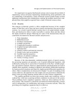
conditions that eliminate the coupling. For instance, for modeling a wall losing
energy by convection to air in a room, as shown in Figure 4.20, the actual thermal
coupling between the airow and conduction in the wall may be replaced by a
heat transfer coefcient h at the wall surface. This decouples the solutions for the
two heat transfer regions since the conditions at the boundary
[] []TT k
T
n
k
T
n
wall air
wall
t
t
§
©
¨
¶
¸
·
t
t
§
©
¨
¶
¸
·
aair
(4.34a)
which requires a solution for the ow and heat transfer in air, are replaced by
t
t
§
©
¨
¶
¸
·
k
T
n
hT T
wall
wall air
() (4.34b)
where n is in the direction normal to the surface and T
air
is a specied tempera-
ture. Similarly, the air is modeled separately for heat transfer with a specied
wall temperature. Then, the two regions are modeled as separate entities without
n
h, T
air
T
air
specified
Air flow
Specified temperature
on boundaries
Room
Air flow
Door
Walls
Wall
Solar
flux
Solar flux
FIGURE 4.20 Decoupling a wall and enclosed air for modeling thermal transport in a
room.
250 Design and Optimization of Thermal Systems
linking the two. Similarly, the condenser in a home air-conditioning system may
be modeled using given, xed inow conditions of the refrigerant to decouple it
from the compressor that provides the input to the condenser in the actual system.
Then each component can be subjected to mathematical modeling procedures
and the resulting mathematical equations derived.
Different simplications and idealizations may apply for different com-
ponents, resulting in different types of governing equations. For example, one
component may be modeled as a lumped mass, giving rise to an ODE for the
temperature as a function of time, while another component may be modeled
as a one-dimensional transient problem, governed by Equation (4.27). A single
nonlinear algebraic equation may arise from an energy balance for determining
the temperature at the surface of a body. The continuity, momentum, and energy
equations may be needed for modeling the ow.
The different mathematical models obtained for the various system parts
are based on simplications, approximations, and idealizations that are, in turn,
based on the material, geometry, transport processes, and boundary conditions.
Estimates of the contributions of the various mechanisms play an important part
in the modeling process. However, the mathematical model derived is not unique
and further improvements may be needed, depending on the numerical results
from simulation and on comparisons with experimental data. Therefore, it is
important to maintain the link between mathematical and numerical models and
to be prepared to improve both as the need arises. It is generally best to start with
the simplest possible mathematical and numerical models and to improve these
gradually by including effects that may have been neglected earlier.
Numerical Modeling
The governing mathematical equations for each component must be solved to
study its behavior. Numerical algorithms applicable to the different types of equa-
tions that arise are employed to solve these equations. Thus, a numerical model,
which is decoupled from the others, is obtained for each component. The results
from this model indicate the basic characteristics of the component under the
idealized or approximated boundary conditions used. The behavior of the compo-
nent, as some of these conditions or related parameters are varied, may be studied
in order to ensure that the individual model is physically realistic. For instance,
the ow rate of the colder uid in a heat exchanger may be increased, keeping the
other variables xed. It is expected that the temperature rise of this uid in the
heat exchanger will decrease because a larger amount of uid is to be heated.
The results from the numerical model must show this trend if the model is physi-
cally valid. Grid renement is also done to ensure the accuracy of the results.
Some simple analytical results, if available, may also be employed to check the
accuracy of the numerical results obtained. Particularly simple cases may be con-
sidered to obtain analytical solutions and thus provide a method of validating the
individual numerical models.
Numerical Modeling and Simulation 251
4.3.2 MERGING OF DIFFERENT MODELS
Once all the individual numerical models for the various components or parts
of the given thermal system have been obtained and tested on the basis of physi-
cal reasoning and analytical results, these must be merged to obtain the model
for the overall system. Such a merging of the models requires bringing back the
coupling between the different parts that had been neglected in the development
of individual models. For instance, if two parts A and B of the system exchange
energy by radiation, their temperatures T
A
and T
B
are coupled through a boundary
condition of the form
Q
AT T
AA B
AB
A
A
A
B
S
EE
44
11
1
(4.35)
where Q is the radiative energy lost by A and gained by B, E
A
and E
B
are the emis-
sivities, and Sis the Stefan-Boltzmann constant. This equation applies for A
completely surrounded by B, with no radiation from A falling directly on itself.
For developing the numerical model for, say, part A, this radiative heat transfer
may be idealized as a constant heat ux q at the surface of A or as a constant
temperature environment in radiation exchange with the surface. Thus, the tem-
perature of part B is eliminated from the model for part A, which may then
be modeled separately. Similarly, such approximations with constant or known
parameters in the boundary conditions may be used for modeling part B. In the
process of merging the two models, these approximations must be replaced by
the actual boundary condition, Equation (4.35), which couples the temperatures
of the two parts.
Similarly, the approximation made in Equation (4.34b) is removed by replac-
ing the convective condition by the correct boundary conditions given by Equation
(4.34a). This couples the transport in the wall with that in the air. For the air-
conditioning system considered earlier, the temperature and pressure at the inlet
of the condenser are set equal to the corresponding values at the exit of the com-
pressor to link these two parts of the system. Proceeding in this way, other parts
are also coupled through the boundary and inow/outow conditions.
This approach of modeling individual parts and then coupling them may
appear to be an unnecessarily complicated way of deriving the numerical model
for the system. Indeed, for relatively simple systems consisting of a small number
of parts, it is often more convenient and efcient to develop the numerical model
for the system without considering individual parts separately. However, if the
system has a large number of parts, it is preferable to develop individual numerical
models and to test and validate them separately before merging them to obtain the
model for the system. This allows a complicated problem to be broken down into
simpler ones that may be individually treated and tested before nal assembly.
This approach is used extensively in industry to model complex systems. A direct
modeling of the entire system has little chance of success because many coupled
252 Design and Optimization of Thermal Systems
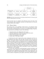
equations are involved. Figure 4.21 shows a schematic of the process described
here for a general thermal system.
4.3.3 ACCURACY AND VALIDATION
We discussed the validation of the mathematical model and the numerical scheme
earlier. Numerical models for individual parts of the system are similarly tested
and validated before merging them to yield the overall numerical model of the
thermal system under consideration. The validation of this complete model,
therefore, is based largely on the testing and validation employed at various steps
along the process. The main considerations that form the basis for validation of
the numerical model of the entire system are, as before,
1. Results should be independent of arbitrary numerical parameters
2. Physical behavior
3. Comparison with analytical and experimental results
4. Comparisons with prototype results
The arbitrary numerical parameters refer to the grid, time step, and other
quantities chosen to obtain a numerical solution. It is important to ensure that
the results from the model are essentially independent of these parameters, as was
done earlier for the numerical solution of individual equations and components.
The physical behavior now refers to the thermal system, so that the results from
the model are considered in terms of the expected physical trends to ascertain
that the model does indeed yield physically realistic characteristics. The numeri-
cal model is subjected to a range of operating conditions and the results obtained
examined for physical consistency.
Numerical
model of system
Physical
system
2
2
2
1
1
13
3
3
Numerical
models
Mathematical
models
Components
FIGURE 4.21 Schematic of the general approach of developing an overall model for a
thermal system.
Numerical Modeling and Simulation 253
Analytical and experimental results are rarely available for validation. How-
ever, as discussed earlier, analytical results may be obtained for a few highly
idealized situations. Similarly, experimental data may be obtained or may be
available for a few simple geometries and conditions. Such analytical results and
experimental data are used for validating mathematical and numerical models
for individual parts of the system. For the overall system, experimental data may
be available from existing systems. For instance, existing cooling and heating
systems may be numerically modeled in order to compare the results against data
available on these systems. Before going into production, a prototype may be
developed to test the model and the design. This provides the best information for
the quantitative validation of the model and a check on the accuracy of the results
obtained from the model.
4.4 SYSTEM SIMULATION
System simulation refers to the process of obtaining quantitative information on the
behavior and characteristics of the real system by analyzing, studying, or examin-
ing a model of the system. The model may be a physical, scaled-down version of the
given system, derived on the basis of the similarity principles outlined in Chapter 3.
Such a model may be subjected to a variety of operating and environmental condi-
tions and the performance of the system determined in terms of variables such as
pressure, ow rate, temperature, energy input/output, and mass transfer rate that are
of particular interest in thermal systems. The results from such a simulation may
be expressed in terms of correlating equations derived by curve-tting techniques.
Physical modeling and testing of full-size components such as compressors, pumps,
and heat exchangers are often used to derive the performance characteristics of
these components. This approach is rarely used for the entire system because of the
cost and effort involved in fabrication and experimentation.
Sometimes the given physical system may be simulated by investigating
another system that is governed by the same equations and that may be easier
to fabricate or assemble. Such a model, called an analog model in the preceding
chapter, also has a limited range of applicability, and, therefore, this simulation is
not often used in the design of thermal systems. Electrical circuits used to simulate
uid-ow systems, consisting of pipes, ttings, valves, and pumps, and conduction
heat transfer through a multi-layered wall are examples of analog simulation.
In the remaining portion of this chapter, we will consider only system simu-
lation based on mathematical and numerical modeling. Therefore, the govern-
ing equations obtained from the mathematical model are solved by analytical
or numerical methods to yield the system behavior under a variety of operat-
ing conditions as well as for different design variables, in order to provide the
quantitative inputs needed for design and optimization. Mathematical solutions
are obtained in only a few, often highly idealized, circumstances, and numerical
modeling is generally needed to obtain the desired results for practical problems.
Performance characteristics of components, as obtained from separate physical
modeling and tests, as well as material properties, form part of the overall model
254 Design and Optimization of Thermal Systems
and are assumed to be known. These may be available in the form of data or
as correlating equations. The governing equations may be algebraic equations,
ordinary or partial differential equations, integral equations, or a combination
of these. Therefore, a numerical model is developed to solve the resulting simul-
taneous equations, many of which are typically nonlinear for thermal systems.
Simulation of the system is carried out by means of this model.
4.4.1 IMPORTANCE OF SIMULATION
System simulation is one of the most important elements in the design and opti-
mization of thermal systems. Since experimentation on a prototype of the actual
thermal system is generally very expensive and time consuming, we have to
depend on simulation based on a model of the given system to obtain the desired
information on the system behavior under different conditions. A one-to-one cor-
respondence is established between the model and the physical system by valida-
tion of the model, as discussed earlier. Then the results obtained from a simulation
of the model are indicative of the behavior of the actual system.
There are several reasons for simulating the system through its mathematical
and numerical model. Simulation can be used to
1. Evaluate different designs for selection of an acceptable design
2. Study system behavior under off-design conditions
3. Determine safety limits for the system
4. Determine effects of different design variables for optimization
5. Improve or modify existing systems
6. Investigate sensitivity of the design to different variables
Evaluation of Design
Evaluation of different designs is an extremely important use of simulation
because several designs are typically generated for a given application. If each
of these were to be fabricated and tested for acceptability, the cost would be pro-
hibitive. System simulation is employed effectively to investigate each design and
to determine if the given requirements and constraints are satised, thus yield-
ing an acceptable or workable design. For instance, several different designs,
employing different geometry, materials, and dimensions, may be developed for
a heat exchanger application involving given uids and given requirements on the
temperatures or the heat transfer rates. Instead of fabricating each of these heat
exchanger designs, mathematical and numerical modeling may be employed to
obtain a satisfactory and accurate model. This model is then used for simulating
the actual system in order to obtain the desired outputs in terms of heat transfer
rates and temperatures. Operating conditions for which the system is designed
are considered rst to determine if the design meets the given requirements and
constraints. These conditions are often termed design conditions because they
form the basis for the design. Even if only one design has been developed for a
given application, it must be evaluated to ensure that it is acceptable.
Numerical Modeling and Simulation 255
Off-Design Performance and Safety Limits
Predicting the behavior of the system under off-design conditions, i.e., values
beyond those used for the design, is another important use of system simulation.
Such a study provides valuable information on the operation of the system and
how it would perform if the conditions under which it operates were to be altered,
as under overload or fractional-load circumstances. Systems seldom operate at the
design conditions and it is important to determine the range of operating condi-
tions over which they would deliver acceptable results. The deviation from design
conditions may occur due to many reasons, such as variations in energy input,
differences in raw materials fed into the system, changes in the characteristics
of the components with time, changes in environmental conditions, and shifts in
energy load on the system. The results obtained from simulation under off-design
conditions would indicate the versatility and robustness of the system. It is obvi-
ously desirable to have a wide range of off-design conditions for which the system
performance is satisfactory. A narrow range of acceptability is generally not suit-
able for consumer products because large variations in the operating conditions
are often expected to arise. For instance, a residential hot-water system designed
for a particular demand and given inlet temperature must be able to perform satis-
factorily if either of these were to vary substantially. In manufacturing processes,
it is common to encounter variations in the shape, dimensions, and material prop-
erties of the items undergoing thermal processing.
These outputs also indicate the safety limits of the system. It is important to
determine the maximum thermal load an air conditioner can take, the maximum
power input to a furnace that can be given, and so on, without damage to the
system or the user. Safety features can then be built into the system, such as man-
datory shutdown of the system if the safety levels are exceeded or warning lights
to indicate possible damage to the system. We are all familiar with such features
in cars, lawn mowers, and other systems in daily use. Some of these aspects were
also considered earlier in Section 2.3.6.
Optimization
System simulation plays an important role in optimization of the system. As will
be seen in later chapters, the outputs from the system must be obtained for a range
of design variables in order to select the optimum design. The optimization of the
system may involve minimization of parameters such as cost per item, weight, and
energy consumption per unit output or maximization of quantities such as out-
put, return on investment, and rate of energy removal. Whatever the criterion for
optimization, it is essential to change the variables over the design domain, deter-
mined by physical limitations and constraints, and to study the system behavior.
Then, using the various techniques for optimization presented later, the optimal
design is determined. The results obtained from simulation may sometimes be
curve tted to yield algebraic equations, which greatly facilitate the optimiza-
tion process. For instance, if the cooling system for an electronic equipment has
been designed using a fan, different locations, ow rates, and dimensions of the
256 Design and Optimization of Thermal Systems
fan may be considered to derive algebraic equations to represent the dependence
of the heat removal rate on these variables. Then, an optimal conguration that
delivers the most effective cooling per unit cost may be obtained easily.
Modifications in Existing Systems
The use of simulation for correcting a problem in an existing system or for modi-
fying the system for improving its performance is also an important application.
Rather than changing a particular component in order to correct the problem
or improve the system, simulation is rst used to determine the effect of such a
change. Since the simulation closely represents the actual physical system, the
usefulness of the proposed change can be determined without actually carrying
out the change. For instance, if a ow system is unable to deliver the expected
ow rates, the problem may lie with various sections of the piping, pipe ttings,
valves, or pumps. Instead of proceeding to change a given valve or pump, simula-
tion may be used to determine if indeed the problem is caused by a particular item
and if an improved version of the item will be worthwhile. It may be shown by the
simulation that the lack of ow at a given point is due to some other cause, such as
blockage in a particular section of the piping. Clearly, considerable savings may
be obtained by using simulation in this manner.
Sensitivity
A question that arises frequently in design is the effect of a given variable or
component on the system performance. For instance, if the dimensions of the
channels or of the collectors in a solar collection system were varied, what would
be the overall effect on the system? Similarly, if the capacity of the fan or blower
in a cooling system were varied, how would it affect the heat removal rate? Such
questions relate to the sensitivity of the system performance to the design vari-
ables and are important from a practical viewpoint. A substantial reduction in the
cost of the system may be obtained by slight changes in the design in order to use
standard items available in the market. Pipes and tubings are usually available at
xed dimensions and if these could be employed in the system, rather than the
exact custom-made dimensions, substantial savings may result. Similarly, uid
ow components such as blowers, pumps, and fans are often cheaply and eas-
ily available for given specications. At different values, these may have to be
fabricated individually, raising the price substantially. System simulation is used
to determine the sensitivity of the system performance to such variables and to
decide if slight alterations can be made in the interest of reducing the cost without
signicant sacrice in system characteristics.
4.4.2 DIFFERENT CLASSES
Several types of simulation are used for thermal systems. We have already men-
tioned analog and physical simulations, which are based on the corresponding
form of modeling, as discussed in Chapter 3. In this chapter, we have focused on
Numerical Modeling and Simulation 257
numerical modeling and numerical simulation, which are based on the mathemat-
ical modeling of the thermal system. Three main classes of this form of system
simulation are discussed here.
DynamicorSteadyState
The simulation of a system may be classied as dynamic or steady state. The
former refers to the circumstances where changes in the operating conditions and
relevant system variables occur with respect to time. Many thermal systems are
time-dependent in nature and a dynamic simulation is essential. This is particu-
larly true for the start-up and shutdown of the system. Also, in most manufactur-
ing processes the temperature and other attributes of the material undergoing
thermal processing vary with time, as shown in Figure 2.1. The system itself may
vary with time over the duration of interest due to energy input as in welding, gas
cutting, heat treatment, and metal forming. In processes such as crystal growing,
ingot casting, and annealing, the system varies with time along with the tempera-
ture of the material being processed. Dynamic simulation is also needed to study
the response of the system to changes in the operating conditions such as a sharp
increase in the heat load on a food freezing plant. The results obtained from a
dynamic simulation are also useful in the design and study of the control scheme
for a satisfactory operation of the system.
Steady-state simulation refers to situations where changes with respect to
time are negligible or do not occur. Since the dependence of the variables on time
is eliminated, a steady-state simulation is much simpler than the corresponding
dynamic simulation. In addition, the steady-state approximation can be made in a
large number of practical cases, making steady-state simulation of greater interest
and importance in thermal systems. Except for times close to start-up and shut-
down, many systems behave as if they are under steady-state conditions. Thus,
a blast furnace may be treated as essentially steady over much of its operation.
A typical system that is transient at the beginning and end of its operation and
steady over the rest is shown in Figure 4.22. In addition, the system itself may be
approximated as steady even though the temperature of the material undergoing
Time
Shutdown
Steady
Start-up
Temperature
FIGURE 4.22 Temperature variation in a typical thermal system that is steady over most
of the duration of operation and is time-dependent only near start-up and shutdown.
258 Design and Optimization of Thermal Systems
thermal processing varies with time. An example of this is a circuit board being
baked. The baking oven may be approximated as being unchanged and operating
under steady-state conditions while the board undergoes a relatively large tem-
perature change as it moves through the oven.
Continuous or Discrete
In many systems such as refrigeration and air-conditioning systems, power plants,
internal combustion engines, and gas turbines, the ow of the uid may be taken
as continuous, with no nite gaps in the uid stream. Thus, a continuum of the
material or the uid is assumed, with the conservation laws derived based on a
continuum approximation. This implies the use of continuity, momentum, and
energy equations from uid mechanics and heat transfer for transport processes
in a continuum. Particles, if present in the ow, are not treated separately but as
part of the average properties of the uid. Most thermodynamic systems can be
simulated as continuous because energy and uid ow are generally continuous
[see Figure 4.23(a)].
On the other hand, if discrete pieces, such as ball bearings, fasteners, and
gears, undergoing thermal processing, are considered, the simulation focuses on
a nite number of such items. In the manufacture of television sets, individual
glass screens are heat treated as they pass through a furnace on a conveyor belt,
as sketched in Figure 4.23(b). In such cases, the mass, momentum, and energy
(b)
(a)
q
Reflector
Discrete items
Heater panels
Conveyor belt
U
Component 2
Component 1
Flow
q
FIGURE 4.23 (a) Continuous and (b) discrete simulation.
Numerical Modeling and Simulation 259
balances of each item are considered separately to determine, for instance, the
temperature as a function of time. An aggregate or an average may be obtained at
the end to quantify the process, if desired. An example of this class of simulation
is provided by the modeling of the movement of a plastic piece as it goes from the
hopper to the die in an extruder to determine the time taken (generally known as
residence time). An average residence time may be dened by considering several
such pieces.
Deterministic or Stochastic
In most of the examples of thermal processes and systems considered thus far,
the variables in the problem are assumed to be specied with precision. Such
processes are known as deterministic. However, there are several cases where
the input conditions are not known precisely and a probability distribution may
be given instead, with a dominant frequency, an average, and an amplitude of
variation. The conditions may also be completely random with an equal probabil-
ity of attaining any value over a particular range. When dealing with consumer
demands for power, hot water, supplies, etc., probabilistic descriptions are often
employed and the corresponding simulation, known as stochastic, is carried out to
determine the appropriate design variables. A useful simulation method, known
as the Monte Carlo method, uses the randomness of the process along with given
probability distributions to simulate the system to determine the resulting average
output, transport rate, time taken, and other characteristics. Employing random
numbers generated on the computer, events are selected from the given distribu-
tion to simulate the randomness in selection. The various steps in the overall pro-
cess are followed to obtain the result for a given starting point. An aggregate of
several such simulations yields the expected average behavior of the system. This
approach is often used in manufacturing systems to account for statistical varia-
tions at different stages of the process (Dieter, 2000; Ertas and Jones, 1996).
4.4.3 FLOW OF INFORMATION
A useful concept in the simulation of thermal systems is that of information ow
between the different parts, components, or subsystems that make up the system.
The ow of information from one part to another is largely in terms of quantities
that are of particular interest to thermal systems, such as temperature, velocity,
ow rate, and pressure, and indicates the nature of coupling between the two.
The input to a given item undergoing thermal processing or to a continuous ow
may be provided by the system parts and, similarly, the output from this item
or ow may be fed to these parts. This involves the transport of mass, momen-
tum, and energy as a discrete item or a continuous ow goes through the system.
Clearly, different types of information ow arrangements may arise, depending
on the thermal system. Such arrangements are often shown as information-ow
diagrams in which the various parts of the system are linked through inputs and
outputs. The strategy for simulating the system is often guided by the nature and
characteristics of information ow between the different parts of the system.
260 Design and Optimization of Thermal Systems
Block Representation
Each component may itself be represented as a block with characteristic or inputs
and outputs. For instance, a compressor may be represented by a block with the
inlet pressure p
1
and the mass ow rate
m as inputs and the outlet pressure p
2
as
the output. The efciency and discharge rate may also be taken as outputs. The
equation that expresses the relationship between these variables may be writ-
ten within the block to indicate the characteristics of the component. Again, this
equation may be an algebraic, differential, or integral equation, or a combination
of these. For steady-state problems, assuming uniformity in each component, the
characteristic equation linking the inputs and outputs will be an algebraic equa-
tion. ODEs arise for transient cases, if uniformity or lumping is still assumed
within each component or part. PDEs arise for general, distributed, or nonuni-
form cases. Similarly, a heat exchanger may be represented by a block, with
ow rates
m
1
and
m
2
of the two streams and inlet temperatures T
1,i
and T
2,i
as the
inputs. Then, the outlet temperature T
2,0
of one stream may be taken as the output,
with
fm m T T T
ii
(, , , , )
,,,
121 2 20
0
representing the relationship between the inputs
and the outputs. Figure 4.24 shows typical blocks that may be used to represent a
few components of interest to thermal systems. Obviously, other combinations of
inputs and outputs are possible and may be employed depending on the specic
application. The use of such blocks to represent the system components facilitates
the representation of the overall system in terms of the information ow between
different parts.
Information Flow
A diagram showing the ow of information for a system is constructed using blocks
for the various parts of the system. Let us consider the relatively complex problem
of a plastic screw extrusion system, as shown in Figure 1.10(b). The plastic mate-
rial is conveyed, heated, melted, and forced through the die due to the rise in pres-
sure $p and temperature $T in the extruder. The transport processes are governed
by nonlinear PDEs, further complicated by material property variations, complex
Pump
Compressor
m
m
condensed
Condenser
Heat exchanger
p
2
p
1
m
1
m
1
, m
2
m
1
p
1
T
1,o
T
1,i
, T
2,i
T
1,i
T
2,o
p
2
.
.
.
.
.
.
FIGURE 4.24 Block representations of a few common components used in thermal
systems.
Numerical Modeling and Simulation 261
geometry, and the phase change. However, the extruder may be numerically simu-
lated to study the dependence of temperature and pressure on the inputs such as
mass ow rate
m, speed N in revolutions per minute, and barrel temperature T
b
.
These simulation results may be curve tted to obtain an algebraic equation. If the
hopper, extruder, and die are taken as the three parts of the system, Figure 4.25
shows the information-ow diagram for this circumstance with the following equa-
tions expressing the relationships between the inputs and outputs for these three
parts, respectively:
fDm
fmNT p T
fpT
b
1
0(,)
2
3
(, , , , ) 0
(, ,
$$
$$ )0
m
(4.36)
Here, the extruder and the die are taken as xed, so that only the operating condi-
tions are varied. D is the diameter of the opening of the hopper and, thus, repre-
sents its geometry.
The pressures at the entrance to the hopper and at the exit of the die are taken
as atmospheric. Here, f
1
and f
2
represent the characteristics of the hopper and the
die, respectively. The mass ow rate into the die must equal that emerging from
the extruder from mass conservation considerations for steady-state operation. The
motor that provides the torque and the heater that supplies the heat input to the
barrel are additional parts that may be included, as shown by dotted lines in the
gure. The extruder itself may be considered to consist of different zones that are
modeled separately, such as the solid conveying, melting, and metering sections.
Again, these are coupled through the ow rate
m and the temperature and pressure
continuity. For further details on this system, specialized books, such as those by
Tadmor and Gogos (1979) and Rauwendaal (1986), may be consulted.
Heater
f
4
(q, T
b
) = 0
f
2
(m, N, T
b
,Δp,ΔT) = 0f
1
(D, m) = 0
f
5
(S, N) = 0
D
Hopper
m
N
f
3
(Δp,ΔT, m) = 0
Die
Screw
extruder
Torque (S)
Motor
mΔp,ΔT
T
b
q
.
.
.
.
.
FIGURE 4.25 Information-ow diagram for a screw extrusion system.
262 Design and Optimization of Thermal Systems
The information-ow diagram for a vapor-compression cooling system, shown
in Figure 1.8(a), may be similarly drawn. The characteristics of the compressor,
condenser, throttling valve, and evaporator can be expressed by the equations
f
1
(p
1
, h
1
, p
2
, h
2
) 0
f
2
(p
2
, h
2
, h
3
) 0
f
3
(p
1
, p
2
) 0
(4.37)
f
4
(p
1
, h
3
, h
1
) 0
where the different states are shown on a p-h plot of the thermodynamic cycle in
Figure 4.26(a). The information-ow diagram is shown in Figure 4.26(b). Con-
servation of enthalpy in the throttling process, h
3
h
4
, is employed and the char-
acteristic equations are derived for a given uid such as a chlorouorocarbon
(CFC). The inlet into each part corresponds to the exit from the preceding one in
this closed cycle.
The information-ow diagram for the electric furnace shown in Figure 4.27(a)
is more involved than the preceding two cases because energy transfer occurs
between different parts of the system simultaneously. Thus, the heater exchanges
thermal energy with the walls, gases, and material. Similarly, the material under-
going heat treatment is in energy exchange with the heater, walls, and gases.
Example 3.6 derived the mathematical model for this system. Figure 4.27(b)
(b)
(a)
Enthalpy
1
23
4
Pressure
h
1
p
1
h
3
h
2
p
2
h
1
p
1
Evaporator
f
4
( p
1
, h
3
, h
1
)
=0
rottling valve
f
3
(p
2
, p
1
) = 0
Condenser
f
2
(p
2
, h
2
, h
3
)
=0
Compressor
f
1
(p
1
, h
1
, p
2
, h
2
)
=0
FIGURE 4.26 A vapor-compression cooling system. (a) Thermodynamic cycle; (b) infor-
mation-ow diagram.
Numerical Modeling and Simulation 263
shows a sketch of the information-ow diagram for this circumstance, strongly
coupling all the parts of the system. The ow of information between any two
parts is due to energy transfer that involves combinations of the three modes:
radiation, convection, and conduction. The governing equations are ordinary
and partial differential equations for the transient problem, as modeled in
Example 3.6.
In each of the three cases just outlined, different information-ow diagrams
are obtainable by choosing different starting points and different inputs/outputs.
The diagrams indicate the link between different parts of the system and thus sug-
gest ways of approaching the simulation. In the rst two examples of the extruder
and the air-conditioning system, the output from one component feeds into the
next as an input. The overall arrangement is sequential because one part depends
only on the preceding one. However, in the furnace, a part is simultaneously cou-
pled with several others through the energy exchange mechanisms. Therefore, in
the former circumstances a sequential calculation procedure is appropriate for the
simulation, whereas a simultaneous solution procedure is essential for the latter.
Material
Wall
Gases
Insulation
Heat loss
Ambient
Heater
(b)
(a)
Ambient
Insulation
WallMaterial
Heater
Q
Gases
FIGURE 4.27 (a) An electric furnace; (b) information-ow diagram showing the cou-
pling between different parts of the system.
264 Design and Optimization of Thermal Systems
4.5 METHODS FOR NUMERICAL SIMULATION
The method appropriate for simulating a given thermal system is strongly depen-
dent on the nature of the system and, thus, on the characteristics of the governing
equations. These are best specied in terms of the mathematical model. Let us
consider a few important types of systems and their corresponding simulations.
4.5.1 STEADY LUMPED SYSTEMS
This is the simplest circumstance in the modeling and simulation of thermal sys-
tems. If the system can be modeled as steady, the dependence of the variables
on time is eliminated. In addition, if uniform conditions are assumed to exist in
the various components or parts of the system, implying that they are treated as
lumped, spatial distributions of variables such as temperature and pressure do not
arise. Then the governing equations are simply algebraic equations, which may be
linear or nonlinear. The equations are coupled to each other through the unknowns,
which are the inputs and outputs to the different blocks in an information-
ow diagram, as seen earlier. The external inputs to the overall system are given
or may be varied in the simulation and the overall outputs from the system repre-
sent the information desired from the simulation.
Most thermodynamic systems, such as power plants, air conditioners, internal
combustion engines, gas turbines, compressors, pumps, etc., can usually be mod-
eled as steady and lumped without much sacrice in the accuracy of the simula-
tion (Howell and Buckius, 1992; Moran and Shapiro, 2000). Similarly, uid ow
systems, such as network pipes, can often be treated as steady and lumped.
The governing algebraic equations in steady lumped systems may be written as
f
1
(x
1
, x
2
, x
3
, z, x
n
) 0
f
2
(x
1
, x
2
, x
3
, z, x
n
) 0
f
3
(x
1
, x
2
, x
3
, z, x
n
) 0
(4.38)
f
n
(x
1
, x
2
, x
3
, z, x
n
) 0
where the x’s represent the unknowns and the equations may be linear or non-
linear. If all the equations are linear, the system of equations may be solved by
direct or iterative methods, using the former approach for relatively small sets of
equations and for tridiagonal systems, and the latter for large sets, as discussed
earlier. However, several equations in the set of algebraic equations governing
typical thermal systems are usually nonlinear, making the solution much more
involved than that for linear equations.
Successive Substitution Method
The two main approaches used for simulating thermal systems governed by non-
linear equations are based on the successive substitution and Newton-Raphson
Numerical Modeling and Simulation 265
methods, which were discussed in Section 4.2.2 for a single nonlinear algebraic
equation and for a set of nonlinear equations. Let us rst consider the succes-
sive substitution method. In this case, for a single equation, the iterative solution
obtained by solving the equation is substituted back into the equation and the
iterations continued until convergence is achieved, as indicated by an acceptable
small variation in the solution from one iteration to the next. For a system of equa-
tions, each equation is solved for an unknown using known values from previ-
ous iterative calculations. This solution is then substituted into the next equation,
which is solved to obtain another unknown. This is again substituted into the next
equation, in succession, and the process is continued until the solution obtained
does not vary signicantly from one iteration to the next. A scheme such as the
modied Gauss-Seidel method given in Equation (4.19) may be used effectively
to simulate the system.
The numerical algorithm is quite simple for this method. Relaxation may also
be used to improve the convergence. SUR is particularly useful in obtaining con-
vergence in nonlinear equations. Thus, if the relaxation factor W is in the range
0 W 1, SUR is applied as
x Gxx xx
i
l
i
ll
i
l
i
l()
() () ()
(
,,,,
1
1
1
2
1
1
1
W
))() ()
,, ( )
xx
in
n
l
i
l
§
©
¶
¸
1 W
for 1, 2, ,
(4.39)
The successive substitution method is particularly well suited for sequential
information-ow diagrams, such as those in Figure 4.25 and Figure 4.26. The
equations corresponding to the different parts of the system are solved in succes-
sion, using the inputs from the preceding part or equation, until convergence of
the iteration is achieved to a chosen convergence criterion, as given by Equation
(4.7). The method can be applied to large systems involving large sets of nonlin-
ear algebraic equations. Computer storage requirements are small and computer
programming is fairly simple. As a result, this approach is extensively used in
industry for simulating steady-state thermal systems in mechanical and chemical
engineering processes.
The main problem with the successive substitution method is difculty in
convergence of the iterative process. For sequential information-ow diagrams,
convergence is much more easily obtained than for simultaneous information-
ow cases, sketched in Figure 4.27, since the numerical simulation follows the
physical characteristics of the system in the former circumstance. Convergence is
strongly dependent on the starting point and on the arrangement of the equations
for solution. As seen earlier for linear systems, diagonal dominance is needed to
assure convergence. Therefore, in linear systems the equations are arranged in
order to place the dominant coefcient at the diagonal of the coefcient matrix,
implying that each equation is solved for the unknown with the largest coef-
cient. Though the corresponding convergence characteristics are not available for
nonlinear equations, a change in the arrangement of the equations can affect the
convergence substantially. Generally, information blocks should be positioned so
266 Design and Optimization of Thermal Systems
that the effect on the output is small for large changes in the input. The equations
may be rewritten to achieve this. Stoecker (1989) gives a few examples in which
the sequence of the equations and thus of the unknowns being solved can be
changed to obtain convergence. Similarly, the starting values should be picked
based on the physical background of the given system so that these are realistic
and as close as possible to the nal solution. Again, SUR may be used for cases
where convergence is a problem. A few examples are included later in this chapter
to illustrate these strategies.
Newton-Raphson Method
The second approach for solving a set of nonlinear algebraic equations is the
Newton-Raphson method discussed in Section 4.2.2 for a single nonlinear equa-
tion and then extended to a set of nonlinear algebraic equations. This method is
appropriate for an information-ow diagram in which a strong interdependence
arises between the different parts of the system, such as that shown in Figure 4.27.
The convergence characteristics are generally better than those for the successive
substitution, or modied Gauss-Seidel, method. However, the method is much
more complicated since the matrix of derivatives, given in Equation (4.17) and
generally known as the Jacobian, has to be calculated at each iterative step.
Since the computed variation of each of the functions f
i
with the unknowns x
i
is employed in determining the changes in x
i
for the next iteration, the iterative
scheme is much better behaved than the successive substitution method, which
does not use any such quantitative measure of the change in f
i
with x
i
. However,
the derivatives may not be easily obtainable by analysis and numerical differ-
entiation may be necessary, further complicating the procedure. Generally, the
Newton-Raphson method is useful for relatively small sets of nonlinear equations
and for cases where the derivatives can be obtained easily. However, different
approaches have been developed in which the derivatives are computed numeri-
cally by efcient algorithms as the iterative scheme proceeds. For instance, the
partial derivative ∂f
i
/∂x
j
may be computed as
t
t
f
x
fxx x x x fxx x
i
j
ijjni
(,,, ,,) (,,,
12 12
$
jjn
j
x
x
,,)
$
(4.40)
where $x
j
is a chosen increment in x
j
. Thus, all the partial derivatives needed for
Equation (4.17) are computed at each iteration and the next approximation to the
solution obtained, carrying out this procedure until convergence to the chosen
convergence criterion is achieved.
The Newton-Raphson approach links all the parts of the system simultane-
ously through the derivatives. Thus, changes in one component will affect all oth-
ers at the same time and the effect is dependent on the corresponding derivatives.
Therefore, the approach follows the physical behavior of systems where all the
parts are strongly linked with each other. Several thermal systems, such as those
Numerical Modeling and Simulation 267
in manufacturing and cooling of electronic equipment, have strong, simultane-
ous coupling between the different parts, making it desirable to use the Newton-
Raphson method. However, if the systems have a large number of parts, leading
to a large number of algebraic equations, it may be more advantageous to use the
successive substitution approach, employing under-relaxation for better conver-
gence. The examples that follow illustrate these methods of simulation.
Example 4.6
In the ammonia production system sketched in Figure 4.28, a mixture of 90 moles/s
of nitrogen, 270 moles/s of hydrogen, and 0.9 moles/s of argon enters the plant and is
combined with the residual mixture crossing a bleed valve. Argon is an impurity and
adversely affects the reaction (Stoecker, 1989; Parker, 1993). In the chemical reactor,
a fraction of the entering mixture combines to form ammonia, which is removed by
condensation. The bleed valve removes 23.5 moles/s of the mixture to avoid build-up
of argon. The fraction of the mixture that reacts to give ammonia in the reactor is
0.57 exp(–0.0155 F
1
), where F
1
is the amount of argon entering the reactor in moles
per second. Solve the resulting set of algebraic equations by the successive substitu-
tion approach to obtain the ow rates and the amount of ammonia produced.
Solution
The governing system of algebraic equations may be derived based on mass conser-
vation. If F
1
and F
2
are the ow rates of argon and nitrogen, respectively, in moles
per second entering the reactor, the ow rate of hydrogen is 3F
2
moles/s from the
chemical reaction, which yields ammonia. Then, we obtain
F
B
F
BP
1
2
09
1
90
1
.
()
()
Bleed
Reaction
chamber
Liquid
ammonia
Condenser
Nitrogen,
hydrogen, and
argon
FIGURE 4.28 The ammonia production system considered in Example 4.6.
268 Design and Optimization of Thermal Systems
where
PF
B
FP F
1 0.57 exp( 0.0155 )
1
1
23 5
4
21
.
Here, P represents the fraction of unconverted mixture of nitrogen and hydrogen
and B represents the fraction of mixture that goes past the bleed valve. The chemi-
cal reaction for producing ammonia is
N
2
3H
2
2NH
3
Therefore, the amount of ammonia produced D is given by
D 2F
2
[0.57 exp(0.0155 F
1
)]
The governing system of four nonlinear algebraic equations may be rewritten
to solve for the four unknowns F
1
, F
2
, P, and B in sequence, terminating the itera-
tion when values do not change signicantly from one iteration to the next. The
equations and unknowns can be arranged in several ways to apply the successive
substitution method. Many of these do not converge and solving the equations in
a different order, as well as using different starting values, is tried. The computer
programming is very simple, but the scheme diverges in many cases.
The method is found to converge if a starting value of B is taken and the four
equations are solved in the following sequence:
F
B
PF
F
1
2
09
1
90
1
.
()
(
1 0.57 exp( 0.0155 )
1
BBP
B
FP F
)
.
1
23 5
4
21
The convergence criterion may be applied to B or to the total ow rate F entering
the reactor, where F F
1
4F
2
.
Applying the convergence criterion to F with the convergence parameter E taken
as 10
–4
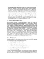
, the numerical results obtained are shown in Figure 4.29. The argon ow rate
and the total ow rate entering the reactor are computed, along with the amount of
ammonia produced, for each iteration. The convergence is found to be slow because
of the rst-order convergence of the method. It is ensured that the results are essen-
tially independent of the value of E chosen by varying E. The numerical method
is extremely simple and is frequently applied to solve sets of nonlinear equations
that arise in such thermal systems. The main problem is convergence, and differ-
ent starting values as well as different formulations and solution sequences of the
Numerical Modeling and Simulation 269
algebraic equations may be tried to obtain convergence. SUR may also be used
for improving the convergence characteristics. The method is popular because no
derivatives are needed, as is the case for the Newton-Raphson method.
Example 4.7
In a thermal system, the volume ow rate R of a uid through a duct due to a fan is
given in terms of the pressure difference P, which drives the ow as
R 15 75 r 10
6
r P
2
with
P 80 10.5R
5/3
where R is in m
3
/s and P is in N/m
2
. The rst equation represents the characteristics
of the fan and the other that of the duct. Simulate this system by the successive
substitution and Newton-Raphson methods to obtain the ow rate and pressure
difference.
Solution
From the physical nature of the problem, we know that both P and R must be real
and positive. Figure 4.30 shows the characteristics of the fan-duct system in terms
of the ow rate R versus pressure difference P graphs. As the pressure difference
168.69990
168.69990
168.69990
168.69990
168.69990
168.69990
168.69980
168.69970
168.69950
168.69900
168.69830
168.69680
168.69410
168.68890
168.67910
168.66060
168.62510
168.55670
168.42190
168.14510
167.52770
165.87840
158.95630
105.65780NH3:
NH3:
NH3:
NH3:
NH3:
NH3:
NH3:
NH3:
NH3:
NH3:
NH3:
NH3:
NH3:
NH3:
NH3:
NH3:
NH3:
NH3:
NH3:
NH3:
NH3:
NH3:
NH3:
NH3:
FLOW:
FLOW:
FLOW:
FLOW:
FLOW:
FLOW:
FLOW:
FLOW:
FLOW:
FLOW:
FLOW:
FLOW:
FLOW:
FLOW:
FLOW:
FLOW:
F
LOW:
FLOW:
FLOW:
FLOW:
FLOW:
FLOW:
FLOW:
FLOW:
ARGON:
Results
ARGON:
ARGON:
ARGON:
ARGON:
ARGON:
ARGON:
ARGON:
ARGON:
ARGON:
ARGON:
ARGON:
ARGON:
ARGON:
ARGON:
ARGON:
ARGON:
ARGON:
ARGON:
ARGON:
ARGON:
ARGON:
ARGON:
ARGON:
793.41060
793.41060
793.41040
793.40990
793.40890
793.40720
793.40450
793.39960
793.38960
793.37080
793.33560
793.26920
793.14420
792.90770
792.46190
791.62100
790.03320
787.03170
781.34420
770.51630
749.70330
708.79150
621.94090
377.52020
17.46423
17.46423
17.46422
17.46417
17.46411
17.46400
17.46382
17.46347
17.46278
17.46149
17.45906
17.45448
17.44583
17.42950
17.39871
17.34062
17.23091
17.02342
16.62993
15.88013
14.43962
11.64363
6.36528
1.00000
FIGURE 4.29 Numerical results obtained for Example 4.6.
270 Design and Optimization of Thermal Systems
P needed for the ow increases, due to blockage or increased length of duct, the
ow generated by the fan decreases, ultimately becoming zero at P of 447.2 N/m
2
.
The pressure difference P in the duct is smallest at zero ow and increases as the
ow rate increases. In addition, the given equations indicate that P must be greater
than 80 and R must be less than 15, giving ranges for these variables for selecting
the starting values.
The two equations are already given in the form x
i
F
i
(x
1
, x
2
, z, x
i
, z, x
n
),
which is appropriate for the application of the successive substitution, or modi-
ed Gauss-Seidel, method. However, when the equations are employed as given,
with starting values taken for P and R from their appropriate ranges, the scheme
diverges rapidly. As mentioned earlier, if an equation x g(x) is being solved for the
root A by the successive substitution method, the absolute value of the asymptotic
convergence factor g`(A) must be less than 1.0 for convergence. An estimation of
the corresponding values of g` in the given equations indicates that these values are
much greater than 1.0.
Since both P and R are greater than 1.0, a reformulation of the equations may
be carried out to yield
R
P
P
R
§
©
¨
¶
¸
·
r
§
©
¨
¶
¸
·
80
10 5
15
75 10
35
6
1
.
/
/
and
22
so that fractional powers are involved and g` becomes less than 1.0. The successive
substitution scheme, when applied to these equations with starting values in the ranges
R
P
P
P
R
R
Duct
Fan
447.2
15
80
FIGURE 4.30 Characteristic curves, in terms of pressure difference versus ow rate
graphs, for the fan and the duct, respectively system considered in Example 4.7.
Numerical Modeling and Simulation 271
0 R 15 and 447.2 P 80, converges to yield the desired solution. The initial
guesses for P and R are substituted on the right-hand sides of these equations to calcu-
late the new values for R and P. These are resubstituted in the equations to obtain the
values for the next iteration, and so on. The iterative process is terminated if
(R
i1
R
i
)
2
(P
i1
P
i
)
2
aE
where the subscripts indicate the iteration number and E is a chosen small quantity.
The numerical results during the iteration are shown in Figure 4.31 for E 10
–6
and the starting values for P and R taken as 80 and 0, respectively. The scheme
converges to P 332.0353 and R 6.7314, both variables being in their allowable
ranges. The results were not signicantly altered at still smaller values of E.
To apply the Newton-Raphson method, these equations are rewritten in terms
of functions F and G as
FPR
P
R
GPR
R
(, )
.
(, )
/
§
©
¨
¶
¸
·
r
80
10 5
0
15
75 1
35
00
0
6
12
§
©
¨
¶
¸
·
/
P
Initial guesses are taken for P and R, as before, and the values for the next iteration,
i 1, are obtained from the values after the ith iteration as
P
i1
P
i
($P)
i
and R
i1
R
i
($R)
i
P
P
R
R
FIGURE 4.31 Computer output for the solution to the problem considered in Example 4.7
by the successive substitution method.