Designing Capable and Reliable Products Episode 1 Part 10 pps

more so when process shift is taken into account, as shown by the term 
H
. Anticipation
of the shift or drift of the tolerances set on a design is therefore an important factor
when predicting reliability. It can be argued that the dimensional variability estimates
from CA apply to the early part of the product's life-cycle, and may be overconservative
when applied to the useful life of the product. However, variability driven failure occurs
throughout all life-cycle phases as discussed in Chapter 1.
From the above arguments, it can be seen that anticipation of the process capability
levels set on the important design characteristics is an important factor when predict-
ing reliability (Murty and Naikan, 1997). If design tolerances are assigned which have
large dimensional variations, the eect on the reliability predicted must be assessed.
Sensitivity analysis is useful in this respect.
Stress concentration factors and dimensional variability
Geometric discontinuities increase the stress level beyond the nominal stresses
(Shigley and Mischke, 1996). The ratio of this increased stress to the nominal stress
in the component is termed the stress concentration factor, Kt. Due to the nature
of manufacturing processes, geometric dimensions and therefore stress concentra-
tions vary randomly (Haugen, 1980). The stress concentration factor values, however,
are typically based on nominal dimensional values in tables and handbooks. For
example, a comprehensive discussion and source of reference for the various stress
concentration factors (both theoretical and empirical) for various component
con®gurations and loading conditions can be found in Pilkey (1997).
Underestimating the eects of the component tolerances in conditions of high
dimensional variation could be catastrophic. Stress concentration factors based on
nominal dimensions are not sucient, and should, in addition, include estimates
based on the dimensional variation. This is demonstrated by Haugen (1980) for a
notched round bar in tension in Figure 4.20. The plot shows Æ3 con®dence limits
on the stress concentration factor, Kt, as a function of the notch radius, generated
using a Monte Carlo simulation. At low notch radii, the stress concentration factor
predicted could be as much as 10% in error from the results.

The main cause of mechanical failure is by fatigue with up to 90% failures being
attributable. Stress concentrations are primarily responsible for this, as they are
among the most dramatic modi®ers of local stress magnitudes encountered in
design (Haugen, 1980). Stress concentration factors are valid only in dynamic
cases, such as fatigue, or when the material is brittle. In ductile materials subject to
static loading, the eects of stress concentration are of little or no importance.
When the region of stress concentration is small compared to the section resisting
the static load, localized yielding in ductile materials limits the peak stress to the
approximate level of the yield strength. The load is carried without gross plastic
distortion. The stress concentration does no damage (and in fact strain hardening
occurs) and so it can be ignored, and no Kt is applied to the stress function. However,
stress raisers when combined with factors such as low temperatures, impact and
materials with marginal ductility could be very signi®cant with the possibility of
brittle fracture (Juvinall, 1967).
For very low ductility or brittle materials, the full Kt is applied unless information
to the contrary is available, as governed by the sensitivity index of the material, q
s
.
For example, cast irons have internal discontinuities as severe as the stress raiser
Variables in probabilistic design 165
itself, q
s
approaches zero and the full value of Kt is rarely applied under static loading
conditions. The following equation is used (Edwards and McKee, 1991; Green, 1992,
Juvinall, 1967; Shigley and Mischke, 1996):
K
H
 1  q
s
Kt ÿ 14:22

where:
K
H
 actual stress concentration factor for static loading
q
s
 index of sensitivity of the material (for static loading
ÿ
0.15 for hardened
steels, 0.25 for quenched but untempered steel, 0.2 for cast iron;
for impact loading
ÿ
0.4 to 0.6 for ductile materials, 0.5 for cast iron,
1 for brittle materials):
In the probabilistic design calculations, the value of Kt would be determined from the
empirical models related to the nominal part dimensions, including the dimensional
variation estimates from equations 4.19 or 4.20. Norton (1996) models Kt using
power laws for many standard cases. Young (1989) uses fourth order polynomials.
In either case, it is a relatively straightforward task to include Kt in the probabilistic
model by determining the standard deviation through the variance equation.
The distributional parameters for Kt in the form of the Normal distribution can
then be used as a random variable product with the loading stress to determine the
®nal stress acting due to the stress concentration. Equations 4.23 and 4.24 show
Figure 4.20
Values of stress concentration factor, Kt, as a function of radius, r, with Æ3 limits for a
circumferentially notched round bar in tension [d $ N(0.5, 0.00266) inches, 
r
 0:00333 inches] (adapted
from Haugen, 1980)
166 Designing reliable products

that the mean and standard deviation of the ®nal stress acting (Haugen, 1980):

L
Kt
 
L
Á 
Kt
4:23

L
Kt

2
L
Á 
2
Kt
 
2
Kt
Á 
2
L
 
2
L
Á 
2
Kt


0:5
4:24
By replacing Kt with K
H
in the above equations, the stress for notch sensitive materials
can be modelled if information is known about the variables involved.
4.3.3 Service loads
One of the topical problems in the ®eld of reliability and fatigue analysis is the
prediction of load ranges applied to the structural component during actual operating
conditions (Nagode and Fajdiga, 1998). Service loads exhibit statistical variability
and uncertainty that is hard to predict and this in¯uences the adequacy of the
design (Bury, 1975; Carter, 1997; Mùrup, 1993; Rice, 1997). Mechanical loads may
not be well characterized out of ignorance or sheer diculty (Cruse, 1997b).
Empirical methods in determining load distribution are currently superior to statisti-
cal-based methods (Carter, 1997) and this is a key problem in the development of
reliability prediction methods. Probabilistic design then, rather than a deterministic
approach, becomes more suitable when there are large variations in the anticipated
loads (Welling and Lynch, 1985) and the loads should be considered as being
random variables in the same way as the material strength (Bury, 1975).
Loads can be both internal and external. They can be due to weight, mechanical
forces (axial tension or compression, shear, bending or torsional), inertial forces, elec-
trical forces, metallurgical forces, chemical or biological eects; due to temperature,
environmental eects, dimensional changes or a combination of these (Carter, 1986;
Ireson et al., 1996; Shigley and Mischke, 1989; Smith, 1976). In fact some environ-
ments may impose greater stresses than those in normal operation, for example
shock or vibration (Smith, 1976). These factors may well be as important as any
load in conventional operation and can only be formulated with full knowledge of
the intended use (Carter, 1986). Additionally, many mechanical systems have a
duty cycle which requires eectively many applications of the load (Schatz et al.,

1974), and this aspect of the loading in service is seldom re¯ected in the design calcu-
lations (Bury, 1975).
Failures resulting from design de®ciencies are relatively common occurrences in
industry and sometimes components fail on the ®rst application of the load because
of poor design (Nicholson et al., 1993). The underlying assumption of static design is
that failure is governed by the occurrence of these occasional large loads, the design
failing when a single loading stress exceeds the strength (Bury, 1975). The overload
mechanism of mechanical failure (distortion, instability, fracture, etc.) is a common
occurrence, accounting for between 11 and 18% of all failures. Design errors leading
to overstressing are a major problem and account for over 30% of the cause (Davies,
1985; Larsson et al., 1971). The designer has great responsibility to ensure that they
adequately account for the loads anticipated in service, the service life of a product
being dependent on the number of times the product is used or operated, the
length of operating time and how it is used (Cruse, 1997a).
Variables in probabilistic design 167
Some of the important considerations surrounding static loading conditions and
static design are discussed next. Initially focusing on static design will aid the
development of the more complex dynamic analysis of components in service, for
example fatigue design. Fatigue design, although of great practical application, will
not be considered here.
The concepts of static design
The most signi®cant factor in mechanical failure analysis is the character of loading,
whether static or dynamic. Static loads are applied slowly and remain essentially
constant with time, whereas dynamic loads are either suddenly applied (impact
loads) or repeatedly varied with time (fatigue loads), or both. The degree of impact
is related to the rapidity of loading and the natural frequency of the structure. If
the time for loading is three times the fundamental natural frequency, static loading
may be assumed (Juvinall, 1967). Impact loading requires the structure to absorb a
given amount of energy; static loading requires that it resist given loads (Juvinall,
1967) and this is a fundamental dierence when selecting the theory of failure to be

used. An analysis guide with respect to the load classi®cation is presented in Table 4.8.
A static load, in terms of a deterministic approach, is a stationary force or moment
acting on a member. To be stationary it must be unchanging in magnitude, point or
points of application and direction (Shigley and Mischke, 1989). It is a unique value
representing what the designer regards as the maximum load in practice that the
product will be subjected to in service. Kirkpatrick (1970) de®nes a limit of strain
rate for static loading as less than 10
ÿ1
but greater than 10
ÿ5
strain rate/second.
This ®ts in with the strain rate at which tensile properties of materials are tested
for static conditions (10
ÿ3
). With regard to probabilistic design, a load can also be
considered static when some variation is expected (Shigley and Mischke, 1989).
Static loading also requires that there are less than 1000 repetitions of the load
during its designed service (Edwards and McKee, 1991), which introduces the concept
of the duty cycle appropriate to reliability engineering. Static loads induce reactions in
components and equilibrium usually develops. Where the total static loading on a
mechanical system arises from more than one independent source, a statistical
model combining the loads may be written for the resultant loading statistics using
the algebra of random variables. The correlation of the loading variables is important
in this respect. That is the load on the component may be the function of another
applied load or associated somehow (Haugen, 1980).
For static design to be valid in practice, we must assume situations where there is no
deterioration of the material strength within the time period being considered for the
loading history of the product. With a large number of cyclic loads the material will
eventually fatigue. With an assumed static analysis, stress rupture is the mechanism of
failure to be considered, not fatigue. The number of stress cycles in a problem could

Table 4.8 Loading condition and analysis used (Norton, 1996)
Load type
M/c element Constant Time-varying
Stationary Static analysis Dynamic analysis
Moving Dynamic analysis Dynamic analysis
168 Designing reliable products
be ignored if the number is small, to create a steady stress or quasi-static condition,
but one where a variation in loading still exists (Welling and Lynch, 1985). Although,
if the loading is treated as a random variable, then this could imply a dynamic analysis
(Freudenthal et al., 1966). While static or quasi-static loading is often the basis of
engineering design practice, it is often important to address the implications of
repeated or ¯uctuating loads. Such loading conditions can result in fatigue failure,
as mentioned above (Collins, 1981).
In a typical load history of a machine element, most of the applied loads are relatively
small and their cumulative material damage eects are negligible. When the applied
loading stresses are above the material's equivalent endurance limit, the resulting accu-
mulation of damage implies that the component fails by fatigue at some ®nite number
of load repetitions. Relatively large loads occur only occasionally suggesting their
cumulative damage eects are negligible (Bury, 1975). Evidently, failure will occur as
soon as a single load exceeds the value of the applicable strength criterion.
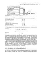
Some typical load histories for mechanical components and systems are shown
in Figure 4.21. The load (dead load, pressure, bending moment, etc.) is subject
to variation in all cases, rather than a unique value, the likely shape of the ®nal
Figure 4.21
Typical load histories for engineering components/systems
Variables in probabilistic design 169
distribution shown schematically to the right of each load history. Even permanent
dead loads that should maintain constant magnitude show a relatively small and
slow random variation in practice. At the other end of the loading type spectrum are
transient loads which occur infrequently and last for a short period of time ± an

impulse, for example extreme wind and earthquake loads (Shinozuka and Tan, 1984).
The above would assume that the load distributions for static designs are often
highly unsymmetrical, indicating that there is a small proportion of loads that are
relatively large (Bury, 1975). During the conditions of use, environmental and service
variations give rise to temporary overloads or transients causing failures (Klit et al.,
1993). Data collected from mechanical equipment in service has shown that these
transient loads developed during operation may be several times the nominal load
as shown in Figure 4.22.
There is very little information on the variational nature of loads commonly
encountered in mechanical engineering. Several references provide guidance in
terms of the coecient of variation, C
v
, for some common loading types as shown
in Table 4.9 (Bury, 1975; Ellingwood and Galambos, 1984; Faires, 1965; Lincoln
Figure 4.22
Transient loads may be many times the static load in operation (Nicholson et al., 1993)
Table 4.9 Typical coecient of variation, C
v
, for various loading
conditions
Loading condition C
v
Aerodynamic loads in aircraft 0.012 to 0.04
Spring force 0.02
Bolt pre-load using powered screwdrivers 0.03
Powered wrench torque 0.09
Dead load 0.1
Hand wrench torque 0.1
Live load 0.25
Snow load 0.26

Human arm strength 0.3 to 0.4
Wind loads 0.37
Mechanical devices in service 0.5
170 Designing reliable products
et al., 1984; Shigley and Mischke, 1996; Smith, 1995; Woodson et al., 1992). These
values are representative of the variation experienced during typical duty cycles.
These values can only act as a guide in mechanical design and should be treated
with caution and understanding, but they do indicate that loads vary quite consider-
ably, when you observe that the ultimate tensile strength, Su, of steel generally has a
C
v
 0:05. The smaller the variance in design parameters, the greater will be the
reliability of the design to deal with unforeseen events (Suh, 1990), and this would
certainly apply to the loads too due to the diculty in determining the nature of
overloading and abuse in service at the design stage.
Example ± determining the stress distribution using the coef®cient
of variation
When dimensional variation is large, its eects must be included in the analysis of the
stress distribution for a given situation. However, in some cases the eects of dimen-
sional variation on stress are negligible. A simpli®ed approach to determine the likely
stress distribution then becomes available. Given that the mean load applied to the
component/assembly is known for a particular situation, the loading stress can be
estimated by using the coecient of variation, C
v
, of the load and the mean value
for the stress determined from the stress equation for the failure mode of concern.
For example, suppose we are interested in knowing the distribution of stress
associated with the tensile static loading on a rectangular bar (see Figure 4.23). It
is known from a statistical analysis of the load data that the load, F, has a coecient
of variation C

v
 0:1. The stress, L, in the bar is given by:
L 
F
ab
Figure 4.23
Tensile loading on a rectangular bar
Variables in probabilistic design 171
where:
F  load
a and b  mean sectional dimensions of the bar:
Assuming the variation encountered in dimensions `a'and`b' is negligible, then the
mean stress, 
L
, on the bar is:

L


F

a
 
b

100 000
0:03 Â 0:05
 66:67 MPa
The load coecient of variation C
v

 0:1. Rearranging the equation for C
v
to give the
standard deviation of the loading stress yields:

L
 C
v
 
L
 0:1 Â 66:67  6:67 MPa
The stress, L, can therefore be approximated by a Normal distribution with par-
ameters:
L $ N66:67; 6:67MPa
Probabilistic considerations
For many years in mechanical design, load variations have been masked by using
factors of safety in a deterministic approach, as shown below (Ullman, 1992):
. 1 to 1.1 ± Load well de®ned as static or ¯uctuating, if there are no anticipated over-
loads or shock loads and if an accurate method of analysing the stress has been
used.
. 1.2 to 1.3 ± Nature of load is de®ned in an average manner with overloads of 20 to
50% and the stress analysis method may result in errors less than 50%.
. 1.4 to 1.7 ± Load not well known and/or stress analysis method of doubtful
accuracy.
These factors could be in addition to the factors of safety typically employed as
discussed at the beginning of this section. Because of the diculty in ®nding the
exact distributional nature of the load, this approach to design was considered
adequate and economical. It has been argued that it is far too time consuming and
costly to measure the load distributions comprehensively (Carter, 1997), but this
should not prevent a representation being devised, as the alternative is even more

reprehensible (Carter, 1986). Practically speaking, deciding on the service loads is
frequently challenging, but some sort of estimates are essential and it is often
found that the results are close to the true loads (Faires, 1965).
Since static failures are caused by infrequent large loads, as discussed above, it is
important that the distributions that model these extreme events at the right-hand
side of the tail are an accurate representation of actual load frequencies. Control of
the load tail would appear to be the most eective method of controlling reliability,
because the tail of the load distribution dictates the shape of the distribution and
hence failure rate (Carter, 1986). The Normal distribution is usually inappropriate,
although some applied loads do follow a Normal distribution, for example rocket
motor thrust (Haugen, 1965) or the gas pressure in the cylinder heads of reciprocating
engines (Lipson et al., 1967). Other loads may be skewed or possess very little scatter
172 Designing reliable products
and in fact load spectrums tend to be highly skewed to the left with high loads
occurring only occasionally as shown in Figure 4.24 (Bury, 1974). Civil engineering
structures are usually subjected to a Lognormal type of load, but in general the
Normal and 3-parameter Weibull distributions are commonly employed for mechanical
components, and the Exponential for electrical components (Murty and Naikan, 1997).
It is useful in the ®rst instance to describe the load in terms of a Normal distribution
because of the necessity to transform it into the loading stress parameters through the
variance equation and dimensional variables. Although the accuracy of the variance
equation is dependent on using to near-Normal distributions and variables of low
coecient of variation (C
v
< 0:2), it is still useful when the anticipated loads have
high coecients of variation. Even if the distribution accounting for the static load
is Normal, the stress model is usually Lognormal (Haugen, 1980) due to the complex
nature of the variables that make up the stress function.
Experimental load analysis
Information on load distributions was virtually non-existent until quite recently

although much of it is very rudimentary, probably because collecting data is very
expensive, the measuring transducers being dicult to install on the test product or
prototype (Carter, 1997). It has been cited that at least one prototype is required to
make a reliability evaluation (Fajdiga et al., 1996), and this must surely be to under-
stand the loads that could be experienced in service as close as possible.
In experimental load studies, the measurable variables are often surface strain,
acceleration, weight, pressure or temperature (Haugen, 1980). A discussion of the
techniques on how to measure the dierent types of load parameters can be found
in Figliola and Beasley (1995). The measurement of stress directly would be
advantageous, you would assume, for use in subsequent calculations to predict
reliability. However, no translation of the dimensional variability of the part could
then be accounted for in the probabilistic model to give the stress distribution. A
better test would be to output the load directly as shown and then use the appropriate
probabilistic model to determine the stress distribution.
A key problem in experimental load analysis is the translation of the data yielded from
the measurement system (as represented by the load histories in Figure 4.21) into an
Figure 4.24
A loading stress distribution with extreme events
Variables in probabilistic design 173
appropriate distributional form for use in the probabilistic calculations. Measuring the
distribution of the load peak amplitudes is a useful model for both static and dynamic
loads, as peaks are meaningful values in the load history (Haugen, 1980). A much sim-
pler method, described below, analyses the continuous data from the load history.
Assuming that the statistical characteristics of a load function, xt, are not
changing with time, then we can use the load±time plot, as shown in Figure 4.25,
to determine the PDF for xt. The ®gure shows a sample history for a random
process with the times for which x xt x  dx, identi®ed by the shaded
strips. During the time interval, T, xt lies in the band of values x to x  dx for
a total time of dt
1

 dt
2
 dt
3
 dt
4
. We can say that if T is long enough (in®nite),
the PDF or f x is given by:
f xdx  fraction of total elapsed time for which xt lies in the x to x  dx band

dt
1
 dt
2
 dt
3
 FFF
T


n
i 1
dt
i
T
4:25
The fraction of time elapsed for each increment of x can be expressed as a percentage
rounded to the nearest whole number for use in the plotting procedure to ®nd the
characterizing distributional model. Estimation of the distribution parameters and
the correlation coecient, r, for several distribution types is then performed by

using linear recti®cation and the least squares technique. The distributional model
with a correlation coecient closest to unity would then be chosen as the most
appropriate PDF representing the load history. The above can be easily translated
into a computer code providing an eective link between the prototype and load
model. See the case study later employing this technique for statistically modelling
a load history.
For discrete data resulting from many individual load tests, for example spring
force for a given de¯ection as shown in Figure 4.26, a histogram is best constructed.
The optimum number of classes can be determined from the rules in Appendix I.
Again, the best distribution characterizing the sample data can be selected using
the approach in Section 4.2.
Figure 4.25
Determination of the PDF for a random process (adapted from Newland, 1975)
174 Designing reliable products
Given the lack of available standards and the degree of diversity and types of load
application, the approach adopted has focused on supporting the engineer in the early
stages of product development with limited experimental load data.
Anthropometric data
Some failures are caused by human related events such as installation, operation or
maintenance errors rather than by any intrinsic property of the components (Klit
et al., 1993). A number of mechanical systems require operation by a human, who
thereby becomes an integral part of the system and has a signi®cant eect on the
reliability (Smith, 1976). Consumer products are notorious for the ways in which
the consumer can and will misuse the product. It therefore becomes important to
make a reasonable determination of the likely loading conditions associated with
the dierent users of the product in service (Cruse, 1997b).
Human force data is typically given as anthropometric strength. An example is
given in Table 4.10 for arm strength for males' right arms in the sitting position.
This type of data is readily available and presented in terms of the mean and standard
deviation for the property of interest (Pheasant, 1987; Woodson et al., 1992). Many

studies have been undertaken to collate this data, particularly in the US armed forces
and space programmes.
Anthropometric data is also provided for population weights. For example,
C
v
 0:18 for the weight of males aged between 18 and 70 (Woodson et al., 1992).
For English males within this age range, the mean,   65 kg, and the standard
deviation,   11:7 kg. Therefore, at 3, you would expect 1 in 1350 males in this
age range to be over 100 kg in weight, as determined from SND theory. In the US,
this probability applies to males of 118 kg in weight. The designer should use this
type of data whenever human interaction with the product is anticipated.
Frequency
Force per unit deflection
Figure 4.26
Distribution of spring force for a given de¯ection
Variables in probabilistic design 175
4.4 Stress±Strength Interference (SSI) analysis
Having previously introduced the key methods to determine the important variables
with respect to stress and strength distributions, the most acceptable way to predict
mechanical component reliability is by applying SSI theory (Dhillon, 1980). SSI
analysis is one of the oldest methods to assess structural reliability, and is the most
commonly used method because of its simplicity, ease and economy (Murty and
Naikan, 1997; Sundararajan and Witt, 1995). It is a practical engineering tool used
for quantitatively predicting the reliability of mechanical components subjected to
mechanical loading (Sadlon, 1993) and has been described as a simulative model of
failure (Dasgupta and Pecht, 1991).
The theory is concerned with the problem of determining the probability of failure
of a part which is subjected to a loading stress, L, and which has a strength, S.Itis
assumed that both L and S are random variables with known PDFs, represented
by f S and f L (Disney et al., 1968). The probability of failure, and hence the

reliability, can then be estimated as the area of interference between these stress
and strength functions (Murty and Naikan, 1997).
SSI is recommended for situations where a considerable potential for variation
exists in any of the design parameters involved, for example where large dimensional
variations exist or when the anticipated design loads have a large range. The main
reasons for performing it are (Ireson et al., 1996):
. To ensure sucient strength to operate in its environment and under speci®ed loads
. To ensure no excess of material or overdesign occurs (high costs, weight, mass,
volume, etc.).
Some advantages and disadvantages of SSI analysis have also been summarized
(Sadlon, 1993):
Table 4.10 Human arm strength data (Woodson et al., 1992)
Direction of force Elbow angle Mean force  (N) Standard deviation  (N)
Push 608 410 169
908 383 147
1208 459 192
1508 548 201
1808 615 218
Pull 608 281 103
908 392 134
1208 464 138
1508 544 161
1808 535 165
176 Designing reliable products
Advantages:
. Addresses variability of loading stress and material strength
. Gives a quantitative estimate of reliability.
Disadvantages:
. Interference is often at the extremes of the distribution tails
. The stress variable is not always available.

4.4.1 Derivation of reliability equations
A mechanical component is considered safe and reliable when the strength of the
component, S, exceeds the value of loading stress, L, on it (Rao, 1992). When the
loading stress exceeds the strength, failure occurs, the reliability of the part, R,
being related to this failure probability, P, by equation 4.26:
PS > LR 4:26
It is also evident that the reliability can also be derived by ®nding the probability of
the loading stress being less than the strength of the component:
PL < SR 4:27
This is demonstrated graphically in Figure 4.27 which shows the loading stress
remains less than some given value of allowable strength (Haugen, 1968; Rao,
1992). The probability of a strength S
1
in an interval dS
1
is:
PS
1
ÿ
dS
1
2
S S
1

dS
1
2

 fS

1
dS
1
 A
1
4:28
The probability of occurrence of a loading stress less than S
1
is:
PL< S
1


S
ÿI
fLdL  FLA
2
4:29
Figure 4.27
SSI theory applied to the case where loading stress does not exceed strength
Stress±Strength Interference (SSI) analysis 177
The probability of these two events occurring simultaneously is the product of
equations 4.28 and 4.29 which gives the elemental reliability, dR, as:
dR  fS
1
dS
1
Á

S

ÿI
fLdL 4:30
For all possible values of strength, the reliability, R, is then given by the integral:
R 

dR 

I
ÿI
f S

S
ÿI
f LdL

dS 4:31
This equation can be simpli®ed by omitting negative limits to give the general
equation for reliability using the SSI approach. For static design (i.e. no strength
deterioration) with a single application of the load, equation 4.31 becomes:
R 

I
0
f S

S
0
f LdL

dS 4:32

When the loading stress can be determined by a CDF in closed form, this simpli®es to:
R 

I
0
FLÁ f SdS 4:33
In general both the load and strength are functions of time more often than not
(Vinogradov, 1991); however, in general mechanical engineering the control of the
operation is more relaxed and so it becomes more dicult to de®ne a duty cycle
(Carter, 1997). However, in most design applications the number of load applications
on a component/system during its contemplated life is a large number (Bury, 1975)
and this has a major eect on the predicted reliability. The time dependence of the
load becomes a factor that transforms a problem of probabilistic design into one of
reliability. The reliability after multiple independent load applications in sequence,
R
n
, is given by:
R
n


I
0
f S

S
0
f LdL

n

dS 4:34
where:
n  number of independent load applications in sequence
or from equation 4.33:
R
n


I
0
FL
n
Á f SdS 4:35
Equation 4.34 represents probably one of the most important theories in reliability
(Carter, 1986). The number of load applications de®nes the useful life of the compo-
nent and is of appropriate concern to the designer (Bury, 1974). The number of times
a load is applied has an eect on the failure rate of the equipment due to the fact that
the probability of experiencing higher loads from the distribution population has
increased. Each load application in sequence is independent and belongs to the
same load distribution and it is assumed that the material suers no strength
178 Designing reliable products
deterioration. In fact, the strength distribution would change due to the elimination
of the weak items from the population, and would in eect become truncated at the
left-hand side. However, no account of strength alteration with time is included in any
of the approaches discussed. Monte Carlo simulation can be used to demonstrate this
principle, as well as providing another means of solving the general reliability equa-
tion. However, the major shortcoming of the Monte Carlo technique is that it requires
a very large number of simulations for accurate results and is therefore not suited to
low probability levels (Lemaire, 1997).
If we had taken the case where the strength exceeds the applied stress, this would

have yielded a slightly dierent equation as shown below:
R 

I
0
f L

I
L
f SdS

dL 4:36
This can also be simpli®ed when the strength CDF is in closed form to give:
R  1 ÿ

I
0
FSÁ f LdL 4:37
4.4.2 Reliability determination with a single load application
Analytical solutions to equation 4.32 for a single load application are available for
certain combinations of distributions. These coupling equations (so called because
they couple the distributional terms for both loading stress and material strength)
apply to two common cases. First, when both the stress and strength follow the
Normal distribution (equation 4.38), and secondly when stress and strength can be
characterized by the Lognormal distribution (equation 4.39).
Figure 4.28 shows the derivation of equation 4.38 from the algebra of random
variables. (Note, this is exactly the same approach described in Appendix VIII to
®nd the probability of interference of two-dimensional variables.)
z ÿ


S
ÿ 
L


2
S
 
2
L
q
4:38
where:
z  Standard Normal variate

S
 mean material strength

S
 material strength standard deviation

L
 mean applied stress

L
 applied stress standard deviation:
z ÿ
ln

S


L

1  C
2
L
1  C
2
S
s
23

ln 1  C
2
L
1  C
2
S

ÂÃ
q
4:39
Stress±Strength Interference (SSI) analysis 179
where:
C
L


L


L
and C
S


S

S
(the mean and standard deviation determined
from Appendix IX):
Using the SND theory from Appendix I, the probability of failure, P, can be deter-
mined from the Standard Normal variate, z, by:
P  È
SND
z4:40
The reliability, R, is therefore:
R  1 ÿ P  1 ÿ È
SND
z4:41
Using the Normal distribution to model both stress and strength is the most common
and the mathematics is easily managed, giving a quick and economical solution. The
convenience and ¯exibility of using a single distribution, such as the Normal, is very
attractive and has found favour with many practitioners. However, it has been
observed that loading stresses and material strengths do not necessarily follow the
Figure 4.28
Derivation of the coupling equation for the case when both loading stress and material strength
are a Normal distribution
180 Designing reliable products
Normal or Lognormal distributions. For the purposes of SSI theory, the 3-parameter
Weibull distribution is dicult to work with. The probability of failure cannot be

obtained by coupling equations. This means that we need more general approaches
to solve the SSI problem for any combination of distribution. One such approach
is the Integral Transform Method (Haugen, 1968). The integral transform method
starts by replacing the terms in equation 4.36 with the following:
G 

I
L
f SdS 4:42
and
H 

I
L
f LdL 4:43
By determining dH  f LdL, this changes the limits of integration to 0 to 1, as
shown in Figure 4.29, to give the reliability, R,as:
R 

1
0
GdH 4:44
or
R  1 ÿ

1
0
HdG 4:45
Equation 4.44 is solved using Simpson's Rule to integrate the area of overlap. The
method is easily transferred to computer code for high accuracy. See Appendix XII

for a discussion of Simpson's Rule used for the numerical integration of a function.
Equation 4.44 permits the calculation of reliability for any combinations of distribu-
tions for stress and strength provided the partial areas of G and H can be found.
For the general SSI method, its accuracy relies on evaluating the areas under the
functions and the numerical methods employed. However, the integral transform
1
0
1
Reliability
Figure 4.29
Plot of G versus H for the integral transform method
Stress±Strength Interference (SSI) analysis 181
method has also been applied to cases where no basis exists for assuming any speci®c
distributions for either stress or strength, but where experimentation has been per-
formed yielding sucient empirical data (Kapur and Lamberson, 1977; Verma and
Murty, 1989).
4.4.3 Reliability determination with multiple load application
The approach taken by Carter (1986, 1997) to determine the reliability when multiple
load applications are experienced (equation 4.34) is ®rst to present a Safety Margin,
SM, a non-dimensional quantity to indicate the separation of the stress and strength
distributions as given by:
SM 

S
ÿ 
L


2
S

 
2
L
q
4:46
This is essentially the coupling equation for the case when both stress and strength are
a Normal distribution. A parameter to de®ne the relative shapes of the stress and
strength distributions is also presented, called the Loading Roughness, LR, given by:
LR 

L


2
S
 
2
L
q
4:47
The typical loading roughness for mechanical products is high, typically 0.9 (Carter,
1986). A high loading roughness means that the variability of the load is high com-
pared with that of the strength, but does not necessarily mean that the load itself is
high (Leitch, 1995) (see Figure 4.30). The general run of mechanical equipment is
subject to much rougher loading than, say, electronic equipment, although it has
been argued that electronic equipment can also be subjected to rough loading
under some conditions (Loll, 1987). It arises largely due to the less precise knowledge
and control of the environment, and also from the wide range of dierent applications
of most mechanical components. An implication of this is that the reliability of the
system is relatively insensitive to the number of components and the reliability of

mechanical systems is determined by its weakest link (Broadbent, 1993; Carter,
1986; Furman, 1981; Roysid, 1992). It also means that the probability of failure
per application of load at high SM and LR values where `n' is much greater than 1
is very close to that for single load applications. For this reason, Carter (1986)
notes that it is impossible to design for a speci®ed reliability with lower LR values.
For a given SM, LR and duty cycle, n (as de®ned by the number of times the load is
applied), the failure per application of the load, p, can be determined from Figure
4.31. The ®gure has been constructed for near-Normal stress and strength interference
conditions and where `n' is much greater than 1. The ®nal reliability is given by
(O'Connor, 1995):
R
n
1 ÿ p
n
4:48
where:
p  probability of failure per application of load `n':
182 Designing reliable products
Bury (1974; 1975; 1978; 1999) introduces the concept of duty cycles to static design in
a dierent approach. The duty cycle or mission length of a design is equivalent to the
number of load applications, n; however, it is only the maximum value which is of
design signi®cance. If the load, L, is a random variable then so is its maximum
value,

L, and the PDFs of each are related. It can be shown that the CDF, F

L,
of the maximum among `n' independent observations on L is:
G
n



LF

L
n
4:49
G
n


L is often dicult to determine for a given load distribution, but when `n' is large,
an approximation is given by the Maximum Extreme Value Type I distribution of the
maximum extremes with a scale parameter, Â, and location parameter, . When the
initial loading stress distribution, f L, is modelled by a Normal, Lognormal, 2-par-
ameter Weibull or 3-parameter Weibull distribution, the extremal model parameters
can be determined by the equations in Table 4.11. These equations include terms for
the number of load applications, n. The extremal model for the loading stress can then
be used in the SSI analysis to determine the reliability.
For example, to determine the reliability, R
n
, for `n' independent load applications,
we can use equation 4.33 when the loading stress is modelled using the Maximum
Extreme Value Type I distribution, as for the above approach. The CDF for the
Figure 4.30
Relative shape of loading stress and strength distributions for various loading roughnesses and
arbitrary safety margin
Stress±Strength Interference (SSI) analysis 183
Figure 4.31
Failure probability (per application of load) versus safety margin for various loading roughness

values (adapted from Carter, 1997)
Table 4.11 Extremal value parameters from initial loading stress distributions
Initial loading stress
distribution
Location parameter () Scale parameter (Â)
Normal  

2lnnÿ0:5lnlnnÿ1:2655

2lnn
p
!


2lnn
p
Lognormal exp  Á z
z  Â
ÿ1
SND

1 ÿ
1
n

 Á 

1
n


1

2
p
exp

ÿ
z
2
2

H
f
f
f
d
I
g
g
g
e
2-parameter Weibull
 ! 1
lnn
1=




lnn

1 ÿ=
3-parameter Weibull xo  ÿxolnn
1=

 ÿxo


lnn
1 ÿ=
 ! 1
184 Designing reliable products