Experimental Business Research II springer 2005 phần 4 ppsx

CHOOSING

A

MODEL

OUT OF
F

MANY POSSIBLE ALTERNATIVES
Y
E

67

In our double auction experiment, marginal abatement costs converged less
rapidly than in the bilateral trading setting. We conjecture that this arises because
at most one pair in the double auction can trade at the same time while at most three
pairs can do so under bilateral trading.
In order to understand how much market power a country has, we need an
aggregate excess demand curve of all the subjects regarding the marginal abatement
cost curves as the excess demand curves for emissions allowances. In our design, the
competitive equilibrium price range is from 118 to 120, while the excess demand for
permits is zero under this price range. Each country might be able to change the
equilibrium price by increasing (or decreasing) the quantity supplied (or demanded).
If so, and the surplus of this country under the new equilibrium price is greater than
the surplus under the true equilibrium price. Then we say that the country has market
power. After careful examination, we find that the only country that has market
power in our design is the US. Table 3 shows that the benefits of the US were more
than three times larger than the benefit at the competitive equilibrium in two out of
eight sessions under bilateral trading. A statistical test shows that the US did not

exercise its market power in any session. Most probably, the subjects could not exploit
the marginal abatement cost curve information to use their market power. Under
double auction, the individual efficiency of the US is statistically greater than one.
It is remarkable to find that high efficiency was observed even when there
existed a subject who had market power. What would happen if subjects could easily
find out that they have some market power and the transaction is done by double
auction? Bohm (2000) found that the efficiency in this setting is still high, but the
distribution of the surplus is distorted. That is, it is often said that the efficiency of
the market would be damaged when there are countries that have market power, but
this is not confirmed in laboratory experiments. It seems that the double auction
and the typical explanation of a monopoly are totally different from each other. In
a textbook theory of monopoly, a monopolist offers a price to every buyer, and a
buyer must accept or reject the price. The second point is that a country that is
supposed to be a seller under the competitive equilibrium price would be a buyer if
the price of permits were considerably low.
Consider the policy implications of Hizen and Saijo’s experiment. If the main
target of a policy maker is efficiency in achieving the Kyoto target, both bilateral
trading and the double auction can attain this goal. If the policy maker’s target is to
achieve equity so that the same permits must be traded at the same price, the double
auction is better than bilateral trading. If market power is not exercised, then it
seems that bilateral trading is better than the double auction. If the policy maker
believes that the information transaction takes a considerable amount of resources,
then the double auction is better than bilateral trading.
Hizen, Kusakawa, Niizawa and Saijo (2000) focus on two assumptions that are
employed by Hizen and Saijo (2001). The first is that the starting point of the
transaction in Hizen and Saijo is the assigned amount of the Kyoto target. The second
is that a country can move on the marginal abatement cost curve freely. This assumption is made to avoid the non-compliance problem. In Hizen, Kusakawa, Niizawa


68

Experimental Business Research Vol. II

and Saijo’s (2000) experiment, the starting point of the transaction becomes more
realistic as a circle on the marginal cost curve shown in Figure 5. Furthermore, they
impose two restrictions on the movement on the marginal cost curve. A country can
move on it from right to left, but not in the opposite direction. Once a country
spends resources for abatement, it cannot reduce its marginal abatement costs through
increased emissions. This corresponds to investment irreversibility. Once an agent
invests some resources, the agent cannot go back to the original position. The second
restriction is a condition on the decision making on domestic abatement. During
60 minutes of transactions, a country must decide on its domestic abatement decision within half an hour. This reflects that it takes a considerable amount of time to
reduce emissions after the decision is made. On the other hand, emissions trading
can be conducted any time during the 60 minutes. Under these new conditions, a
country might not be able to attain the assigned amount of emissions. If this is the
case, then the country must pay a penalty of $300 per unit. This is considerably high
since the competitive equilibrium price range is from $118 to 120.
In Hizen, Kusakawa, Niizawa, and Saijo’s (2000) experiment, the marginal abatement cost curves are private information. The trading methods are bilateral trading
and double auction. In bilateral trading, the control is the disclosure of contract price
information (O) or the concealment of this information (X). In the double auction,
this information is automatically revealed to everyone. The rest of the design is the
same as in Hizen-Saijo’s experiment.
Table 4 is similar to Table 3. Let us explain the two numbers under the name of
each country. The US has (55, 50), for example, indicating that the initial point is 55
and the competitive equilibrium point after the transaction is 50 (Figure 5). Now,
consider the two numbers in the data. The numbers for the US in session O4
in bilateral trading is (23, −2). The first number shows that the US conducted 32
(= 55 − 23) units of domestic reduction, which resulted in 23 units on the horizontal
axis by moving the marginal abatement cost curve. In order to comply with the
Kyoto target, the US must buy at least 23 units of emissions permits, but since

the US bought 25 units, this resulted in −2 on the horizontal axis. That is, the US
achieved 2 units of over-compliance.
We have two kinds of efficiency. The first is the actual efficiency attained.
That is, actual efficiency measures the actual surplus attained in each experiment
after assigning a zero value to units of over-compliance and $300 for each unit of
non-compliance as $300. This is shown in the bottom row of Table 5. For example,
the actual surplus of session O4 is 5736 and its efficiency is 0.821. The second kind
of efficiency is the modified efficiency that reevaluates units of over-compliance and
units of non-compliance by using the concept of opportunity costs. Details are given
in Hizen, Kusakawa, Niizawa, and Saijo (2000). This is shown underneath the box
in Table 5. For example, the modified surplus of session O4 is 6596 and its modified
efficiency is 0.944. The average efficiency (the modified efficiency) in the X sessions is 0.605 (0.811); in the O sessions it is 0.502 (0.807); and in the D sessions it
is 0.634 (0.873).
After a careful look at Table 5, we make the following observation.


100
0.256
−10, 0
375
0.605
10, 0

5600
0.801
6230
0.891

1046
1.715

23, 0

240
0.615
−5, 0

−650
−1.048
5, −5

2175
1.426
35, 0

5112
0.731

5612
0.803

2 (1290)
(Ukraine)
(−10)(−30, 0)

3 (610)
(U.S.A.)
(55)(50, 0)

4 (390)
(Poland)

(−5)(−10, 0)

5 (620)
(EU)
(25)(20, 0)

6 (1525)
(Japan)
(40)(25, 0)

Sum (6990)

2130
1.397
25, 0

850
1.371
20, 0

94
0.241
−10, 0

1416
2.321
23, 0

6686
0.957

384
0.150
−52, 0

O2

−4130
−6.770
−20, −30

2040
1.338
25, 0

975
1.573
20, 0

6680
0.956

−270
−0.039
3140
0.449

2430
0.348

1931
1.266
35, 0

1002
1.616
20, 0

500
1.282
−10, 0

−4094
−6.711
50, 23

−565
−0.438
−20, −15

77
0.197
−10, 0

2625
2.035
−20, 0

1415
0.554

−55, −3

O1

6146
0.879

1625
1.066
25, 0

630
1.016
20, 0

300
0.769
−13, 0

481
0.789
23, 0

1285
0.996
−25, 0

1825
0.714
−33, 0

O3

6596
0.944

5736
0.821

340
0.223
30, −5

965
1.556
20, −2

450
1.154
−10, 0

316
0.518
23, −2

2200
1.705
−20, 0

1465

0.573
−52, 0

O4

6950
0.994

2515
1.649
35, 0

760
1.226
20, 0

165
0.423
−10, 0

890
1.459
40, 0

1195
0.926
−30, 0

1425
0.558

−55, 0

D1

5856
0.838

2446
0.350

25
0.016
25, −10

−900
−1.452
10, −10

275
0.705
−10, 0

641
1.051
23, 0

−30
−0.023
−30, −27

2435
0.953
−65, 0

D2

6426
0.919

5946
0.851

1822
1.195
25, −5

770
1.242
20, 0

375
0.962
−11, 0

769
1.261
23, 0

850
0.659

−20, 0

1360
0.532
−44, 0

D3

5186
0.742

2376
0.340

1200
0.787
25 , 0

682
1.100
20, 0

763
1.956
−17, 0

−404
−0.662
23, 0

−1925
−1.492
−30, −37

2060
0.806
−60, 0

D4

MANY POSSIBLE ALTERNATIVES
Y
E

4136
0.592

5426
0.776

−3100
−2.033
15, −25
766
0.110

1710
0.245
35, 6

850
1.371
25, 0

20
0.051
−17, 0

556
0.911
23, 0

700
0.543
−20, 0

656
0.257
−42, 0

X4

OUT OF
F

220
0.361
30, 3

1820

1.411
−30, 0

620
0.243
−65, −22

X3

MODEL

1175
0.911
−20, 0

766
0.594
−28, 0

1 (2555)
(Russia)
(−32)(−55, 0)
1600
0.626
−32, 0

X2

1535
0.601

−40, 0

X1

Double Auction
A

Subject No.

Bilateral Trading

Table 5. Efficiencies in the Hizen, Kusakawa, Niizawa, and –Saijo’s (2000) experiment

CHOOSING
69


70

Experimental Business Research Vol. II
Country 1

Country 2

MAC

P*

MAC
Country

1’s MAC
<sell>

Position after
Domestic
Reduction

Country 2’s
MAC

Position after
Domestic Reduction
<buy>

P*
P**
01

Emissions
Assigned Amount

2

Emissions
Assigned Amount

Figure 8. Point Equilibrium

Observation 7.
(1) Russia’s domestic reductions were not enough in bilateral trading, but they were

close to the domestic reduction at competitive equilibrium in the double auction.
(2) The US conducted excessive domestic reductions in all sessions.
(3) In bilateral trading, nine cases of over-compliance and three cases of noncompliance out of 48 cases were observed. On the hand, in the double auction,
five cases of over-compliance and no case of non-compliance out of 24 cases were
observed.
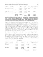
In order to understand the nature of investment irreversibility, Hizen, Kusakawa,
Niizawa, and Saijo (2000) introduced a point equilibrium. In Figure 8, the competitive equilibrium price is P*. If country 2 continues to climb the marginal abatement
cost curve, the price that equates the quantity demanded and the quantity supplied
should go down and it should be P**. We call this “should be” price the point
equilibrium price. Even though the point equilibrium price is P**, countries might
have been trading permits at a higher price than P*.
In each session, we have two pieces of price sequence data. One is the actual
price, and the other is the point equilibrium price. With the help of the point equilibrium price, we found two types of price dynamics. The first is the early point
equilibrium price decrease case (or type 1), and the second is the constant point
equilibrium price case (or type 2). We observed five sessions of type 1 and seven
sessions of type 2 out of 12 sessions.
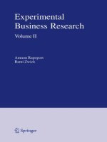
Figure 9 shows two graphs of type 1 and type 2 price dynamics. The top picture
shows a typical case of type 1 and the bottom a typical case of type 2. The horizontal
axis indicates minutes, and the vertical axis prices. The horizontal line indicates the
competitive equilibrium price, and the dark step lines indicate the point equilibrium
prices. A box indicates a transaction. The left-hand side is the seller’s name; the right
hand side is the buyer’s name; and the bottom number indicates the number of units
in the transaction. A diamond indicates the domestic reduction. Consider the top graph
that is for session D2. Up until 15 minutes, we observe many diamonds that indicate


CHOOSING

A

MODEL

OUT OF
F

MANY POSSIBLE ALTERNATIVES
Y
E

71

Price
280
260

D2

J

R: Russia P: Poland U A
10
U: Ukraine E: EU
J: Japan U sold 10
A: USA
units to A

240
220
200

5
J conducted 5 units
of domestic reduction

180
160

AJ
U JR J
10 R E
10 15
2
20
5
E
0
R A 10 J R UA
A
2
1 0
30 P A
1010 10 25
5
A U
R
A
R
5
E 5 J 5 23
Discrepancy 2 5

2
P
5
Area
10

140
120
100
80
60
40

The Early Price Decrease Case
Permit surplus: 47

20
0

R

0

5

10

15

20

25

30
35
Minutes

Price
280
260
D1
R: Russia P: Poland
240
U: Ukraine E: EU
220
J: Japan
A: USA
200
180
160
140
U A
1
10 A
R J
P AE AL A
10
0
120
10 U J 5 10 5R E

10
R AU A10 U
AU
R EP J
5 5
A 10
15
100
5 5
J
R 5 10 R
E R
3 P
80 R 20 J 5
10 5
U
5
60
10
40
20
0
0
5
10
15
20
25
30
Minutes

40

45

5

U

50

55

60

J

A
10
U sold 10
units to A
U

5
J conducted 5 units
of domestic reduction

J BU E
BU
5 5

The Constant Price Case
Permit surplus: 0

35

40

45

50

Figure 9. Price Dynamics of Hizen, Kusakawa, Niizawa, and Saijo’s experiment

55

60


72

Experimental Business Research Vol. II
(1) The Early Point Equilibrium Price
Decrease Case

1600

Discrepancy Area

1400

1200

44.9%
O1
(–3.9%)

83.8%
D2
(35.0%)

1000
800
600
400
200
0
0.00

59.2%
X3
(11.0%)

91.9%
D3
(85.1%)

74.2%
D4
(34.0%)

94.4%
O4
(82.1%)
87.9%
95.7%
O3
X4
(2) The Constant Point
80.3%
(77.6%)
Equilibrium Price Case
q
X1
99.4%
0.20
0.40
0.60 (73 1%) 0.80
0 (73.1%)
1
1.00 D1
89.1%
89 1%
Modified Efficiency
X2 95.6%
(80.1%) O2
(34.8%)

Figure 10. The Relationship between Modified Efficiency and the Discrepancy Area

domestic reduction. This reduction seems to come from fear of non-compliance of

demanders. This causes the the transaction price to be higher. Even after the point
equilibrium price decreased after 10 minutes, the actual transaction prices were considerably higher than point equilibrium prices. That is, high price inertia was observed.
After half an hour, no domestic reduction was possible and the point equilibrium
becomes zero. We measured the area between the competitive equilibrium price line
and the point equilibrium price curve up to half an hour as the discrepancy area.
In the case of the bottom graph, the starting price was relatively low. Due to
this low price, supply countries did not conduct enough domestic reduction. After
10 minutes and until 30 minutes, the demand countries conducted considerable
domestic reduction. In this case, the point equilibrium price curve coincided with
the competitive equilibrium price line. That is, the discrepancy area was zero.
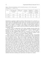
Figure 10 illustrates the relationship between the modified efficiency and the
discrepancy area. By cluster analysis, we have found two groups, type 1 and type 2.
Although the number of sessions was quite small, within the same type, it seems that
efficiencies of the double auction were higher than those of bilateral trading and
that information disclosure increased the efficiency. Summarizing these findings,
we make the following observation:
Observation 8.
(1) Two types, i.e., the early point equilibrium price decrease case and the constant
point equilibrium price case were observed.


CHOOSING

A

MODEL

OUT OF
F

MANY POSSIBLE ALTERNATIVES
Y
E

73

(2) Excessive domestic reduction was observed in both types.
(3) In both types, efficiencies in the double auction were higher than those in bilateral trading.
(4) In type 1, we observed high price inertia and a sudden price drop.
(5) In type 2, insufficient domestic reduction from the supply countries caused excessive domestic reduction from the demand-countries.
The sudden price drop observed in Observation 8–(4) would be overcome by
banking, which is allowed in the Kyoto Protocol. Muller-Mestelman (1998) found
that banking of permits had some power to stabilize the price sequence. Furthermore, under either trading rule, early domestic reduction resulted in type 1 and
caused a efficiency lower than that of type 2. It seems that haste makes waste.
6. EXPERIMENTAL APPROACH (2)
This section describes the experimental results of Mitani, Saijo, and Hamaguchi
(1998) who studied the Mitani mechanism. In their experiment, they specify cost
C1(z) and C2(z), as follows.
C1(z) = 37.5 + 0.5(5 + z)2, C2(z) = 15z − 0.75z 2.
Furthermore, the penalty function of country 1 is specified by
d p p2 )

⎧0 if p
⎨
⎩K if p

p2
p2

, where K > 0.

Thus, if countries 1 and 2 announce the same price, then the penalty is zero; if not,
then the fixed amount of penalty is imposed on country 1. Therefore, the payoff
functions of the mechanism become
g1(z, p1, p2 ) = −C1(z) + p2 z − d(p1, p2 ).
g2 (z, p1) = C2 (z) − p1z
Even with modification of the Mitani mechanism, the subgame perfect equilibrium
would not be changed. Applying the condition of subgame perfect equilibrium to the
Mitani mechanism, p1 = p2 = C′(z) = C′(z), we have C′ = 5 + z, C′ = 15 − 1.5z, and
C2
C2
1
1
hence z = 4. That is, p1 = p2 = 9.
The experimental test of the Mitani mechanism is designed so that each agent is
supposed to minimize the cost. Therefore, by putting a minus sign in the payoff of
country 1, we have
The total cost of country 1 = 37.5 + 0.5 × (5 + the units of transaction)2 − (the price
that country 2 chose) × (the units of transaction) + the charge,


74

Experimental Business Research Vol. II

where the charge term is d(p1, p2 ). We regard the payoff of country 2 as the surplus
accruing from buying emissions permits from x* to the assigned amount (Z2) as
*
2
shown in Figure 2. On the other hand, in the Mitani, Saijo, and Hamaguchi’s

*
experiment, the sum of the cost-reducing emissions from Y 2 to x* and the payment
2
p*(x* − Z 2 ) for emissions are the total cost. This does not change the subgame
2
perfect equilibrium of the Mitani mechanism since it merely changes the starting
point for either the payoff or cost. When Y 2 = 10, C2 (10) − C2(z) = 75 − 15z + 0.75z 2
= 0.75(10 − z)2 is the cost of reducing the amount of emissions from Y 2 to x*.
2
That is,
The total cost of country 2 = 0.75 × (10 − the units of transaction)2 + (the price that
country 1 chose) × (the units of transaction).
When no transaction occurs, the total cost of country 1 is 37.5 + 0.5 × 52, which
equals 50 and the total cost of country 2 is 0.75 × 102, which is 75, where the charge
term is zero.
Let us review the experiment. Two sessions were conducted, one for K = 10 and
the other for K = 50. Each session included 20 subjects who gathered in a classroom
and divided into 10 pairs. Each subject could not identify the other dyad member.
During the experiment, “emissions trading” were not used. Country 1 in the above
corresponded to subject A, and country 2 to subject B. The experimenter allotted
5 units of production to Subject A and 10 units to subject B. Then the transaction
of allotted units of production was conducted by a certain rule (i.e., the Mitani
mechanism). The allotted amounts corresponded to the reduction amounts in theory.
In order to prepare an environment in which one subject ( ) knew the production
(A
cost structure of the other subject (B), we explained the production cost to both
subjects, and then conducted four practice rounds. Two were for subject A and two
for subject B. Right before the real experiment, we announced who was subject A
and who was B. Once the role of the subjects was determined, it remained fixed
across 20 rounds.

Table 6 displays the total cost tables for subject A. The upper table is the payoff
table for subject A. The payoff for subject A is determined by pB, announced by
subject B and the amount of transaction, z, by subject A without considering the
charge term. If the prices announced by both subjects were different, subject A paid
the charge. Subject A could also see the payoff table for subject B, which is shown
in the bottom table in Table 6. The payoff for subject B is determined by pA and z is
announced by subject A. That is, subject B cannot change his or her own payoff by
changing pB. We will find the subgame perfect equilibrium through Table 6. Subject
A first solves the optimization problem in stage 2 and then chooses a z that minimizes the total cost of subject A depending on the announcement of pB by subject B.
This is z = z( pB). For example, if pB = 6, then z = 1. The diagonal from the upper left
to the bottom right corresponds to z = z( pB) in Table 6. In stage 1, subject A should
announce pA = 6, since pB = 6, to avoid the charge. However, these announcements
are not a subgame perfect equilibrium. When pA = 6, z = 6 makes the cost of subject


47.5

52.5

57.5

62.5

2

3

4

5

72.5

77.5

82.5

87.5

92.5

97.5

102.5

107.5

112.5

7

8

9

10

11

12

13

14

15
84.5

81.5

78.5

75.5

72.5

69.5

66.5

63.5

60.5

57.5

54.5

51.5

48.5

45.5

42.5

72

70

68

66

64

62

60

58

56

54

52

50

48

46

44

42

−2

60.5

59.5

58.5

57.5

56.5

55.5

54.5

53.5

52.5

51.5

50.5

49.5

48.5

47.5

46.5

45.5

−1

50

50

50

50

50

50

50

50

50

50

50

50

50

50

50

50

0

40.5

41.5

42.5

43.5

44.5

45.5

46.5

47.5

48.5

49.5

50.5

51.5

52.5

53.5

54.5

55.5

1

32

34

36

38

40

42

44

46

48

50

52

54

56

58

60

62

2

24.5

27.5

30.5

33.5

36.5

39.5

42.5

45.5

48.5

51.5

54.5

57.5

60.5

63.5

66.5

69.5

3

18

22

26

30

34

38

42

46

50

54

58

62

66

70

74

78

4

12.5

17.5

22.5

27.5

32.5

37.5

42.5

47.5

52.5

57.5

62.5

67.5

72.5

77.5

82.5

87.5

5

8

14

20

26

32

38

44

50

56

62

68

74

80

86

92

98

6

4.5

11.5

18.5

25.5

32.5

39.5

46.5

53.5

60.5

67.5

74.5

81.5

88.5

95.5

102.5

109.5

7

2

10

18

26

34

42

50

58

66

74

82

90

98

106

114

122

8

0.5

9.5

18.5

27.5

36.5

45.5

54.5

63.5

72.5

81.5

90.5

99.5

108.5

117.5

126.5

135.5

9

0

10

20

30

40

50

60

70

80

90

100

110

120

130

140

150

10

MANY POSSIBLE ALTERNATIVES
Y

E

98

94

90

86

82

78

74

70

66

62

58

54

50

46

42

39.5

−3

OUT OF
F

67.5

42.5

1

38

−4

MODEL

6

37.5

0

−5

Your Choice of transaction (A)

Table 6. The total cost table for Subject A under the Mitani Mechanism

A

B’s choice of price

CHOOSING
75


Your (A) choice of price

168.8

163.8

158.8

153.8

148.8

143.8

138.8

133.8

128.8

123.8

118.8

113.8

108.8

103.8

98.8

93.8

1

2

3

4

5

6

7

8

9

10

11

12

13

14

15

−5

0

Table 6. (cont’d)

87

91

95

99

103

107

111

115

119

123

127

131

135

139

143

147

−4

81.8

84.8

87.8

90.8

93.8

96.8

99.8

102.8

105.8

108.8

111.8

114.8

117.8

120.8

123.8

126.8

−3

78

80

82

84

86

88

90

92

94

96

98

100

102

104

106

108

−2

75.8

76.8

77.8

78.8

79.8

80.8

81.8

82.8

83.8

84.8

85.8

86.8

87.8

88.8

89.8

90.8

−1

75

75

75

75

75

75

75

75

75

75

75

75

75

75

75

75

0

75.8

74.8

73.8

72.8

71.8

70.8

69.8

68.8

67.8

66.8

65.8

64.8

63.8

62.8

61.8

60.8

1

78

76

74

72

70

68

66

64

62

60

58

56

54

52

50

48

2

81.8

78.8

75.8

72.8

69.8

66.8

63.8

60.8

57.8

54.8

51.8

48.8

45.8

42.8

39.8

36.8

3

87

83

79

75

71

67

63

59

55

51

47

43

39

35

31

27

4

Your Choice of transaction (A)

93.8

88.8

83.8

78.8

73.8

68.8

63.8

58.8

53.8

48.8

43.8

38.8

33.8

28.8

23.8

18.8

5

102

96

90

84

78

72

66

60

54

48

42

36

30

24

18

12

6

111.8

104.8

97.8

90.8

83.8

76.8

69.8

62.8

55.8

48.8

41.8

34.8

27.8

20.8

13.8

6.8

7
3

123

115

107

98

90

82

74

66

58

50

42

34

26

19

11

8

135.8

126.8

117.8

108.8

99.8

90.8

81.8

72.8

63.8

54.8

45.8

36.8

27.8

18.8

9.8

0.8

9

150

140

130

120

110

100

90

80

70

60

50

40

30

20

10

0

10

76
Experimental Business Research Vol. II


CHOOSING

A

MODEL

OUT OF
F

MANY POSSIBLE ALTERNATIVES
Y
E

77

70

Total Cost

60

A’s Total Cost

50

B’s Total Cost

40

A’s Total Cost at
Subgame perfect
eq.
B’s Total Cost at
subgame perfect

30
20
10
1 2 3 4 5 6 7 8 9 10 11 12 13 14 15 16 17 18 19 20
Rounds

Figure 11. Average Total Costs when the charge is 10

B the minimum. Then, subject B would choose pB = 11 since subject B incorporates
the behavior of subject A, that is, z = z( pB). Therefore, z = 1 and pA = 6 are not the
best responses to subject A since subject A could avoid the charge by announcing
pB = 11. That is, z = 1 and pA = pB = 6 are not a subgame perfect equilibrium. Consider now that subject B announces pB = 9. Then, subject A would choose z = 4
so that subject A could minimize his or her total cost. On the other hand, subject
B would announce pA = 9, which is the same as the announcement of subject A.
Then, subject B would notice that z = 4 would minimize the total cost under pA = 9.
In order for subject A to choose z = 4, subject B announces pB = 9 taking into
account z = z( pB). That is, z = 4 and pA = pB = 9 are the subgame perfect equilibrium.
The total cost is 42 for subject A and 63 for subject B.
Figure 11 shows the average total costs of subjects A and B when the charge is
10. They are smaller than those at subgame perfect equilibrium and they decrease
with experience. We therefore make the following observation:
Observation 9. When the charge is 10, the average total costs of subjects A and B
are smaller than those at the subgame perfect equilibrium, they decreases with experience, and no pair who played subgame perfect equilibrium strategies was found.
Why does the subject not adhering to subgame perfect equilibrium play? In early
rounds, subjects noticed from Table 6 that a strategy profile of z = 10, pA = 0, and
pB = 15 made subject A’s cost 10 and subject B’s cost 0. Under this strategy profile,
subject A’s cost is 0, but he or she must pay the charge since the two prices are not
the same. Notice further that this profile is not a Nash equilibrium because subject
A could avoid the charge by announcing pA = 15. Consider the implication of this

strategy profile. Subject A can make the purchasing price of emissions permits for
subject B free of charge, and subject B can make the selling price of them for subject A as high as possible. Our highest price in Table 1 is 15. At the same time,


78

Experimental Business Research Vol. II

the profile maximizes the number of transactions. Although subject A must pay the
charge, the payoff profile of this strategy profile is strictly Pareto superior to the
payoff profile at the subgame perfect equilibrium. We found 6 pairs who followed
this strategy. Since the pair was not changed during 20 rounds, cooperation emerged.
On the other hand, there were 2 pairs who converged to a Nash equilibrium. One
pair’s equilibrium was z = 3 and pA = pB = 8, and the other was z = 2 and pA = pB =
7. No pair played the subgame perfect equilibrium strategy.
When the charge was 50, 2 pairs reached an outcome where subject A’s total cost
was 50, and subject B’s total cost was 0, which is different from the case when the
charge was 10. Subject A in one of the two pairs chose pB = 15 to make his or her
charge zero. That is, subject A betrayed subject B. This seems an apparent effect of
raising the charge. One pair converged to z = 3 and pA = pB = 8. No pair played the
subgame perfect equilibrium strategy.
Summarizing the above, we make the following observation:
Observation 10. When the charge is 50, the average total costs of subjects A and B
are more than those at subgame perfect equilibrium, and no pair was found who
played subgame perfect equilibrium strategies.
In comparing these two sessions, consider first the choice of prices in stage 1.
Two types of subject A’s behavior were observed. One is cooperative behavior such
that subject A chose a price as low as possible. If this is the case, subject A must bear
the charge. In the second type, subject A chose the same price as subject B. In the
charge 10 session, the former was mainly observed, and in the charge 50 session,

the latter was mainly observed. As for the behavior of subject B, in the charge 10
session, subject B cooperated with subject A. In the charge 50 session, subject B
tried to cooperate with subject A and make the total cost zero. But, most of the A
subjects did not pay 50. The price distributions of the charge 10 and 50 sessions are
shown in Figure 12.
100

Total Cost

90

A’s Total Cost

80

B’s Total Cost

70

A’s Total Cost at
perfect eq.
B’s Total Cost at
perfect eq.

60
50
40

1 2 3 4 5 6 7 8 9 10 11 12 13 14 15 16 17 18 19 20
Rounds

Figure 12. Average Total Costs when the charge is 50


CHOOSING

A

MODEL

OUT OF
F

MANY POSSIBLE ALTERNATIVES
Y
E

79

Price Distribution under change 10

Ratio

0.6
0.4

A’s Price

0.2

B’s Price

0

0

1

2

3

4

5

6

7 8
Price

9

10 11 12 13 14 15

Price Distribution under charge 50

Ratio

0.4

A’s Price

0.2
0

B’s Price
0

1

2

3

4

5

6

7

8

9

10 11 12 13 14 15

Price

Figure 13. The Price Distribution of Charges 10 and 50

Subject A chose 0 and B chose 15 overwhelmingly in the case of charge 10 and
the ratios go down in the case of charge 50. However, the ratios around 7 and 8 go
up with charge 50.
Whether subjects understood the game or not is an important question. The ratio
of the best response of subject A in stage 2 is 82%. That is, at least subject A seemed
to understand the stage game.
The Mitani mechanism is a special case of the compensation mechanism by
Varian (1994). The following observations are also applicable to this compensation
mechanism. First, there are many Nash equilibria even though the subgame perfect
equilibrium is unique. That is, subjects could not distinguish them. Second, subject
B’s payoff would not be changed once subject A’s strategy is given. That is, whatever strategy subject B chooses, this does not affect his or her own payoff. The same
problem was also found in the pivotal mechanism in the provision of public goods.
This property might be the reason why the Mitani mechanism did not perform well
in experiments. The third problem is the penalty scheme. Theoretically, the penalty
should be zero when pA = pB and positive when pA ≠ pB. However, the special penalty
scheme that the subjects employed might have influenced the results. It seems that
the charge of 50 works slightly better than the charge of 10. That is, the shape of the
penalty functions seems to be an important factor.
7. CONCLUDING REMARKS
The choice of a model is an important step in understanding how a specific economic phenomenon such as global warming works. We have reviewed three theoretical approaches, namely a simple microeconomic model, a social choice concept
(i.e., strategy-proofness), and mechanisms constructed by theorists. The implicit


80

Experimental Business Research Vol. II

environments on which the theories are based are quite different from one another,

and theorists in varying fields may not realize the differences. Due to these differences, theories may result in contradictory conclusions. The social choice approach
presents quite a negative view of attaining efficiency, but the two other approaches
suggest some ways to attain it. From the point of view of policy makers, the environments conceived by theorists differ from the real environment that the policy makers
l
must face. Unfortunately, we do not have any scientific measure of the differences
between the environment of a theoretical model and the one of the real world.
A simple way to understand how each model works is to conduct experiments
that implement the models’ assumptions. The starting point is to create the environment in the experimental lab. If it works well, then the theory passes the experimental
test. If not, the theory might have some flaw in its formulation. The failure of the test
makes the policy makers look away. On the other hand, passing the experimental
test does not necessarily mean that the policy maker should employ it.
For example, the experimental success of a model that does not include an
explicit abatement investment decision should be compared with the experimental
failure of a model with an explicit decision. The policy makers must consider the
difference the environments that the theories are based upon.
The experimental approach helps us to draw conclusions on how and where
theories work, and this approach is important for finding a real policy tool that can
be used.
ACKNOWLEDGMENT
This study was partially supported by the Abe Fellowship, the Grant in Aid for
Scientific Research 1143002 of the Ministry of Education, Science and Culture in
Japan, the Asahi Glass Foundation, and the Nomura Foundation.
NOTES
1
2
3
4
5
6

See Xepapadeas (1997) for standard theories on emissions trading.
See also Schmalensee et al. (1998), Stavins (1998), and Joskow et al. (1998).
See Kaino, Saijo, and Yamato (1999).
The Mitani mechanism is based on a compensation mechanism proposed by Varian (1994).
Saijo and Yamato (1999) consider an equilibrium when participation is a strategic variable.
The same problem exists under social choice approach.

REFERENCES
Bohm, Peter, (June 1997). A Joint Implementation as Emission Quota Trade: An Experiment Among
Four Nordic Countries, Nord 1997:4 by Nordic Council of Ministers.
Bohm, Peter, (January 2000). “Experimental Evaluations of Policy Instruments,” mimeo.
Cason, Timothy N., (September 1995). “An Experimental Investigation of the Seller’s Incentives in the
EPA’s Emission Trading Auction,” American Economic Review, 85(4), pp. 905–22.
Cason, Timothy N. and Charles R. Plott, (March 1996). “EPA’s New Emissions Trading Mechanism: A
Laboratory Evaluation,” Journal of Environmental Economics and Management, 30(2), pp. 133–60.


CHOOSING

A

MODEL

OUT OF
F

MANY POSSIBLE ALTERNATIVES
Y
E

81

Dasgupta, Partha S., Peter J. Hammond, Eric S. Maskin, (April 1979). “The Implementation of Social
Choice Rules: Some General Results on Incentive Compatibility,” Review of Economic Studies,
46(2), pp. 185–216.
Godby, Robert W., Stuart Mestelman, and R. Andrew Muller, (1998). “Experimental Tests of Market
Power in Emission Trading Markets,” in Environmental Regulation and Market Structure, Emmanuel
Petrakis, Eftichios Sartzetakis, and Anastasios Xepapadeas (Eds.), Cheltenham, United Kingdom:
Edward Elgar Publishing Limited.
Hizen, Yoichi, and Tatsuyoshi Saijo, (September 2001). “Designing GHG Emissions Trading Institutions
in the Kyoto Protocol: An Experimental Approach,” Environmental Modelling and Software, 16(6),
pp. 533–543.
Hizen, Yoichi, Takao Kusakawa, Hidenori Niizwa and Tatsuyoshi Saijo, (November 2000). “GHG
Emissions Trading Experiments: Trading Methods, Non-Compliance Penalty and Abatement
Irreversibility.”
Hurwicz, Leonid, (1979). “Outcome Functions Yielding Walrasian and Lindahl Allocations at Nash
Equilibrium Points,” Review of Economic Studies, 46, pp. 217–225.
Johansen, Leif, (Feb. 1977). “The Theory of Public Goods: Misplaced Emphasis?” Journal of Public
Economics, 7(1), pp. 147–52.
Joskow, Paul L., Richard Schmalensee, and Elizabeth M. Bailey, (September 1998). “The Market for
Sulfur Dioxide Emissions,” American Economic Review, 88(4), pp. 669–685.
Kaino, Kazunari, Tatsuyoshi Saijo and Takehiko Yamato, (November 1999). “Who Would Get Gains
from EU’s Quantity Restraint on Emissions Trading in the Kyoto Protocol?”
Mitani, Satoshi, (January 1998). Emissions Trading: Theory and Experiment, Master’s Thesis presented
to Osaka University, (in Japanese).
Mitani, Satoshi, Tatsuyoshi Saijo, and Yasuyo Hamaguchi, (May 1998). “Emissions Trading Experiments:
Does the Varian Mechanism Work?” (in Japanese).
Muller, R. Andrew and Stuart Mestelman, (June–August 1998). “What Have We Learned From Emissions Trading Experiments?” Managerial and Decision Economics, 19(4–5), pp. 225–238.
Saijo, Tatsuyoshi and Takehiko Yamato, (1999). “A Voluntary Participation Game with a NonExcludable Public Good,” Journal of Economic Theory, 84, pp. 227–242.
Stavins, Robert N., (Summer 1998). “What Can We Learn from the Grand Policy Experiment? Lessons

from SO2 Allowance Trading,” Journal of Economic Perspectives, 12(3), pp. 69–88.
Schmalensee, Richard, Paul L. Joskow, A. Denny Ellerman, Juan Pablo Montero, and Elizabeth M.
Bailey, (Summer 1998). “An Interim Evaluation of Sulfur Dioxide Emissions Trading,” Journal of
Economic Perspectives, 12(3), pp. 53–68.
Tietenberg, Tom, (1999). Environmental and Natural Resource Economics, Addison Wesley Longman.
Varian, H.R. (1994). “A Solution to the Problem of Externalities When Agents Are Well-Informed,”
American Economic Review, 84, pp. 1278–1293.
Xepapadeas, (1997). Anastasios, Advanced Principles in Environmental Policy, Edward Elgar.


INTERNET CONGESTION
T

83

Chapter 4
INTERNET CONGESTION: A LABORATORY
EXPERIMENT
Daniel Friedman
University of California, Santa Cruz

Bernardo Huberman
Hewlett-Packard Laboratories

Abstract
Human players and automated players (bots) interact in real time in a congested network. A player’s revenue is proportional to the number of successful
“downloads” and his cost is proportional to his total waiting time. Congestion arises
because waiting time is an increasing random function of the number of uncompleted download attempts by all players. Surprisingly, some human players earn
considerably higher profits than bots. Bots are better able to exploit periods of
excess capacity, but they create endogenous trends in congestion that human

players are better able to exploit. Nash equilibrium does a good job of predicting the
impact of network capacity and noise amplitude. Overall efficiency is quite low,
however, and players overdissipate potential rents, i.e., earn lower profits than in
Nash equilibrium.
1. INTRODUCTION
The Internet suffers from bursts of congestion that disrupt cyberspace markets.
Some episodes, such as gridlock at the Victoria’s Secret site after a Superbowl
advertisement, are easy to understand, but other episodes seem to come out of the
blue. Of course, congestion is also important in many other contexts. For example,
congestion sometimes greatly degrades the value of freeways, and in extreme cases
(such as burning nightclubs) congestion can be fatal. Yet the dynamics of congestion
are still poorly understood, especially when (as on the Internet) humans interact with
automated agents in real time.
In this paper we study congestion dynamics in the laboratory using a multiplayer
interactive video game called StarCatcher. Choices are real-time (i.e., asynchronous):
83
A. Rapoport and R. Zwick (eds.), Experimental Business Research, Vol. II, 83–102.
d
(
© 2005 Springer. Printed in the Netherlands.


84

Experimental Business Research Vol. II

at every instant during a two minute period, each player can start to download or
abort an uncompleted download. Human players can freely switch back and forth
between manual play and a fully automated strategy. Other players, called bots, are
always automated. Players earn revenue each time they complete the download, but

they also accumulate costs proportional to waiting time.
Congestion arises because waiting time increases stochastically in the number of
pending downloads. The waiting time algorithm is borrowed from Maurer and
Huberman (2001), who simulate bot-only interactions. This study and earlier studies
show that congestion bursts arise from the interaction of many bots, each of whom
reacts to observed congestion observed with a short lag. The intuition is that bot
reactions are highly correlated, leading to non-linear bursts of congestion.
At least two other strands of empirical literature relate to our work. Ochs (1990),
Rapoport et al. (1998) and others find that human subjects are remarkably good at
coordinating entry into periodic (synchronous) laboratory markets subject to congestion. More recently, Rapoport et al. (2003) and Seale et al. (2003) report fairly
efficient queuing behavior in a laboratory game that has some broad similarities to
ours, but (as discussed in section 5 below) differs in numerous details.
A separate strand of literature considers asynchronous environments, sometimes
including bots. The Economist (2002) mentions research by Dave Cliff at HP Labs
Bristol intended to develop bots that can make profits in major financial markets
that allow asynchronous trading. The article also mentions the widespread belief
that automated trading strategies provoked the October 1987 stock market crash.
Eric Friedman et al. (forthcoming) adapt periodic laboratory software to create
a near-asynchronous environment where some subjects can update choices every
second; other subjects are allowed to update every 2 seconds or every 30 seconds.
The subjects play quantity choice games (e.g., Cournot oligopoly) in a very low
information environment: they know nothing about the structure of the payoff function or the existence of other players. Play tends to converge to the Stackelberg
equilibrium (with the slow updaters as leaders) rather than to the Cournot equilibrium. In our setting, by contrast, there is no clear distinction between Stackelberg
and Cournot, subjects have asynchronous binary choices at endogenously determined times, and they compete with bots.
After describing the laboratory set up in the next section, we sketch theoretical
predictions derived mainly from Nash equilibrium. Section 4 presents the results of
our experiment. Surprisingly, some human players earn considerably higher profits
than bots. Bots are better able to exploit periods of excess capacity, but they create
endogenous trends in congestion that human players are better able to exploit. The
comparative statics of pure strategy Nash equilibrium do a good job of predicting

the impact of network capacity and noise amplitude. However, overall efficiency is
quite low relative to pure strategy Nash equilibrium, i.e., players “overdissipate”
potential rents.
Section 5 offers some perspectives and suggestions for follow up work. Appendix A collects the details of algorithms and mathematical derivations. Appendix B
reproduces the written instructions to human subjects.


INTERNET CONGESTION
T

85

2. THE EXPERIMENT
The experiment was conducted at UCSC’s LEEPS lab. Each session lasts about
90 minutes and employs at least four human subjects, most of them UCSC undergraduates. Students sign up on line after hearing announcements in large classes,
and are notified by email about the session time and place, using software developed
by UCLA’s CASSEL lab. Subjects read the instructions attached in Appendix B,
view a projection of the user interface, participate in practice periods, and get public
answers to their questions. Then they play 16 or more periods of the StarCatcher
game. At the end of the session, subjects receive cash payment, typically $15 to $25.
The payment is the total points earned in all periods times a posted payrate, plus a
$5.00 show-up allowance.
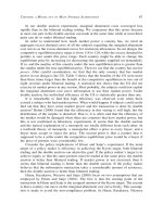
Each StarCatcher period lasts 240 seconds. At each instant, any idle player can
initiate a service request by clicking the Download button, as in Figure 1. The
service delay, or latency λ , is determined by an algorithm sketched in the paragraph
after next. Unless the download is stopped earlier, after λ seconds the player’s
screen flashes a gold star and awards her 10 points. However, each second of delay
costs the player 2 points, so she loses money on download requests with latencies
greater than 5 seconds. The player can’t begin a second download while an earlier
request is still being processed but she can click the Stop button; to prevent excessive losses the computer automatically stops a request after 10 seconds. The player

can also click the Reload button, which is equivalent to Stop together with an
immediate new download request, and can toggle between manual mode (as just
described) and automatic mode (described below).
The player’s timing decision is aided by a real-time display showing the results
of all service requests terminating in the previous 10 seconds. The player sees the
mean latency as well as a latency histogram that includes Stop orders, as illustrated
in Figure 1.
The delay algorithm is a noisy version of a single server queue model known in
the literature as M/M/1. Basically, the latency λ is proportional to the reciprocal of
current idle capacity. For example, if capacity is 6 and there are currently 4 active
users, then the delay is proportional to 1/(6 − 4) = 1/2. In this example, 5 users would
double the delay and 6 users would make the delay arbitrarily long. As explained in
Appendix A, the actual latency experienced by a user is modified by a mean reverting noise factor, and is kept positive and finite by truncating at specific lower and
upper bounds.
The experiments include automated players (called robots or bots) as well as
humans. The basic algorithm for bots is: initiate a download whenever the mean
latency (shown on all players’ screens) is less than 5 seconds minus a tolerance,
i.e., whenever it seems sufficiently profitable. The tolerance averages 0.5 seconds,
corresponding to an intended minimum profit margin of 1 point per download.
Appendix A presents details of the algorithm. Human players in most sessions have
the option of “going on autopilot” using this algorithm, as indicated by the toggle
button in Figure 1 Go To Automatic / Go To Manual. Subjects are told,


86

Experimental Business Research Vol. II

Figure 1. User interface. The four decision buttons appear at the bottom of the screen; the
download button is faded because the player is currently waiting for his download request

to finish. The dark box on the thick horizontal bar just above the decision buttons indicates
an 8 second waiting time (hence a net loss) so far. The histogram above reports results of
download requests from all players terminating in the last 10 seconds. Here, one download
took 2 seconds, two took 3 seconds, one took 5 seconds and one took 9 seconds. The color
of the histogram bar indicates whether the net payoff from the download was positive
(green, here light grey) or negative (red, here dark grey). The thin vertical line indicates
the mean delay, here about 3.7 seconds. Time remaining is shown in a separate window.


INTERNET CONGESTION
T

87

When you click GO TO AUTOMATIC a computer algorithm decides for you
when to download. There sometimes are computer players (in addition to your
fellow humans) who are always in AUTOMATIC. The algorithm mainly looks
at the level of recent congestion and downloads when it is not too large.
The network capacity and the persistence and amplitude of the background noise
is controlled at different levels in different periods. The number of human players
and bots also varies; the humans who are sidelined from StarCatcher for a few
periods use the time to play an individual choice game such as TreasureHunt,
described in Friedman et al. (2003). Table 1 summarizes the values of the control
variables used in all sessions analyzed below.
3. THEORETICAL PREDICTIONS
A player’s objective each period is to maximize profit Π = rN − cL, where r is the
reward per successful download, N is the number of successful downloads, c is the
delay cost per second, and L is the total latency time summed over all download
attempts in that period. The relevant constraints include the total time T in the
period, and the network capacity C. The constant of proportionality for latency, i.e.,

the time scale S, is never varied in our experiments.
An important benchmark is social value V*, the maximized sum of players’
profits. That is, V* is the maximum total profit obtainable by an omniscient planner
who controls players’ actions. Appendix A shows that, ignoring random noise, that
benchmark is given by the expression V* = 0.25S −1 Tr(1 + C − cS/r)2. Typical
S
parameter values in the experiment are T = 120 seconds, C = 6 users, S = 8 user-sec,
c = 2 points/sec and r = 10 points. The corresponding social optimum values are
U* = 2.70 active users, λ* = 1.86 seconds average latency, π * = 6.28 points per
download, N* = 174.2 downloads, and V* = 1094 points per period.
Of course, a typical player tries to increase his own profit, not social value. A
selfish and myopic player will attempt to download whenever the incremental
apparent profit π is sufficiently positive, i.e., whenever the reward r = 10 points
sufficiently exceeds the cost λ c at the currently displayed average latency λ. Thus
such a player will choose a latency threshold ε and follow
Rule R.

If idle, initiate a download whenever λ ≤ r/c − ε.
r

In Nash equilibrium (NE) the result typically will be inefficient congestion,
because an individual player will not recognize the social cost (longer latency times
for everyone else) when choosing to initiate a download. Our game has many pure
strategy NE due to the numerous player permutations that yield the same overall
outcome, and due to integer constraints on the number of downloads. Fortunately,
the NE are clustered and produce outcomes in a limited range.
E
To compute the range of total NE total profit V NE for our experiment, assume that
all players use the threshold ε = 0 and assume again that noise is negligible. No

31

27

10/2/03

10/3/03

164

112

164

194

214

143

104

216

155

127

193

199

243

192

189

159

Total
3

87

86

63

89

100

119

71

52

120

77

54

99

101

130

97

94

72

78

49

75

94

95

72

52

96

78

73

94

98

113

95

95

20

17

76

0

19

0

0

10

0

20

0

20

20

0

21

19

101

45

22

94

123

54

36

64

54

105

37

121

126

56

117

120

38

50

6

64

52

72

47

30

72

30

40

52

53

90

54

50

8

8

6

0

0

0

0

0

0

0

0

0

0

0

0

0

5

4

high

low
2

By capacity

By volatility

# of player-periods

0

0

0

0

88

60

0

90

0

50

0

0

97

0

0

0

6

20

0

0

0

0

0

0

0

0

0

0

0

0

0

0

0

7

Volatility: low: Sigma = .0015, Tau = .0002; Volatility: high: Sigma = .0025, Tau = .00002

31

27

2/19/03

5/23/03

18

27

2/12/03

2/14/03

27

16

2/5/03

2/4/03

16

24

32

1/24/03

32

9/12/02

9/5/02

1/31/03

32

32

8/20/02

9/11/02

27

32

8/21/02

# of
periods

8/22/02

Date

Table 1. Design of Sessions

24

0

0

0

0

0

0

0

0

0

0

0

0

0

0

0

9

6

4

5

4

4

4

4

4

4

4

4

5

0

4

4

4

Max
# of
robots

6

4

6

4

6

6

4

6

4

6

4

3

6

4

4

4

Max #
human
players

no

no

no

yes

no

no

no

yes

no

no

no

yes

yes

yes

no

no

Experienced
humans

88
Experimental Business Research Vol. II


INTERNET CONGESTION
T

89

player will earn negative profits in NE, since the option is always available to remain
idle and earn zero profit. Hence the lower bound on V NE is zero. Appendix A derives
the upper bound V MNE = T(rC − cS)/S from the observation that it should never be
T
S
possible for another player to enter and earn positive profits. Hence the maximum

E
E
NE efficiency is V MNE/ V* = 4(C − cS/r)/ (1 + C − cS/r)2 = 4U MNE/(1 + U MNE )2. For the
parameter values used above (T = 120, C = 6, S = 8, c = 2 and r = 10), the upper
bound NE values are U MNE = 4.4 active users (players), λMNE = 3.08 seconds delay,
π MNE = 3.85 points per download, N MNE = 171.6 downloads, and V MNE = 660.1 points
per period, for a maximum efficiency of 60.4%.
The preceding calculations assume that the number of players m in the game is at
least U MNE + 1, so that congestion can drive profit to zero. If there are fewer players,
t
then in Nash equilibrium everyone is always downloading. In this case there is
excess capacity a = U MNE + 1 − m = C + 1 − cS/r − m > 0 and, as shown in the
Appendix, the interval of NE total profit shrinks to a single point, Πm = Tram/S.
What happens if the background noise is not negligible? As explained in the
Appendix, the noise is mean-reverting in continuous time. Thus there will be some
good times when effective capacity is above C and some bad times when it is lower.
E
Since the functions V MNE and V* are convex in C (and bounded below by zero),
Jensen’s inequality tells us that the loss of profit in bad times does not fully offset
the gain in good times. When C and m are sufficiently large (namely, m > C > cS/r
+ 1, where the last expression is 2.6 for the parameters above), this effect is stronger
E
V
for V* than for V MNE. In this case Nash equilibrium efficiency V MNE/ V* decreases
when there is more noise. Thus the prediction is that aggregate profit should increase
but that efficiency should decrease in the noise amplitude σ / 2τ (see Appendix A).1
A key testable prediction arises directly from the Nash equilibrium benchmarks.
The null hypothesis, call it full rent dissipation, is that players’ total profits will be in
the Nash equilibrium range. That is, when noise amplitude is small, aggregate profits
S

will be V MNE = Tram/S in periods with excess capacity a > 0, and will be between 0
and V MNE = T(rC − cS)/S in periods with no excess capacity. The corresponding
T
S
expressions for efficiency have already been noted.
One can find theoretical support for alternative hypotheses on both sides of the
null. Underdissipation refers to aggregate profits higher than in any Nash equilibrium, i.e., above V MNE. This would arise if players can maintain positive thresholds
ε in Rule R, for example. A libertarian justification for the underdissipation hypothesis is that players somehow self-organize to partially internalize the congestion
externality (see e.g., Gardner, Ostrom, and Walker, 1992). For example, players
may discipline each other using punishment strategies. Presumably the higher profits
would emerge in later periods as self-organization matures. An alternative justification
from behavioral economics is that players have positive regard for the other players’
utility of payoffs, and will restrain themselves from going after the last penny of
personal profits in order to reduce congestion. One might expect this effect to weaken
a bit in later periods.
Overdissipation of rent, i.e., negative aggregate profits, is the other possibility.
One theoretical justification is that players respond to relative payoff and see increasing


90

Experimental Business Research Vol. II

returns to downloading activity (e.g., Hehenkamp et al., 2001). A behavioral economics justification is that people become angry at the greed of other players and
are willing to pay the personal cost of punishing them by deliberately increasing
congestion (e.g., Cox and Friedman, 2002). Behavioral noise is a third possible
justification. For example, Anderson, Goeree and Holt (1998) use quantal response
equilibrium, in essence Nash equilibrium with behavioral noise, to explain overdissipation in all-pay auctions.
Further insights may be gained from examining individual decisions. The natural
null hypothesis is that human players follow Rule R with idiosyncratic values of the

threshold ε . According to this hypothesis, the only significant explanatory variable
for the download decision will be λ − r/c = λ − 5 sec, where λ is the average latency
r
currently displayed on the screen. An alternative hypothesis (which occurred to us
only after looking at the data) is that some humans best-respond to Rule R behavior,
by anticipating when such behavior will increase or decrease λ and reacting to the
anticipation.
The experiment originally was motivated by questions concerning the efficiency
impact of automated Rule R strategies. The presumption is that bots (and human
players in auto mode) will earn higher profits than humans in manual mode.2 How
strong is this effect? On the other hand, does a greater prevalence of bots depress
everyone’s profit? If so, is the second effect stronger than the first, i.e., are individual
profits lower when everyone is in auto mode than when everyone is in manual
mode? The simulations reported in Maurer and Huberman (2001) confirm the
second effect but disconfirm the social dilemma embodied in the last question. Our
experiment examines whether human subjects produce similar results.
4. RESULTS
We begin with a qualitative overview of the data. Figure 2 below shows behavior in
a fairly typical period. It is not hard to confirm that bots indeed follow the variable
λ = average delay: their download requests cease when λ rises above 4 or 5, and the
line indicating the number of bots downloading stops rising. It begins to decline as
existing downloads are completed. Likewise, when λ falls below 4 or 5, the number
of bot downloads starts to rise.
The striking feature about Figure 2 is that the humans are different. They appear
to respond as much to the change in average delay. Sharp decreases in average delay
encourage humans to download. Perhaps they anticipate further decreases, which
would indeed be likely if most players use Rule R. We shall soon check this conjecture more systematically.
Figure 3 shows another surprise, strong overdissipation. Both bots and humans
lose money overall, especially bots (which include humans in the auto mode). The
top half of human players spend only 1% of their time in auto mode, and even the

bottom half spend only 5% of their time in auto mode. In manual mode, bottom half
human players lose lots of money but at only 1/3 the rate of bots, and top half
humans actually make modestly positive profit.


INTERNET CONGESTION
T

91
Tau: 0.0002
Sigma: 0.0015
Scale: 8000

12

# of humans: 3
# of robots: 4
Capacity: 3

10
8
6
4
2
0
−2
Avg. delay
# of humans downloading

−4

Delay change in last 2s
# of robots downloading

Figure 2. Exp. 09-12-2002, Period 1.
0.2
0.1

0.1
0
−0.04

−0.1
−0.2

1%

−0.3
−0.4

Time in
auto mode

−0.19
5%

−0.36

−0.5
−0.53

−0.6
−0.63

−0.7
Humans & robots

Top half of humans
Auto mode

Bottom half of humans

Manual mode

Figure 3. Profit per second in auto and manual mode.

Figure 4 offers a more detailed breakdown. When capacity is small, there is only
a small gap between social optimum and the upper bound aggregate profit consistent with Nash Equilibrium, so Nash efficiency is high as shown in the green bars
for C = 2, 3, 4. Bots lose money rapidly in this setting because congestion sets in


92

Experimental Business Research Vol. II

Points (% of social optimum)

1
0.5
0

−0.5
−1
−1.5
−2
−2.5
−3
−3.5
2

3

4

max NE
Actual (exper. humans)

5
Capacity (C)

6

7

9

Actual (humans and robots)
Actual (inexper. humans)

Figure 4. Theoretical and actual profits as percentage of social optimum.

quickly when capacity is small. Humans lose money when inexperienced. Experienced human players seem to avoid auto mode and learn to anticipate the congestion
sufficiently to make positive profits. When capacity is higher (C = 6), bots do
better even than experienced humans, perhaps because they are better at exploiting
the good times with excess capacity. (Of course, overdissipation is not feasible with
excess capacity: in NE everyone downloads as often as physically possible and
everyone earns positive profit.)
We now turn to more systematic tests of hypotheses. Table 2 below reports OLS
regression results for profit rates (net payoff per second) earned by four types of
players. The first column shows that bots (lumped together with human players in
auto mode) do much better with larger capacity and with higher noise amplitude,
consistent with NE predictions. The effects are highly significant, statistically as
well as economically. The other columns indicate that humans in manual mode are
able to exploit increases in capacity only about half as much as bots, although the
effect is still statistically highly significant for all humans and top half of humans.
The next row suggests that bots but not humans are able to exploit higher amplitude
noise. The last row of coefficient estimates finds that, in our mixed bot-human
experiments, the interaction [noise amplitude with excess fraction of players in auto
mode] has the opposite effect for bots as in Maurer and Huberman (2001), and has
no significant effect for humans.
Table 3 above reports a fine-grained analysis of download decisions, the dependent variable in the logit regressions. Consistent with Rule R (hardwired into their
algorithm), the bots respond strongly and negatively to the average delay observed
on the screen minus r/c = 5. Surprisingly, the regression also indicates that bots are
more likely to download when the observed delay increased over the last 2 seconds;
we interpret this as an artifact of the cyclical congestion patterns. Fortunately