MONEY, MACROECONOMICS AND KEYNES phần 8 doc

Second, the aggregate demand function is assumed to be less sensitive to the
interest rate than is aggregate supply, and hence the AD schedule cuts the AS from
above. The relative insensitivity of aggregate demand to interest rate changes was,
of course, a staple of the ‘Old Keynesian’ literature (and was implicit in the
Keynesian Cross). However, in that context it was not combined with a palpable
degree of interest sensitivity of supply, as is done here. For simplicity, the AD
schedule in Fig. 15.2 is shown as completely interest insensitive. However, clearly
nothing would be changed by allowing some interest elasticity, as long as this is
less than on the supply side.
The third important point is that in Fig. 15.2 the (real) rate of interest is taken
to be a financial variable determined essentially by the monetary policy of the
central bank. It is determined outside the aggregate demand and supply nexus
itself, and in the diagram shows up as a horizontal line across the page, at a pre-
determined level, . The underlying monetary theory is therefore that of the Post
Keynesian ‘horizontalist’ school, in which the interest rate (including the real
rate) is effectively a policy instrument, and the money supply is endogenous. This
is contrasted with Barro’s version in Fig. 15.1, in which there in no theory of
money and the interest rate is taken literally to be a real (non-monetary) variable.
Victoria Chick (e.g. 1984, 1986, 1991, 1995) has written extensively on Post
Keynesian monetary theory, endogenous money, the theory of banking and
alternative views on interest rate determination. She has indeed described hori-
zontalism (e.g. that of Moore 1979)
4
as an ‘extreme’ position (Chick 1986: 116),
while nonetheless making it clear that as a first approximation this is still a far
more reasonable assumption than the alternative (neoclassical) extreme. The main
objection to treating the interest rate as a purely policy-determined variable would
be the extent to which this neglects Keynes’s insights about liquidity preference
and the role of speculation in financial markets (Chick 1995: 31). The practical
implication would be that there can be occasions in which the monetary authori-
ties may not get their way in setting the interest rate.

5
Keynes himself had argued
this way in the General Theory (Keynes 1936: 202–4), although elsewhere (even
as late as 1945) he had stated that ‘The monetary authorities can have any inter-
est rate they like …Historically …(they) …have always determined the rate at
their own sweet will…’ (as quoted by Moore 1988b: 128).
For our present purposes, however, the debate about the precise degree of con-
trol of interest rates by central bankers may perhaps be set on one side. There
would clearly be general agreement that the stance of monetary policy is at least
a major influence on the real interest rate. Moreover, from the perspective of the
principle of effective demand, the main point at issue is not exactly how the rate
is set, but rather that it is not taken to be determined by demand and supply in
barter capital markets, as in the neoclassical model, and is exogenous to the ‘real
economy’ in that sense.
6
Note, however, that if we do proceed to take the interest rate as either an exoge-
nous or directly policy-determined variable, the issue immediately arises as to
how demand and supply could ever come into equilibrium. In neoclassical or new
rЈ
J. SMITHIN
154
classical theory, interest rate adjustment itself is supposed to be the equilibrating
mechanism, but that is ruled out in any horizontalist approach. However, it can be
suggested here that for the SOE an obvious equilibrating mechanism does exist,
namely changes in the real exchange rate. Or, it would be more accurate to say, a
combination of real exchange rate changes and output adjustment. This issue is
taken up below.
4. A simple aggregate demand and supply model for
the small open economy
Consider the following simple aggregate demand and supply ‘curves’ (they are

actually linear) for the SOE:
, (1)
. (2)
Equation (1) represents the aggregate demand schedule. The demand for output
depends positively on autonomous spending, A(t), as in traditional Keynesian
models, and positively on Q(t), where Q(t) is the real exchange rate. The nominal
rate is defined as the domestic currency price of one unit of foreign exchange, so
an increase in Q(t) represents a real depreciation. The argument is therefore that
a real depreciation increases the demand for net exports and hence total aggregate
demand. As discussed, for the sake of argument there is assumed to be no inter-
est rate term in eqn (1), which is an extreme instance of the view that the demand
schedule is insensitive to interest rate changes.
Equation (2) is the aggregate supply schedule. This is assumed to be negatively
sloped, not positively sloped, for the reasons discussed above. Also, a real depre-
ciation is taken to have a negative impact on supply. This arises as the result of
real wage resistance on the part of the labour force, and/or because of an increase
in the real costs of imported raw materials.
We can rearrange eqn (1) to yield
. (3)
Then use (3) in (2) and set aggregate demand equal to aggregate supply:
(4)
Now solve for Y(t):
(5)ϩ
{
␣(1)␤(2)/[␣(2)

ϩ

␤(2)]
}

A(t)

Ϫ

{
␣(2)␤(1)/[␣(2)

ϩ

␤(2)]
}
r(t)
Y(t)

ϭ

[␣(0)␤(2)

ϩ

␣(2)␤(0)]/[␣(2)

ϩ

␤(2)]
ϩ
{
[␣(1)␤(2)]/␣(2)
}
A(t).

Y(t)

ϭ

␤(0)

Ϫ

␤(1)r(t)

Ϫ

[␤(2)/␣(2)]Y(t)

ϩ

[␣(0)␤(2)]/␣(2)
Q(t)

ϭ

Y

d
(t)/␣(2)

Ϫ

␣(0)/␣(2)

Ϫ

[␣(1)/␣(2)]

A(t)
Y

s
(t)

ϭ

␤(0)

Ϫ

␤(1)r(t)

Ϫ

␤(2)Q(t)
Y

d
(t)

ϭ

␣(0)

ϩ

␣(1)A(t)

ϩ

␣(2)Q(t)
AGGREGATE DEMAND
155
It is immediately apparent that eqn (5) yields very ‘Keynesian’ results on the
determination of output and employment, meaning literally by this the kind of pol-
icy views that J. M. Keynes put forward at various points during his career.
Specifically, an increase in effective demand will permanently increase the level of
output, as will a cheap money policy in the sense of lower real rates of interest.
The real exchange rate is also an endogenous variable in the SOE context.
From eqns (1) and (2) we obtain
.
(6)
Then solving for Q(t):
(7)
According to eqn (7) a cheap money policy will cause a real depreciation. On the
other hand, a demand expansion actually seems to cause a real appreciation. This
latter result is consistent with Mundell–Fleming type models of the SOE,
although in this case the logic is not confined only to the short-run. However, it
should also be pointed out that the result seems to negate traditional concerns
about how a Keynesian-type demand expansion impacts the balance of payments.
For example, Smithin and Wolf (1993), and Smithin (2001), argue that a demand
expansion will lead to a real depreciation, but (in effect) that this should be toler-
ated as the expansion will also increase output and employment. In the present
framework, however, an increase in effective demand causes both an increase in

output and a real appreciation, so that this implicit trade-off is not a problem. This
is clearly an issue requiring further detailed research.
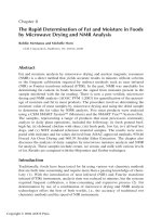
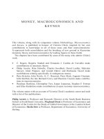
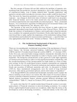
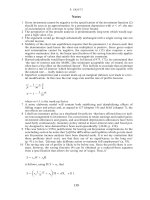
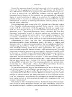
Figures 15.3 and 15.4 provide further intuition on the impact of lower interest
rates and a demand expansion, respectively.
Figure 15.3 illustrates the adjustment to a lower real rate of interest. The lower
interest rate increases aggregate supply along the AS curve, but at the same
time causes a real depreciation of the exchange rate. This has two effects: first a
reduction in aggregate supply (a leftward shift of the AS curve), and also an
increase in aggregate demand because of the stimulative effect on net exports. The
net impact (at point b) is higher output and employment, and a permanent real
depreciation.
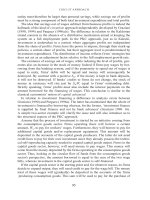
Figure 15.4 shows that an increase in effective demand also causes an increase
in output and employment. An increase in autonomous expenditures causes a
rightward shift of the AD schedule, but also a real appreciation of the exchange
rate. This then offsets the initial increase in demand to some extent, but also
causes an outward shift in supply. The final effect (at point b) is an overall
increase in output and employment. In this sense, the principle of effective
demand is reinstated.
Ϫ
{
␤(1)/␣(2)

ϩ

␤(2)]
}
r(t).
Q(t)

ϭ

[␤(0)

Ϫ

␣(0)]/[␣(2)

ϩ

␤(2)]

Ϫ

{
␣(1)/[␣(2)

ϩ

␤(2)]}

A(t)
␣(0)

ϩ

␣(1)A(t)

ϩ

␣(2)Q(t)

ϭ

␤(0)

Ϫ

␤(1)r(t)

Ϫ

␤(2)Q(t)
J. SMITHIN
156
5. Demand and supply constraints in currency unions
An interesting application of the above analysis is to the case mentioned in the
introduction where an SOE which is a member of a currency union is deprived of
the adjustment mechanism via real exchange rates. The obvious point to be made in
these circumstances is that monetary (interest rate) policy is now the prerogative of
the union-wide central bank rather than the individual national central banks.
Presumably, the analysis of relations with the rest of the world, outside the
union, would be similar to that illustrated in Fig. 15.3 above. A tight money (high
AGGREGATE DEMAND
157
Y
AS
AD
0
r
1

r
2
r
a
b
Figure 15.3 Adjustment to a lower real rate of interest
0
r
1
r
AD
AS
ADЈ
Y
a
b
Figure 15.4 Effect of a change in demand on output and employment
interest rate) policy would tend to reduce output and employment, but cause a real
appreciation of the external exchange rate. Similarly, a cheap money policy would
tend to increase output and employment, and depreciate the external exchange
rate. In the actual case of the contemporary Euro-zone, however, given the trade
diversion activities of the last several decades leading up to the establishment of
the single currency, there may be some reason to doubt how much benefit the
region as a whole would actually obtain from a depreciation.
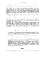
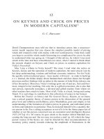
The impact of cheap money on the individual member-state, meanwhile, is
illustrated in Fig. 15.5.
Figure 15.5 suggests that the domestic economy which is embedded in the cur-
rency union may be supply constrained at the relatively high real rates of interest,
but then demand constrained at lower real interest rates. By hypothesis we have
eliminated the mechanism by which demand and supply were previously brought

into equilibrium, and, at least in the present simple example, have not suggested
any other. This does not a priori rule out the possibility that some alternative
equilibrating mechanism might eventually be discovered, but it does place the
onus on the supporters of these currency arrangements to give some hint as to
what this might be.
7
If no equilibrating mechanism can be found, the following result seems to
apply. A cheap money policy by the union-wide central bank, assuming that they
can be persuaded to take such action, would succeed in increasing output and
reducing unemployment up to a point. However, once real interest rates are
already ‘low’, any further increases in output would need to come about by
demand expansion (such as an expansionary fiscal policy by the domestic gov-
ernment). In light of the model presented here, an interesting ‘catch 22’ of the
practical situation in the contemporary EU is that this is explicitly ruled out for
J. SMITHIN
158
AD
AS
r
r 1
r 2
r 3
r 4
Y
0
Figure 15.5 Impact of cheap money on the individual member-state
the formerly sovereign national governments by the Pact for Stability and Growth.
Comparing Fig. 15.5 with Figs 15.3 and 15.4, it therefore seems that there is a
range of output levels which would formerly have been attainable given certain
policy choices under the old currency arrangements, but which are now no longer

attainable.
6. Capital flows and the potential for interest rate autonomy for
the small open economy
A gap in the argument of the present chapter is that it has not presented, even in
the benchmark flexible exchange rate case, a complete analysis of international
flows of funds and their impact on the interest rate and exchange rate changes
under discussion. A common counter-argument to the above would be that, under
modern conditions, and particularly as a result of greatly increased capital mobil-
ity, the contemporary SOE would not have a great deal of interest rate autonomy
even prior to accession to a monetary union. Hence, implicitly, the loss of the
ability to conduct monetary policy is not all that significant.
This argument has been dealt with in some detail, however, in earlier work by
(e.g.) Paraskevopoulos et al. (1996), Paschakis and Smithin (1998) and Smithin
(1999). In these contributions it is argued that even under modern conditions, the
SOE with a floating exchange rate may still have considerable interest rate auton-
omy, provided that the local authorities have the necessary political will. If so,
then the discussion (of monetary policy in particular) in the previous section
would retain some relevance.
The main point is that globalization, increased capital flows, and technical
change do move the world ever closer to the textbook case of perfect capital
mobility, but, as long as there are separate monetary systems and exchange rates
are free to change, this does not necesssarily imply that there will be perfect asset
substitutability. In other words a currency risk premium will continue to exist and
this can insert a wedge between domestic and foreign real interest rates, allowing
for some degree of domestic interest rate autonomy. Under certain conditions, as
discussed in the literature cited above, the domestic authorities may be able to
manipulate the risk premium in their favour.
Of course, any type of interest rate autonomy disappears entirely in the case of
fixed exchange rate regimes, currency boards and currency unions, and this may
be precisely why these arrangements are advocated in certain quarters. In any

event, these remarks do indicate the type of arguments that need to be made to
defend the foregoing analysis against some standard objections.
7. Conclusion
The policy lessons which might have been learnt from so-called ‘Keynesian eco-
nomics’ are the importance of (a) a high level of effective demand, and (b) low
real rates of interest, for the healthy functioning of a capitalist economy. However,
AGGREGATE DEMAND
159
Keynesian economics is now in eclipse and a main concern of orthodox or neo-
classical economics for the past thirty-five years has been to construct a theoretical
apparatus which denies these propositions and aggressively asserts the opposite.
Some part of this process has been illustrated by the discussion in this paper of the
evolution of aggregate demand and supply analysis in the economics textbooks.
Moreover, certain contemporary institutional changes, among them certainly
the European single currency project in the form shaped by the Treaty of
Maastricht and the Pact for Stability and Growth, actually seem to take the form
of imposing neoclassical scarcity economics by fiat (cf. Parguez 1999). The
sketch above of the supply and demand constrained SOE in a currency union pro-
vides at least a potential starting point for a more detailed examination of this
kind of issue.
Victoria Chick is, of course, a very distinguished academic economist who has
held out courageously against the anti-Keynesian tide in the academy in our
times, and in her writings has provided many of the necessary theoretical build-
ing blocks for a coherent alternative approach with which to ‘complete the
Keynesian revolution’ (Chick 1995: 20). The present contribution is offered in a
similar spirit.
Notes
1 The author would like to thank Sheila Dow, Markus Marterbauer, Hana Smithin, and
conference participants at the annual meetings of the Eastern Economic Association
(Washington DC, March 2000), for helpful comments and suggestions which have

improved this chapter.
2 Snowdon and Vane (1997: 18–20) also stress that the demand and supply schedules in
the real business cycle model are ‘long-run’ constructs (in the textbook sense of not
depending on such assumptions as sticky nominal wages, etc.), as opposed to orthodox
Keynesian or new Keynesian ‘short-run’ analysis. However, the analysis below shows
that Keynesian-type results, including the impact of demand on employment, do not
depend at all on the textbook assumptions.
3 See also the discussion by Palley (1996, chapter 5).
4 The expression itself appears in the title of Moore’s (1988a) subsequent book.
5 Particularly if we are thinking of the real rate and particularly in a downward direction.
On this point, see also the discussion in Smithin (2000) regarding recent Japanese
experience.
6 See Lavoie (1996) and Rochon (1999) for more detailed discussion of the debate
between Post Keynesian horizontalists and structuralists, from a horizontalist perspec-
tive. Dow (1996) provides a critique of horizontalism. For Victoria Chick’s current read-
ing of the debate, see Chick (2000).
7 In the endogenous money setting, it is clearly impossible to appeal to real balance effects
and the like.
References
Barro, R. J. (1984). Macroeconomics. New York: John Wiley.
Burstein, M. L. (1995). Classical Macroeconomics for the Next Century. Toronto: York
University.
J. SMITHIN
160
Chick, V. (1983). Macroeconomics after Keynes. Cambridge, Massachusetts: MIT Press.
Chick, V. (1984). ‘Monetary Increases and their Consequences: Streams, Backwaters and
Floods’, in A. Ingham and A. Ulph (eds), Demand, Equilibrium and Trade: Essays in
Honour of Ivor F. Pearce. London: Macmillan, pp. 237–50.
Chick, V. (1986). ‘The Evolution of the Banking System and the Theory of Saving,
Investment and Interest’, Economies et Societies, 20(3), 111–26.

Chick, V. (1991). ‘Hicks and Keynes on Liquidity Preference: A Methodological
Approach’, Review of Political Economy, 3(3), 309–19.
Chick, V. (1995). ‘Is there a Case for Post Keynesian Economics?’, Scottish Journal of
Political Economy, 42(1), 20–36.
Chick, V. (2000). ‘Money and Effective Demand’, in J. Smithin (ed.), What is Money?
London: Routledge, 124–38.
Davidson, P. (1994). Post Keynesian Macroeconomic Theory. Aldershot: Edward Elgar.
Chick, V. and Smolensky, E. (1964). Aggregate Supply and Demand Analysis. New York:
Harper and Row.
Dornbusch, R. and Fischer, S. (1978). Macroeconomics. New York: McGraw-Hill.
Dow, S. C. (1996). ‘Horizontalism: A Critique’, Cambridge Journal of Economics, 20,
497–508.
Hicks, J. R. (1937). ‘Mr Keynes and the Classics’, Econometrica, 5, 144–59.
Keynes, J. M. (1936). The General Theory of Employment Interest and Money. London:
Macmillan.
Lavoie, M. (1996). ‘The Endogenous Supply of Credit-Money, Liquidity Preference and
the Principle of Increasing Risk: Horizontalism versus the Loanable Funds Approach’,
Scottish Journal of Political Economy, 43(3), 275–300.
MacKinnon, K. T. and Smithin, J. (1993). ‘An Interest Rate Peg, Inflation and Output’,
Journal of Macroeconomics, 15(4), 769–85.
Moore, B. J. (1979). ‘The Endogenous Money Stock’, Journal of Post Keynesian
Economics, 1(2), 49–70.
Moore, B. J. (1988a). Horizontalists and Verticalists. Cambridge: Cambridge University
Press.
Moore, B. J. (1988b). ‘Keynes’s Treatment of Interest’, in J. Smithin and O. F. Hamouda
(eds), Keynes and Public Policy after Fifty Years, Vol. 2, Theories and Method.
Aldershot: Edward Elgar, pp. 121–9.
Palley, T. I. (1996). Post Keynesian Economics. London: Macmillan.
Paraskevopoulos, C. C., Paschakis, J. and Smithin, J. (1996). ‘Is Monetary Sovereignty an
Option for the Small Open Economy?’, North American Journal of Economics and

Finance, 7(1), 5–18.
Parguez, A. (1999). ‘The Expected Failure of the European Economic and Monetary
Union: A False Money against the Real Economy’, Eastern Economic Journal, 25(1),
63–76.
Paschakis, J. and Smithin, J. (1998). ‘Exchange Risk and the Supply-Side Effect of Real
Interest Rate Changes’, Journal of Macroeconomics, 20(4), 703–20.
Rochon, L P. (1999). Credit, Money and Production: An Alternative Post Keynesian
Approach. Cheltenham: Edward Elgar.
Samuelson, P. A. and Scott, A. (1966). Economics (Canadian Edition). Toronto: McGraw-
Hill Company of Canada.
Smithin, J. (1986). ‘The Length of the Production Period and Effective Stabilization
Policy’, Journal of Macroeconomics, 8(1), 55–62.
AGGREGATE DEMAND
161
Smithin, J. (1997). ‘An Alternative Monetary Model of Inflation and Growth’, Review of
Political Economy, 9(4), 395–409.
Smithin, J. (1999). ‘Money and National Sovereignty in the Global Economy’, Eastern
Economic Journal, 25(1), 49–61.
Smithin, J. (2000). ‘Macroeconomic Policy for a Post-conservative Era: Can and Should
Demand Management Policies be Resuscitated?’, in H. Bougrine (ed.), The Economics
of Public Spending, Debt, Deficits and Economic Performance. Cheltenham: Edward
Elgar, pp. 57–77.
Smithin, J. (2000). ‘Monetary autonomy and financial integration’, in L P. Rochon and
M. Vernengo (eds), Credit, Effective Demand and the Open Economy: Essays in the
Horizontalist Tradition, Cheltenham: Edward Elgar, pp. 243–55.
Smithin, J. and Wolf, B. M. (1993). ‘What would be a “Keynesian” Approach to Currency
and Exchange Rate Issues?’, Review of Political Economy, 5(3), 365–83.
Snowdon, B. and Vane, H. R. (1997). ‘To Stabilize or not Stabilize: Is that the Question?’,
in Snowdon, B. and Vane, H. R. (eds), Reflections on the Development of Modern
Macroeconomics. Cheltenham: Edward Elgar, pp. 1–30.

J. SMITHIN
162
16
SOME MYTHS ABOUT PHILLIPS’S
CURVE
1
Bernard Corry
Some economists have had theorems, models, a statistic or statistical plot or
something or other named after them. To take a few examples, listed alphabeti-
cally to avoid any suggestion of ranking them, we have Arrow’s impossibility
theorem, the Cournot point, Gibrat distributions, the Harrod–Domar growth
model, Lorenz curves, the Lucas critique, the Modigliani–Miller theorem, Nash
equilibrium, Pareto optimality, the Samuelson–Stolper theorem, Solow’s growth
model, Tobin’s ‘q’, Walrasian equilibrium, and so on. But today I think it is fair
to say that among the better, if not best known, is the Phillips curve.
2
Any student
that has taken a basic economics course will have heard (even read!) a reference
to that curve. Yet there are numerous accounts of, among other things, what it
means, where it comes from, what theoretical and or statistical support it has, the
policy implications of it, and yet more.
In my contribution to this volume honouring Victoria Chick, I want to look at
what I call ‘myths’ about the Phillips curve. Vicky herself has been one of those
instrumental in trying to separate out the ‘myths’ surrounding Keynes’s econom-
ics from what goes under the heading ‘Keynesian’ in the popular economics lit-
erature (Chick 1983). Here I wish to make a contribution to the economics of
A. W. Phillips versus the literature (‘myths’) labelled ‘the Phillips curve’. I want
to contrast what Bill Phillips actually did in his famous paper – what I shall call
Phillips’s curve – from what has grown up to be ‘the Phillips curve’. I also want
to emphasise the point made by scholars of Phillips’s work that his famous curve

was not at all his important contribution to economic inquiry.
3
Does it matter that
the myths remain with us for students to pick up from popular textbooks, read by
millions, rather than get the truth from esoteric journals and monographs read by
hundreds? Well perhaps it does not.
4
Does it make us worse economists by believ-
ing in these myths? No, probably not, but I think we do owe a duty to the past con-
tributors to our discipline to ‘get the record straight’ where this is possible. And
indeed it may sometimes be the case that the original version offers much more
insight into the actual working of the real world than the modified versions that
have usurped the originals.
163
Now what do I mean by myths? Not necessarily falsehoods, that is statements
that can be shown or ‘proved’(?) to be false, but allegations, rumours, memories
about an idea, or person, that are now stated but which may not represent ‘what
actually’ happened, or was meant, or what was actually said or intended by a cer-
tain individual or group. We all have experience of these myths; perhaps it is
inevitable and there is not much we can do about it. These myths arise for various
reasons. Sometimes there is little or no documentation from the past and memo-
ries of the participants have been used – and, as we all know, memory is very
rarely reliable evidence.
May I take a brief example from my own experience; reference is often made
in the literature to the seminar at LSE in the late 1950s and early 1960s which
went under the name MMT (methodology, measurement and testing). Several dif-
ferent accounts are given of its membership, its aims, its work, etc. – as a mem-
ber of that group I have to say that some of the accounts do not at all accord with
my memories of it. This does not mean that these accounts are incorrect. It may
be, and probably is, my memory that is at fault! Myths are also sometimes used

to bolster or attack a position in academic debate. When I was a student (in the
late 1940s and early 1950s) ‘Hayekian’, ‘Austrian’, ‘Classical’ were dirty words,
‘Keynesian’ of course was good. Today we have almost complete role reversal in
the use of these adjectives! Now in many cases the use of these adjectives had lit-
tle or nothing to do with the actual purveyors of these ideas. Of course scholars
who have researched these particular myths will know them for what they are –
at best half truths and at the limit downright falsehoods.
5
So what are the main myths about the Phillips curve that I want to look at in this
paper? I must emphasise that I am here going to contrast what Phillips set out to
do and did in his original paper with the spate of literature that is prepared to call
anything relating inflation and unemployment as ‘the Phillips curve’! One story –
what may be termed the ‘popularist’ version – goes as follows. Keynes wrote an
important book in the mid-1930s; it did, however, have several (fatal?) lacunae,
one of which was its assumption of a constant general level of prices or – equally
flawed – the assumption that prices were constant until full employment, after
which output was constant and prices rose proportionally to money national
income. So there was no period when output and prices were rising together.
Therefore, ‘full employment’ policy was comparatively easy. Output had to be
expanded via demand management to the point where prices were just about to
rise. Economics had given the world the gift of full employment without inflation.
The Phillips curve filled this gap in Keynes’s analysis and demonstrated that
there was a negative non-linear trade-off between unemployment (as a proxy
for real output changes) and inflation. Albert Rees (1970: 227) put this point of
view as follows. ‘A major reason for the importance of Professor A. W. Phillips’
article … is that it seems to offer the policy maker a menu of choices between
employment and inflation’.
6
With the aid of social indifference curves showing
the subjective trade-off between inflation and unemployment, countries could

achieve a social optimum by finding the tangency point between the social
B. CORRY
164
indifference curve and the ‘objective’ Phillips curve. Further improvement could
be obtained by measures to shift or twist the Phillips curve. In such a world the
economist was God, and indeed it is probably true to say that in that era the pres-
tige of economists was as high as it has ever been. The arrival of stagflation in the
1960s put an end to all this trade-off nonsense! As a typical example, Matyas
(1985) writes of the impact of stagnation, ‘(t)his meant a complete bankruptcy of
the Phillips curve’ (p. 540). In any case researchers began to doubt whether the
Phillips, ‘trade-off’ curve had ever been there in the first place.
Another – and I believe more plausible – story goes as follows. Even in the
General Theory Keynes acknowledged the fact that there would be upward pres-
sure on prices as the economy approached full employment. UK – and USA –
wartime discussions of the possible postwar economic scene always voiced fears
that inflationary tendencies would be a major problem in a world committed to
high levels of employment. Full employment was thought to be at unemployment
rates of around 5 per cent. The actual postwar scene produced a much lower rate
of inflation and a lower level of unemployment than the pessimists had forecast.
However by the mid-1950s fears of inflationary pressures, and particularly the
likely effects on the balance of payments, were the subject of governmental and
academic debate.
7
There was a great deal of debate about the actual mechanics of
the inflationary process.
Now let us turn to Phillips and his curve; I shall develop my discussion in the
following manner. I begin with an historical reconstruction of the state of eco-
nomic debate when he did the work for his famous paper; I will then turn to
Phillips and his main contribution(s) to economic inquiry before I discuss the
Phillips curve itself. The questions ‘had it all been said before?’ and ‘was it an

attempt to fill a gap in Keynes?’, as well as ‘why was Phillips picked out?’, will
form the rest of the paper.
1. An historical reconstruction
By historical, as opposed to ‘rational’, reconstruction, I mean an attempt to look
at the actual problem situation as seen by the participants at the time rather than by
current investigators trying to work out what was in the minds of past researchers.
8
A central concern of macroeconomic debate in academic and political circles
in the mid-1950s, both in the UK and USA, was the cause(s) of inflation.
Although comparatively mild by later standards, the rate of inflation was begin-
ning to creep up and its interpretation revolved around what was commonly called
the competing hypotheses of ‘demand pull’ versus ‘cost push’. This debate tied in
with microeconomic discussions of price determination in individual markets and
the competing claims of market-forces versus cost-plus theories of price determi-
nation. So one had a permutation of commodity-market and factor-market deter-
mination along the lines of demand–demand; demand–cost; cost–demand;
cost–cost.
9
At the macro-level the main dispute ranged around the role of aggre-
gate demand flows versus trade union push in the inflationary sequence. This led
SOME MYTHS ABOUT PHILLIPS’S CURVE
165
to what may be termed the ‘spiral’ discussions and various permutations:
wage–price; price–wage; price–wage–price, etc! On the factor front the main
emphasis was on the role of wages in the inflationary process, although some
consideration was given to the role of import prices. The central issue was the
question of whether trades unions could exert an independent influence on prices
other than via changes in the demand for labour triggered by changes in aggre-
gate demand. So the relationship between aggregate demand and wage changes
was in the air!

Now if we recall Merton’s principle of multiple discovery, then it should not
surprise us that researchers widely scattered geographically and also in time
should come up with very similar pieces of research aimed at the same problem.
The history of economics is evidence of this principle. There is of course the
interesting question of why, out of the several similar contributions, it is usually
the case that one particular account should dominate the academic debate and
become known as ‘the’ contribution. Sometimes the answer lies in the personali-
ties of those who get the glory, those economists who are born conscious revolu-
tionaries – Smith, Ricardo, Marx, Jevons, Keynes, Friedman to name a few. They
contrast with the more evolutionary type of personality that emphasises the
continuity of their thinking rather than its ‘break with the past’. Mill (J. S.),
Edgeworth, Marshall, Pareto, Robertson, Stigler, Johnson, Tobin come to mind
here. Another reason why a particular contribution is singled out from its com-
petitors is that it is seen to have the clearest implications for policy and is easily
taken up by policy makers in the political arena. Undoubtedly Phillips’s curve was
helped on its way by Dick Lipsey’s follow-up paper (Lipsey 1960), but to my
mind the crucial push was provided by Samuelson and Solow in their famous
1960 paper. This was important for several reasons; two would suffice for our
purposes. The first is that it came from two very distinguished and respected
economists; secondly they switched the debate to the inflation–unemployment
trade-off – using incidentally for the first time the concept of a ‘menu’ of choice
between the two variables.
2. Phillips main contribution(s) to economics
Bill Phillips was trained as an electrical engineer and came to economics via his
degree at LSE where he studied for the B.Sc. (Economics) (1946–9). The title of
the degree was and is misleading. When he took the degree he specialised in soci-
ology and out of his nine finals papers would have had two in economics.
Textbooks available then were few. Cairncross (1944) and Benham (1938) led the
UK field to which was added those recent arrivals from the USA, Boulding
(1941) and Samuelson (1948). Phillips did once assert that his ideas for illustrat-

ing mechanisms for understanding and hopefully controlling economic systems
made famous in his Phillips machine construction – which owed a good deal
incidentally, as he acknowledged, to the economics input by Walter Newlyn –
stemmed from a diagram in Boulding linking stocks and flows in the elementary
B. CORRY
166
theory of price.
10
From his engineering studies he was familiar with feedback
mechanisms and the notion of optimal control.
Not long after graduating – in 1950 – he obtained an assistant lectureship in eco-
nomics at LSE and became a member of the LSE economics research division,
which was directed by Frank Paish. He then registered for a Ph.D. in economics
under the supervision of James Meade. His Ph.D., ‘On the Dynamics of Economic
Systems’, was successfully submitted in 1953, and a version of it was published in
1950 under the title ‘Mechanical Models in Economic Dynamics’ (Phillips 1950).
Phillips’s main concern and one that remained with him throughout his economic
studies was the problem of controlling economic systems when the basic structures
were not too clearly understood and where the estimation of these essentially
dynamic relationships posed enormous statistical difficulties. Hence for the fore-
seeable future for macroeconomic control the way ahead lay in automatic control
mechanisms using feedback rules. We may notice here the closeness of this
approach to Friedman’s ‘rules versus authority’ view of economic policy.
3. The content of Phillips’s curve
The research embodied in the 1958 paper was part of ongoing research into the
inflationary process in the UK being carried out at LSE. Frank Paish had developed
a view that wage increases were mainly explained by demand pressures and the best
way to measure these pressures was the gap between ‘full capacity’ output and
actual output. The explanatory variable was rather difficult to measure and Bill
Phillips looked for a more direct measure of the pressure of demand in the labour

market. To hand was a longish time series on unemployment that had been devel-
oped by Beveridge and a long series on wage rates then recently produced by Phelps
Brown and Hopkins. Thus Phillips used the percentage of the labour force unem-
ployed as his explanatory variable, his dependent variable being the percentage rate
of change of wage rates. He also acknowledged the need to allow for dynamic dis-
equilibrium so that for any given percentage unemployment rate, the effect on wage
rates would differ if unemployment were rising than if it were falling. So the rate of
change of unemployment was also an explanatory variable in his theoretical struc-
ture. He also included an allowance for cost influences on wages, which he thought
would mainly be captured by an index of import prices. But for his curve fitting of
wage rate changes against unemployment, Phillips did the following:
●
To eliminate the effect of the rate of change in unemployment he averaged
his data and eliminated the ‘loops’ of the raw data around his curve.
11
●
He surmised – on theoretical grounds – that the relationship would be non-
linear and thus rejected linear least squares regression in favour of ‘fitting by
eye’.
His fitted relationship was fairly good for some time periods he looked at, but
not for others. His own conclusion was that ‘the statistical evidence …seems in
SOME MYTHS ABOUT PHILLIPS’S CURVE
167
general to support the hypothesis that the rate of change of money wages can be
explained by the level of unemployment and the rate of change of unemployment,
except in or immediately after years in which there is a sufficiently rapid rise in
import prices to offset the tendency for increasing productivity to reduce the cost
of living’ (Phillips 1958 in Leeson 2000: 258–9). This is of course a long way
from a simple relationship between wage changes and unemployment, and miles
away from an inflation–unemployment trade-off!

4. Had it all been said before?
Among the main contenders that have been specifically mentioned in the litera-
ture are Irving Fisher, Arthur Brown and Paul Sultan. Let us take a brief look at
their work.
Irving Fisher’s paper is sometimes quoted as an early and more coherent trade-
off curve than Phillips. But on inspection the Fisher paper turns out to be a sta-
tistical plot of the relationship between price inflation and unemployment – not
Phillips’s curve – and it posits inflation as the independent variable. Of course the
effect of inflation on the level of economic activity – and hence on the level of
employment and unemployment – has a long history in economic thinking. There
was a particularly interesting controversy during and after the Napoleonic wars.
Arthur Brown’s work has a much greater claim to being a ‘forerunner’ of
Phillips’s curve as Thirlwall has cogently argued.
12
In chapter 4 of The Great
Inflation – published in 1955 but a long time in the writing – Brown considers the
‘nature and conditions of the Wage–Price Spiral’. He discusses the connection
between wage/price changes and employment – hence unemployment changes.
He argues that no efforts to date have been made to establish the connection
empirically nor to find the level of unemployment below which the wage–price
spiral comes into operation. Basically his mechanism is that demand changes –
measured by unemployment levels – feed into wage changes which then feed into
price changes. He also had the notion of loops and an expectational explanation
of them. ‘What would one expect to be the relation between the two variables dur-
ing a fluctuation of effective demand? In the recovery and boom effective demand
for labour is increasing, and, because it is expected to increase, it will be high rel-
atively to the existing level of activity and employment. Labour is becoming
scarcer, that …so its bargaining power is increasing, which will be likely to mean
that the rate at which it can raise wages is increasing.’ (Brown 1955: 91).
Brown (op. cit.) also considers trade union power and different types of unem-

ployment to account for rigidities in the rate of changes of wages in the downturn.
He plots unemployment against the rate of change of wages but does allow for the
influence of other variables and does not find any strong relationship.
Nonetheless Brown’s work is clearly along the lines of Phillips’s later paper. There
is no reference to Arthur Brown in the Phillips paper – in fact other than statisti-
cal sources there are no references quoted in the paper. But later on in his career
in a biographical note we do get an acknowledgement of A. J. Brown. Of his
B. CORRY
168
famous 1958 article Phillips wrote ‘[I]t was a rush job. I had to go off on sabbati-
cal leave to Melbourne; but in that case it was better for understanding to do it
simply and not wait too long. A. J. Brown had almost got these results earlier, but
failed to allow for the time lags.’ (Bergstrom et al. 1978: xvi).
Our third candidate for the originator of ‘Phillips’s Curve’ is Paul Sultan,
indeed in their piece championing his cause Amid-Hozour, Dick and Lucier sug-
gest the term ‘Sultan Schedule and Phillips Curve’ (Amid-Hozour et al. 1971:
319). But in his Labour Economics – on which the claim is based – we read the
following description of his diagram, ‘(t)he vertical scale measures the annual
change in the price level expressed as a percentage, while the horizontal scale
measures the percentage of the work force unemployed’ (Sultan 1957: 319).
As with Fisher, Sultan’s work is concerned with what I have called – following
accepted usage – ‘the Phillips Curve’, that is the relationship between the inflation
rate and the percentage of the labour force unemployed. This is not Phillips’s curve.
Indeed the lineage of direct discussion of the Phillips curve is a rather short
one. Discussions subsequent to Phillips’s paper were initially about the strength
and theoretical basis of the relationship between wage changes and unemploy-
ment. The famous Lipsey paper clearly added great momentum to this type of
research both in terms of the theoretical generating mechanism and the appropri-
ate estimation procedures. Attempts were made to unpack the theory and others
tried to find extra explanatory variables. For example Kaldor’s profits theory of

wage increases, or Hines’s trade union variable.
13
But soon the Phillips curve
became the ‘trade-off’ curve between inflation and unemployment and as we
stated earlier the coup de grace was (apparently) given to this by stagflation. As
usual, or at least as is often the case in economics, theoretical explanation rapidly
followed the uncomfortable new facts and explanation was soon at hand to
demonstrate that, if only we had understood rational expectations from the start,
we would not have expected to have found a Phillips curve in the first place! And
indeed earlier statistics that seemed to support the then maintained hypothesis are
shown (apparently!) to be suspect. The disappearing Phillips curve was never
there in the first place!
5. Filling a gap in Keynes?
It depends what you think the gap in Keynes was. I referred above to the ‘popu-
lar’ view that Keynes really had nothing to say about the price level and its rela-
tion to the overall state of the economy. This view is a travesty of Keynes! Keynes
never posited an inverted-L supply curve. The introduction into mainstream eco-
nomics of the fixed price world was a product of the interpreters of Keynes –
especially the ISLM analysis, and the so-called 45Њ approach. It did become a
stick with which to beat the ‘Keynesians’ and to demand theoretical changes to
modify ‘Keynesian’economics. But among followers of Keynes – Joan Robinson,
Meade and the like – an upswing was always going to drag along with it wages
and prices. The issues were what was the mechanism of causality, how rapidly
SOME MYTHS ABOUT PHILLIPS’S CURVE
169
would it occur and what to do about it. Unfortunately into the textbooks and
standard teaching of macroeconomics came ‘Keynesian’ economics with the
inevitable reaction.
6. Why was Phillips’s curve picked out?
14

We have already partially discussed this issue in our remarks above about why
certain ideas in economics are taken up rather than others. This is a complex issue
and we do not have space here to take up the question at great length. There are
many aspects to be considered and the reasons will vary from (were it true!) gen-
uine scientific advance to the politically driven. By the latter I mean that we
observe changes in political philosophy brought on for various reasons – one of
which may be a temporary breakdown of the economic machine – which gener-
ate a new set of economic orthodoxies. These new economic precepts may be
fished out from existing but temporarily discarded ideas or may be ‘new’. I have
previously argued this notion with respect to the natural rate hypothesis (Corry
1995). Now what about Phillips’s curve? It is certainly true that it hit the head-
lines rapidly. Basil Yamey – the then editor of Economica – has related how sales
of that journal leapt for that one issue (Yamey, in Leeson 2000).
It also gained by being a product of the LSE with its location in London and near
the media powerhouses. Those hankering after a planned economy with a key role
to government in the control of the economy saw in the Phillips curve a defence of
incomes policy, of productivity geared wage increases and even regional policy. But
it also gave ammunition to the free marketeers: unemployment became the key
weapon in the fight against inflation (shades of Marx!) and if that sounded too
harsh, then labour market flexibility was the order of the day (smash the unions!).
What is certain is that Bill Phillips himself would never have given so much
importance to his tentative empirical work. The real lesson that Bill Phillips
wanted economists to learn was the dangers inherent in the advocacy of economic
policies when the structure of the underlying economic system was not ade-
quately understood and was subject to unforeseen (unforeseeable?) changes in
that structure. The lesson is as usual ‘Be Critical’, ‘Be Humble’ and do not be
sweet-talked by politicians!
Notes
1 As I was near the completion of this article I received a copy of Robert Leeson’s mag-
nificent collection of articles by Bill Phillips and commentaries by recognised experts

on his work. The volume is a mine of information for all those interested in the work
and career of Bill Phillips.
2 Of course Bill Phillips has another memorial in the economists hall of fame, namely the
Phillips machine!
3 This point was made clear in the 1978 volume of essays in honour of the memory of
A. W. H. Phillips (Bergstrom et al. 1978) but is made even more forcibly in the recent
Leeson (ed) (2000) volume.
B. CORRY
170
4 But perhaps it does. Some of the central concerns expressed by Keynes about the work-
ing and potential instability of capitalism without careful regulation were lost to the
mainstream of the profession because of what may be termed ‘crude’Keynesianism by
which a bowdlerised account of his ideas entered basic economics teaching. Victoria
Chick has been at the forefront of those trying to correct these tendencies.
5 Even among scholars, and after long years of research and debate, the interpretation of
past writers and their ideas still can lead to profound disagreements and indeed ani-
mosity. Historians of economic thought will doubtless be familiar with the debate over
the ‘correct’interpretation of classical economics that goes on among such luminaries
as Hollander, Blaug, O’Brien, Peach and co.
6 This was not however the view that Albert Rees took.
7 For an excellent account of these debates, see Hutchison (1968, especially chapter 3).
8 Here I am in near agreement with Blaug’s (1999) remark that ‘I vote for historical
reconstructions as the only legitimate occupation of historians of economic thought’
(p. 214).
9 Here an important influence was Bent Hansen’s Study in the Theory of Inflation
(Hansen 1951).
10 On the Boulding influence, see Walter Newlyn’s contribution to the Leeson (2000)
volume.
11 This procedure led to the criticism put forward by Desai (1975) that Phillips’s curve
was a long-run equilibrium relationship that could not provide any policy conclusions

with respect to short-run movement along Phillips’s curves.
12 Indeed a case can be made for referring to Brown–Phillips curves.
13 For an excellent survey of the early follow-up work on Phillips’s curve, as opposed to
the Phillips curve see Peston (1971).
14 For a very astute analysis of this problem, see Sawyer (1987).
References
Amid-Hozour, E., Dick, D. T., Lucier, R. L. (1971). ‘Sultan Schedule and Phillips Curve;
An Historical Note’; Economica, 38, 319–20.
Benham F. C. (1938). Economics: A General Introduction. London: Pitman.
Bergstrom, A. R., Cutt, A. J. L., Peston, M. H. and Silverstone, B. D. J. (Eds) (1978).
Stability and Inflation: A Volume of Essays to Honour the Memory of A. W. H. Phillips.
Chichester: Wiley; for the New Zealand Association of Economists, Inc.
Blaug, M. (1999). ‘Misunderstanding Classical Economics: The Sraffian Interpretation of
the Surplus Approach’, History of Political Economy, 31, 213–36.
Boulding, K. E. (1941). Economic Analysis. Harper.
Brown, A. W. (1955). The Great Inflation 1939–1951. Oxford: Oxford University Press.
Cairncross, A. (1944). Introduction to Economics. London: Butterworths.
Chick, V. (1983). Macroeconomics after Keynes. Deddington: Philip Allan.
Corry, B. A. (1995). ‘Politics and the Natural Rate Hypothesis; A Historical Perspective’,
in R. D. Cross (ed.), The Natural Rate of Unemployment. Cambridge: Cambridge
University Press
Desai, M. (1975). ‘The Phillips Curve: A Revisionist Interpretation’, Economica, 42, 1–19.
Donner, A. and McCollum, J. F. (1972). ‘The Phillips Curve. An Historical Note’,
Economica, 39, 323–4.
Fisher, I. (1926). ‘A Statistical Relationship Between Unemployment and Price Changes’,
International Labour Review, June.
Hansen, B. (1951). Study in the Theory of Inflation. London: George Allen and Unwin.
SOME MYTHS ABOUT PHILLIPS’S CURVE
171
Hutchison, T. W. (1968), Economics and Economic Policy in Britain 1946–66. London:

George Allen and Unwin.
Johnson, H. G. and Nobay, A. R. (ed.) (1971). The Current Inflation. London: Macmillan.
Leeson, R. (ed.) (2000). A W H Phillips: Collected Works in Contemporary Perspective.
Cambridge: Cambridge University Press.
Lipsey, R. G. (1960). ‘The Relation between Unemployment and the Rate of Change of
Money Wage Rates in the United Kingdom, 1862–1957. A Further Analysis’,
Economica, 27, 1–31.
Lipsey, R. G. (2000). ‘The Famous Phillips Curve Article’, in Leeson (2000).
Matyas, A. (1985). History of Non-Marxist Economics, 2nd edn. London: Macmillan.
Paish, F. (1962). Studies in an Inflationary Economy: The United Kingdom 1948–61.
London: Macmillan.
Peston, M. H. (1971). ‘The Micro-economics of the Phillips Curve’, in H. G. Johnson and
A. R. Nobay (1971).
Phillips, A. W. H. (Bill) (1950). ‘Mechanical Models in Economic Dynamics’,
Economica, 17, 283–305.
Phillips, A. W. H. (Bill) (1953). ‘Dynamic Models in Economics’, Ph. D. thesis, University
of London.
Phillips, A. W. H. (Bill) (1954). ‘Stabilisation Policy in a Closed Economy’, Economic
Journal, 64, 290–323.
Phillips, A. W. H. (Bill) (1958). ‘The Relation between Unemployment and the Rate of
Change of Money Wage Rates in the United Kingdom, 1861–1957’, Economica, 25,
283–99.
Rees, A. G. (1970). ‘The Phillips Curve as a Menu For Policy Choice’, Economica, 37,
227–38.
Samuelson, P. A. (1948). Economics. New York: McGraw-Hill.
Samuelson, P. A. with Solow, R. (1960). ‘Analytic Aspects of Anti-inflationary Policy’,
American Economic Review, 50, May.
Sawyer, M. (1987). The Political Economy of the Phillips Curve. Thames Papers in
Political Economy, Summer.
Sultan, P. E. (1957). Labor Economics. Publisher unknown.

Thirlwall, A. P. (1972). ‘The Phillips Curve: An Historical Note’, Economica, 39, 325.
Yamey, B. S. (2000). ‘The Famous Phillips Curve Article’, in Leeson (2000).
B. CORRY
172
17
TRANSITIONAL STEADY STATES:
A CONTRADICTION IN TERMS?
Maurizio Caserta
1. Introduction
Victoria Chick’s interest in the use of the concept of equilibrium in economics is
well known. In particular, she has always thought that the General Theory offers
an interesting example of how equilibrium can be used in economic theorising. In
her opinion, Keynes scholars and mainstream economists alike have, at times,
misinterpreted Keynes’s use of the concept of equilibrium.
1
In her recent work she
has come to represent Keynes’s equilibrium as an equilibrium of action, that is,
an equilibrium ‘in which the values of the variables are constant, where this con-
stancy is maintained by the very agency of action’.
2
Equilibrium of action does
not require expectations to be fulfilled; action can be repeated as long as expec-
tations are not falsified. Realised results may not impinge on formed expecta-
tions, and this is precisely what Keynes believed with respect to long-period
expectations. As Chick puts it, ‘entrepreneurs can only act on their expectations,
and as long as nothing disturbs these, they will go on acting as before’.
3
The inter-
esting implication of this view of equilibrium is that there is no finality attached
to it: a state in which expectations are not fulfilled is not necessarily a state where

action needs changing, but equally is not a state where action has to continue
indefinitely along the same path as before.
4
This contribution follows on from this line of thought and tries to apply these
ideas to a growth context. In particular, it considers a growth model of the
Harrod–Domar kind where desired capital growth and the desired capital–output
ratio cannot be simultaneously realised, except by chance. In his 1939 Essay,
Harrod states that ‘the warranted rate of growth is taken to be that rate of growth
which, if it occurs, will leave all parties satisfied that they have produced neither
more nor less than the right amount’ (p. 16). In this passage it is not clear whether
all parties are satisfied with the current rate of growth or with the current
capital–output ratio. The right amount of production is that which equates saving
and investment, and there is no obvious reason why it should also imply a partic-
ular capital–output ratio. Thus a capital–output ratio different from the desired
173
ratio may be associated with the warranted rate of growth. This points to the pos-
sibility that, whenever both aspects of investment – its demand-generating and its
capacity-creating aspects – are taken into consideration (as one must in a growth
context), a failure of coordination between the two aspects may result.
I will argue here that coordination can actually be achieved if firms, that pro-
duce and invest, are assumed to be procedurally rational and to act according to
a rule devised precisely to solve that coordination problem. From this behaviour
an ‘equilibrium of action’ will ensue, where growth proceeds at the desired rate
but where the desired capital–output ratio is not realised in the general case.
Action is replicated despite the fact that realised outcomes do not support that
action. The question addressed here is the sustainability of precisely this state of
affairs. In what follows, the customary distinction between transitions and steady
states is first reviewed. Then, the question of the possibility of a transitional
steady state will be raised and a model assumed to incorporate this possibility
illustrated. Finally, the requirements for a transitional steady state will be pre-

sented in terms of the adoption of a particular rule of behaviour.
2. Transitions and steady states
Standard growth theory distinguishes between transitional dynamics and steady
states. A transition path is one along which relevant quantities grow at variable
rates through time; conversely, a steady-state path is one where quantities grow at
constant rates. Once the economy gets onto a steady-state path, the model will
display that property of stability that is possible to find in some real economies.
A number of conditions are generally required for an economy to find itself in a
steady state. These conditions are not usually in place at any given time. As a
consequence, if an economy finds itself outside the steady-state path, a problem
arises as to whether a transitional path exists leading the economy from the
initial conditions to the conditions supporting the steady state. A steady state,
therefore, is a state in which the dynamics of the variables do not change the
underlying structure of the economy, with the result that no need exists for those
variables to behave differently. A transitional path, on the other hand, is designed
precisely to alter the underlying structure of the economy in such a way as to
produce the conditions appropriate for the steady state.
In the Ramsey model of growth,
5
for example, the steady state can be found at
the intersection of the two loci representing the conditions cЈϭ0 and kЈϭ0, i.e.
consumption per worker and capital per worker are constant through time. Such
a state of affairs is associated with a particular value of consumption per worker,
c*, and with a particular value of capital per worker, k*. It is necessary that these
variables, consumption and capital per worker, take up those particular values for
the steady state to be established. Any other combination of values is not capable
of reproducing itself through time, that is, it is not capable of preserving those
values. In that case the economy is placed on a path that might take it away from
any sensible or significant process of growth. However, given a particular value
M. CASERTA

174
of k, there might exist a particular value of c such that a process of adjustment is
set in motion leading eventually to the steady state. In this case the economy will
display the property of saddle-path stability. That the economy will, in actual fact,
follow that path is guaranteed by the behaviour of optimising agents who are
bound to choose that particular value of c, as any other choice violates the opti-
mality conditions.
In standard growth theory, therefore, transitional dynamics are unambiguously
associated with change and the steady state is unambiguously associated with sta-
bility. On a transition path the underlying structure of the system is being
changed, on a steady-state path it is being kept constant. This means that agents
will find no reason to change their behaviour on a steady-state path, while such a
change will be deemed appropriate on a transition path. On a steady-state path
they are acting in such a way as to reproduce the underlying conditions support-
ing that action, with the result that action is replicated. On a transition path they
are acting in such a way as to change those conditions, with the result that action
cannot be replicated. It follows that, once the steady state is reached, only an
exogenous shock can displace the economy off the steady-state path. Similarly,
when the economy is moving along a transition path, only an exogenous shock
can wipe out the effects of individual behaviour and establish earlier than other-
wise the conditions for a replica of that behaviour. This means that there is no
room in this approach for stable temporary behaviour, i.e. for a path where the set
of the conditions supporting behaviour over time is reproduced, but where the
sheer passage of time can produce cumulative effects upon those conditions. This
would be a path where behaviour is reproduced over a stretch of time, but where
the circumstances are not appropriate for it to be reproduced indefinitely. The
next section will address the question of whether any such path can exist.
3. Transitional steady states
The question posed at the end of the last section can be seen as emerging from
the observation of facts of economic life. A fact of economic life is that decisions

are not continually adjusted in the face of realised results. Rules of thumb are usu-
ally followed until some ‘crucial’ evidence is collected, but it might take some
time before the accumulated evidence becomes crucial. This kind of behaviour is
usually listed under the heading of imperfectly rational behaviour and explained
in various ways.
6
It looks then as if there must be a middle ground between the
two extremes of standard growth theory, which can be called transitional steady-
state theory, where the dynamics of individual behaviour leave no scope for
change but where the sheer passage of time may create the conditions for change.
It is time now to sketch the model of growth mentioned in Section 1, to see
whether it qualifies for the new definition of transitional steady state. Let us
assume an economy where consumers’ behaviour is represented by the assump-
tion of a constant saving rate, s, and where firms produce and invest. When firms
produce they respond to demand; when they invest they react to the changes in
TRANSITIONAL STEADY STATES
175
the capital–output ratio, in the expectation of generating the right amount of pro-
ductive capacity, that is, a particular capital–output ratio. By a very simple formal
representation of this model, it is possible to show that the expectation of firms
as to the capital–output ratio are not generally met. The model is just an extension
of the Keynesian multiplier to a growth context. Investment determines output but
it also determines the growth of capital. In fact, it is the growth of capital, ⌬K/K,
that firms make a decision upon. This decision depends on how intensely capital
is being used, i.e. on the output–capital ratio, X/K:
.
But, since investment relative to output must equal the saving rate s,
.
As long as the parameters are all positive and s Ͼ ␤, the model has a positive
solution for the rate of growth of capital and for the output–capital ratio:

,.
The economy will grow at the desired rate but firms will not be achieving the
desired capital–output ratio, which is the reason why they are investing at all.
The main implication of the model should not be surprising when one consid-
ers that both aspects of investment, its demand-generating and its capacity-
creating aspects, figure in the model. This is another way of saying that a dynamic
problem is being addressed, that is, one where the effects of individual behaviour
on the underlying structure of the economy are taken into consideration.
Investment raises demand, but it also enlarges capacity, which generates a new
context for decision making. To rule out the above-mentioned implication of the
model, two routes are available. The first is to rule out dynamics altogether:
this means studying investment solely in its demand-generating role, while
capital is kept constant (Keynes’s choice). The other option is to set the economy
straight on the steady-state path: this means studying investment in its capacity-
generating role, but keeping demand, with respect to capacity, constant. This
result can be obtained, for example, by means of a variable propensity to save,
which has been extensively used in the theory of growth and which can be seen
as a helpful device for avoiding transitional dynamics.
If this device is not adopted and the two aspects of investment are allowed to
interact, a transitional dynamic is set in motion. Along the transition path invest-
ment is changing capacity, thus creating a new context for another investment
decision. If the new context justifies a different investment decision, the next
change in capacity will be different from the previous one. Such a change in
X
K

ϭ

␣
sϪ␤

⌬K
K

ϭ

␣s
s

Ϫ

␤
X
K

ϭ

1
s

⌬K
K
⌬K
K

ϭ

␣

ϩ

␤

X
K
M. CASERTA
176
capacity will, in turn, support a new investment decision, and so on and so forth.
This dynamic might converge to a point where the new structure of the economy
is supporting precisely the same investment decision as the previous round, with
the result that the economy will grow smoothly from then on. By then the econ-
omy will have reached its steady state. For this convergence to be possible, a mech-
anism must be in operation gradually reconciling both aspects of investment. If
this mechanism exists, forward-looking firms will select the corresponding path.
This mechanism does not exist in the growth model illustrated earlier. There
the new context generated by investment does not support a change in the new
investment decision. Firms find themselves accumulating just as much as they
were doing earlier, as the context in which investment decisions are taken is
reproducing itself unaltered through time. This means that the dynamic of the
system is not generating a state of affairs where firms’ expectations as to the
capital–output ratio are finally realised. The obvious question to ask at this point
is whether any such path can ever get selected.
4. A macroeconomic rule of behaviour
The economy represented in that model is undoubtedly an unsophisticated econ-
omy, for it is an economy without an adequate mechanism of coordinating indi-
vidual decisions. Firms are trying to create the appropriate amount of capacity, but
by doing so they generate an outcome that in the aggregate reproduces exactly the
same situation as before. No signal is conveyed in this economy showing that
the reason why the capital–output ratio is different from expected lies precisely in
the attempt to adjust that ratio. Indeed this is a classic example of fallacy of com-
position: the aggregate result of purposeful individual actions constantly frustrates

the ultimate objective of those actions. There seems to be no way out of this: action
brings with it constant frustration, but to avoid constant frustration, action should
be called off. In this case it is very unlikely that this path could ever get selected.
However, this is an inescapable result only if we interpret this equilibrium as a
steady-state equilibrium, that is, as a final equilibrium. If no finality were
attached to that equilibrium, action could conceivably be replicated despite
intended consequences not being forthcoming. As Chick put it, for action to be
replicated expectations need not be confirmed, as long as they are not falsified. It
takes a long time before long-term expectations can be confirmed or falsified.
7
Thus investment might be repeated despite it not yet being clear whether that was
the right decision to make. Therefore, firms might hold to their investment policy
even if the output–capital ratio is higher or lower than expected. This is clearly an
instance of rule following, that is, an instance of a behaviour whose immediate
justification is adherence to a rule. However, the rule needs to be justified on
different grounds. In this particular case, it should have the precise purpose of
eventually adjusting capacity to demand. If that were the case, action could be
replicated, but only for as long as the rule needed to be followed. The growth path
so determined would become a meaningful transitional steady state.
TRANSITIONAL STEADY STATES
177
The rule would be based on the assumption that the ultimate aim of bringing
capacity to its desired level is reached by maintaining a constant rate of capital
accumulation for some length of time. After this length of time the economy
returns to a state where capital accumulation ceases to generate the problem it is
supposed to resolve. The rule, therefore, would have a macroeconomic nature, as
it would be designed to solve a problem which originates from the aggregation of
individual decisions. There is obviously no reason why the state where this prob-
lem no longer exists should ever be reached: while adjustment is being carried out,
what was kept constant may change, thus giving way to a new adjustment plan.

Once the content and the nature of the rule are clear, the next fundamental
question to address is why it should ever become established. Why should rational
investors come to hold firmly to a policy which is not producing the results it is
expected to produce and why should they not change to a more effective policy?
Why should they come to believe that following the rule is conducive to full
adjustment?
The answer to these questions is that a more effective policy may not exist in
the given circumstances. The given circumstances are those associated with the
model illustrated, a model whose main adjustment mechanism is based on output.
This means that the desired rate of accumulation is realised by means of changes
in output and that no mechanism designed to adjust output to capacity exists. The
main implication of such circumstances is that investment to adjust capacity is
either carried out this way or it not carried out at all. It is not possible for each
individual firm to assume that the burden of the adjustment is shifted on to
others. No acceleration in the growth of capacity is possible without an increase
in the relation of output to capacity. Similarly, no slowdown in the growth of
capacity is possible without a decrease in output relative to capacity. A certain
degree of shortage of capacity or of excess capacity is therefore required before
the ultimate objective of adjusting capacity to demand can be finally achieved. If
firms decided to take this course of action, they could be said to behave ration-
ally. But what kind of rationality is associated with this course of action?
The rationality of this course of action could be compared to that of standing
in a queue in order to have access to some place. If somebody tries to avoid the
queue, a quicker entrance can be gained only if nobody else does the same. If
everybody tries to gain that access at the same time, it is very likely that nobody
manages to get in. The habit of standing in a queue emerges therefore from the
recognition that sharing this procedure helps coordinate individual behaviour and
makes sure that the outcome of entering the place is actually obtained. It is not a
habit which could be developed in isolation, without expecting that everybody
else behaves the same. It is only the fact that everybody else shares it that makes

it worthwhile to follow the rule. The rationality associated with this decision cer-
tainly cannot be reduced to instrumental rationality. For the strategic version of
instrumental rationality would require breaking the rule when everybody else is
expected to follow it. A different notion of rationality must be brought into the
story if that behaviour is to be described as rational.
M. CASERTA
178