Technology, Knowledge and the Firm Implications for Strategy and Industrial Change PHẦN 10 ppt

Production cost (at time t)
totcurr
t
ϭ totcurr
tϪ1
ϩ rdcurr ϩ inv
tϪ1
(1a)
cost
t
ϭ cost1 * exp(Ϫ1.0*cost2*totcurr
t
) ϩ cost3 (1b)
where:
totcurr is total knowledge capital
rdcurr is current R&D spending
inv is investment
cost is production cost; cost1, cost2, cost3 are parameters
4.1.2 Supply function
Supply exhibits a lagged response with an adaptive expectations formu-
lation. The lagged response of supply reflects the rigidities in industrial
behaviour. An example is given in Cox and Popken (2002) where they
state that the telecoms industry plans production 6–18 months in
advance. It depends on the profitability as indicated by the mark-up
factor in the previous period tϪ1 and is bounded upwards by the current
capital stock.
supp
t
ϭ s3*(s1*k
t
*(1Ϫexp(Ϫ1.0*s2*m))Ϫsupp

tϪ1
)ϩsupp
tϪ1
(2)
where:
supp is supply; s1, s2 and s3 are parameters
k is capital stock (see equation 4)
m is the markup pricing factor (see equation 6)
Note one unusual feature: supply is dependent on mark-up rather than
sales price. As this is not an equilibrium, the price does not give a direct
signal of whether goods are sold at a profit or loss. This signal is given by
the mark-up factor. The underlying argument is the same as in a conven-
tional model, firms sell as much as they can until (marginal) profits become
zero.
4.1.3 GDP growth (mainly exogenous)
gdp
t
ϭ gdp
tϪ1
*(1ϩgdp1) ϩ gdp2*supp
t
(3)
where:
gdp is domestic output
gdp1 is an exogenous growth parameter
gdp2 is a factor allowing for the macroeconomic impact of the tech-
nology sector
260 Long-term technological change and the economy
4.1.4 Capital accumulation
k

t
ϭ k
tϪ1
*(1Ϫdep)ϩinv
tϪ1
(4)
where:
k is capital stock
dep is the depreciation of capital per period
inv is investment in this new technology (see equation 7)
4.1.5 Demand and price determination (simultaneous)
Given the previously determined supply, price is found using a mark-up
pricing rule. Demand in the current version of the model is a linear decreas-
ing function of price. Price and demand are determined simultaneously,
given supply and current production cost. Note also that for mathematical
convenience, the markup m differs from the conventional markup. The
conventional markup is expressed as a percentage addition to the cost
(priceϭcostϩ%markup). In this model, the markup is a multiplying factor
of cost (priceϭcost*markup factor).
dem
t
ϭ (gdp
t
*d1)Ϫd2*cost
t
*m
t
(5)
m
t

ϭ m1*dem
t
/supp
t
(6)
where:
dem is demand
4.1.6 Investment function
Finally investment is a nonlinear function – a quadratic – of profitability.
pi
t
ϭ (m
t
Ϫ1)*cost
t
*dem
t
(7a)
inv
t
ϭ (1/(1ϩr
t
))*inv2*pi
t
*abs(pi
t
) (7b)
where:
pi is profit
r is interest rate

inv2 is a constant parameter
Note that if profit is negative, the inclusion of abs(pi) means that invest-
ment is also negative. This can be interpreted as an expression of the fact
that share prices may fall as well as rise, impacting on the ability of firms
to purchase capital goods.
Simulating long-run technical change 261
5. PRELIMINARY RESULTS
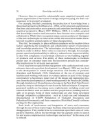
A selection of initial results are shown in Figures 10.2–10.5. Details of the
parameterization are available from the author. The horizontal axes can be
thought of asyears,the verticalaxesare in realprices.The figuresplotinvest-
ment, supply and demand over time. Figure 10.2 demonstrates that the
model is capable of generating investment bubbles and an initial boom – or
rapid expansion of capacity. It also shows a fluctuating expansion of activ-
ity in the long term. In this parameterization, long-term growth is deter-
mined bythe positivefeedbackof increases in supplyincreasing GDP,which
shifts the demand function upwards. The main features of the first four of
the stages of a Kondratiev wave are therefore shown. The slowing down due
to market saturation and increasing competitiveness in the long term will
require a more realistic modelling of demand allowing for market satur-
ation. This is discussed further in the conclusions.
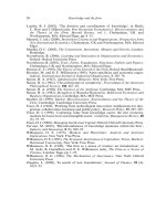
The model is capable of generating unstable behaviour and the chaotic
properties associated with nonlinear dynamic systems. Figures 10.3–10.5
demonstrate some of the range of behaviours that can be represented, even
by such a simple economic model. Figure 10.3 shows a cyclical growth path
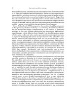
with an eventual collapse of the price. Figure 10.4 illustrates a case in which
the industry fails; the initial cost reduction is not great enough for demand
to take off. Finally, Figure 10.5 shows a case closely related to Figure 10.4.
After an initial decline, the cost and price reductions following a continued
relatively lowrateof investmentarejustsufficienttospark ademandgrowth.
262 Long-term technological change and the economy

Ϫ2000
0
2000
4000
6000
8000
Real prices
Time in
y
ears
10000
12000
14000
16000
Inv
Dem
Supp
114274053667992105 118 131 144
Figure 10.2 Investment, supply and demand over time
Simulating long-run technical change 263
Real prices
Time in years
Inv
Dem
Supp
Ϫ10000
Ϫ5000
0
5000
10000

15000
20000
25000
30000
35000
40000
1471013161922252831343740434649
Figure 10.3 Cyclical growth path with an eventual collapse of price
Figure 10.4 Industry failure
0
5
10
15
20
25
191725 33 41 49 57 65 73 81 89 97
Real prices
Time in years
Inv
Dem
Supp
6. CONCLUSIONS
This chapter has described a model of long term technological change,
based on the concept of Kondratiev waves. A descriptive explanation of
these waves from Freeman and Louçã (2001) has been summarized and
interpreted in a form that can be simulated with a dynamic numerical
model. The theory formalizes assumptions and processes required to gen-
erate Kondratiev waves, or long-term structural changes to the global
economy in a world of continuing technological revolutions. This has been
undertaken because the modelling of climate change and the associated

policy issues has to consider timescales of 50–100 years at least. Current
general macroeconomic models do not take into account these long-term
structural changes.
The dynamic simulation model that has been developed incorporates
some unusual features, which enable it to generate a wide variety of devel-
opment paths of an industry. It generates the boom phase of a Kondratiev
wave together with the investment bubbles that accompany the early
phases in a new wave. Its results are dependent on increasing returns to
scale in production costs, a lagged response to supply to the market situ-
ation and a rapid response of investment to profitability. The main short-
coming of this model is the linear demand response. Particularly in the
long term, markets become more competitive as they become saturated.
264 Long-term technological change and the economy
0
5
10
15
20
25
30
191725 33 41 49 57 65 73 81 89 97
Real prices
Time in years
Inv
Dem
Supp
Figure 10.5 Initial decline in cost and price following a relatively low rate
of investment are sufficient to spark demand growth
Therefore, a dynamic demand model allowing for a slowing down of the
increase in demand may deliver new insights into the growth behaviour.

Finally, the model must be calibrated against historical data on earlier
Kondratiev waves before it can be used as input into a long-term view of
economic change.
NOTE
1. This work is funded under the UK Tyndall Centre research theme ‘Integrating
Frameworks’.
REFERENCES
Alcamo, J., R. Leemans and E. Kreileman (eds) (1998), Global Change Scenarios of
the 21st Century: Results from the IMAGE 2.1 Model, London: Elsevier Science.
Arthur, W. B. (1994), Increasing Returns and Path Dependence in the Economy, Ann
Arbor, MI: University of Michigan Press.
Barker, T., J. Koehler and M. Villena (2002), ‘The costs of greenhouse gas abate-
ment: a meta-analysis of post-SRES mitigation scenarios’, Environmental
Economics and Policy Studies, 5 (2), 135–66.
Boyer, R. (1998), ‘Technical change and the theory of Regulation’, in G. Dosi,
C. Freeman, R. Nelson, G. Silverberg and L. Soete (eds), Technical Change and
Economic Theory, London: Pinter, pp. 67–94.
Cox, L.A. and D.A.Popken (2002), ‘A hybrid system-identification method for fore-
casting telecommunications product demands’, International Journal of
Forecasting, 18 (4), 647–71.
Criqui, P., N. Kouvaritakis, A. Soria and F. Isoard (1999), ‘Technical change and
CO
2
emission reduction strategies: from exogenous to endogenous technology in
the POLES model’, in P. Criqui (ed), Le progrès technique face aux défis énergé-
tiques du futur,Paris: Colloque européen de l’énergie de l’AEE, pp. 473–88.
David, P. A. (1993), ‘Path-dependence and predictability in dynamic systems with
local network externalities: a paradigm for historical economics’, in D. Foray and
C. Freeman (eds), Technology and the Wealth of Nations: The Dynamics of
Constructed Advantage, London: Pinter, pp. 208–31.

Day, R. H. (1994), Complex Economic Dynamics, Cambridge, MA and London:
MIT Press.
Dewick, P., K. Green and M. Miozzo (2004), ‘Technological change, industrial
structure and the environment’, Futures, 36 (3) (March), 267–93.
Dosi, G. (2000), Innovation, Organization and Economic Dynamics: Selected Essays,
Cheltenham, UK and Northampton, MA: Edward Elgar.
Freeman, C.and F.Louçã (2001),As TimeGoesBy,Oxford:OxfordUniversityPress.
Freeman, C. and L. Soete (1997), The Economics of Industrial Innovation,3rd edn,
London: Pinter.
Grübler, A., N. Nakicenovic and D. G. Victor (1999), ‘Dynamics of energy tech-
nologies and global change’, Energy Policy, 27 (5), 247–80.
Simulating long-run technical change 265
Nelson, R. R. and S. G. Winter (1982), An Evolutionary Theory of Economic
Change, Cambridge, MA: Harvard University Press.
Nordhaus, W. (1994), Managing the Global Commons: The Economics of Climate
Change, Cambridge, MA: MIT Press.
Perez, C. (1983), ‘Structural change and the assimilation of new technologies in the
economic and social system’, Futures, 15 (5), 357–75.
Silverberg, G. and L. Soete (eds) (1994), The Economics of Growth and Technical
Change: Technologies, Nations, Agents, Aldershot, UK and Brookfield, USA:
Edward Elgar.
266 Long-term technological change and the economy
11. Nonlinear dynamism of innovation
and knowledge transfer
Masaaki Hirooka
1
1. INTRODUCTION
This chapter proposes a new concept for innovation and knowledge trans-
fer. This approach offers a powerful tool to analyse ongoing innovation and
knowledge transfer in a rapidly changing global economy.

In the economic study of innovation so far, the diffusion of innovation,
market trends and the behaviour of firms have been intensively discussed.
There is, however, a long latent period of technology development before
the beginning of the diffusion of innovation. This technology development
period has not been sufficiently treated: it is a black box. This chapter
throws light on this technology development period and thus it becomes
possible to discuss an innovation paradigm as a comprehensive system con-
sisting of two periods of technology development and product diffusion.
One of the important findings of this study is the nonlinear nature of
innovation and knowledge transfer. The market for innovation products
reaches an ultimate maturity which never exceeds some limit. This rela-
tionship is well described by a logistic equation and we designate this locus
described by a logistic equation as a ‘trajectory’. A new finding presented
in this chapter is that technology development itself has a nonlinear nature
and can be described by a logistic equation. This is the main subject of this
chapter; and central to this is the knowledge transfer phenomenon in the
course of innovation.
This chapter is organized as follows. As a background, section 1 intro-
duces the concept of innovation diffusion as a logistics curve and offers evi-
dence of the diffusion coefficient of 17 products. Section 2 examines if the
logistic relationship holds for the technology (development) trajectory
and the (product) development trajectory: these two stages precede the
diffusion trajectory. Section 3 describes the three trajectories (collectively
referred to as an innovation paradigm) for electronics, biotechnology and
synthetic dyestuffs. Section 4 discusses the development trajectory in more
detail, focusing on the role of universities, venture business and national
267
systems of innovation with respect to electronics, biotechnology and
synthetic dyestuffs industries. Section 5 explains the implications of the
nonlinearity findings for innovation studies and section 6 presents some

concluding remarks.
2. LOGISTIC DYNAMISM OF INNOVATION
DIFFUSION
The economics of technological change has been discussed for a long time
since Schumpeter pointed out the importance of technological innovation
for economic development. Schumpeter (1939) ascribed the formation of
Kondratiev’s long waves to technological innovation in his book “Business
Cycles”. Since the Industrial Revolution, the economy has actually devel-
oped by various innovations which build economic infrastructures. The
diffusion of innovation to make a market is described by a logistic equation
as first pointed out by Griliches (1957) and many economists have con-
firmed this relationship, (for example Fisher and Pry, 1971; Mansfield,
1961, 1963, 1968; Marchetti, 1979, 1980, 1988; Marchetti et al., 1995, 1996;
Marchetti, 2002; Metcalfe, 1970; Modis, 1992; Nakicenovic and Grübler,
1991). Some authors, such as David (1975), Davies (1979), Metcalfe (1981,
1994), and Stoneman (1983) proposed modified models, to, for example,
explain the correlation between demand and supply in the economy.
Hirooka and Hagiwara(1992)extensively studied the diffusion of various
innovation products by expressing the diffusion phenomenon as a logistic
equation. This chapter begins by briefly discussing the results of these analy-
ses for the diffusion of innovation.
2.1 Logistic Equation
The logistic equation for product diffusion is expressed by the formula (1):
dy/dt ϭ a y (y
0
Ϫ y) (1)
where y is product demand at time t,
y
0
is the ultimate market size,

and a is a constant
The solution of this nonlinear differential equation is (2):
y ϭ y
0
/ [1 ϩ C exp (Ϫay
0
t)] (2)
268 Long-term technological change and the economy
If the logistic equation is expressed by the fraction F ϭ y/y
0
, the equa-
tions (1), (2) are represented by the formulae (3), (4):
dF/dt ϭ␣F (1ϪF ) (3)
F ϭ 1 / [ 1ϩC exp (Ϫ␣t)] (4)
This equation was transformed by Fischer and Pry (1971) to make a
linear relation on time t which is formulated by equation (5):
ln F / (1ϪF ) ϭ␣t Ϫ b (5)
The ultimate market size y
0
is determined by the flex point of the logis-
tic curve, y
0
/2,which is the secondary differential coefficient of (1), and
the adaptability of the logistic equation is examined by the linearity of the
Fisher–Pry plot. The ␣ is the diffusion coefficient of the product to the
market. If the time span between Fϭ0.1 and Fϭ0.9, is conveniently taken
to express the spread of the logistic curve, this is a conventional expression
of the time dependence of the product diffusion to the market as shown in
Figure11.1. This kind of treatment wasalso used by Marchetti(1979, 1988).
2.2 Logistic Dynamism of Product Diffusion

Before discussing the period of technology development, it is important to
describe a new concept of the diffusion process of innovation. Hirooka and
Nonlinear dynamism of innovation and knowledge transfer 269
⌬␶
0
0.1
0.5F
0.9
1.0 y
0
y
0
Figure 11.1 Logistic description of innovation and time span ⌬␶
Hagiwara (1992) have already examined the diffusion process by the above
procedure for 17 products including five bulk chemicals, four engineering
plastics, six electric appliances, crude steel, and automobiles. From the
determination of the flex point, a linear correlation of the Fisher–Pry plot
is examined as cited in Figures 11.2–11.5. The diffusion coefficient, ␣ was
determined and the results are shown in Table 11.1. The data are for the
Japanese market except that of ethylene for the USA on the basis of MITI
(2000) and UN (1996).
270 Long-term technological change and the economy
10
1
0.1
1960 70
Polypropylene
F
____
1ϪF

80 90
10
1
0.1
1960 70
Nylon resin
(polyamide)
80 90
Figure 11.3 Diffusion trajectories of plastics
10
1
0.1
0.02
1960 70
Ethylene (Japan)
F
____
1ϪF
80 90
10
1
0.01
1960 70
Ethylene (USA)
80 90
Figure 11.2 Diffusion trajectories of ethylene (petrochemicals)
These results clearly indicate that:
1. The diffusion of new products obeys a simple logistic equation during
sound economic conditions;
2. The diffusion is easily disturbed by economic turbulence, such as reces-

sions and wars, and sometimes the demand of products during turbu-
lence is sufficiently reduced as to dissociate it from the locus of the
logistic equation;
3. It is noteworthy that after the recession the diffusion of the product
resumes and takes up the same slope of the logistic curve as before the
recession. This strongly supports the fact that the diffusion of a product
has its own inherent trajectory with a definite diffusion coefficient.
Nonlinear dynamism of innovation and knowledge transfer 271
10
1
0.1
0.01
1960 70
Automobile
(4 wheeled, domestic)
80 9
0
10
1
0.1
1960 70
Crude steel
F
____
1ϪF
80 90
Figure 11.4 Diffusion trajectories of crude steel and automobile
F
____
1ϪF

0.01
0.1
1
10
Refrigerator
Colour TV
1960 1970 1980 1990
Microwave
oven
VCR
Facsimile
Word processor
Figure 11.5 Diffusion trajectories of electrical appliances
These results clearly indicate that the diffusion process of innovation
products is a kind of physical phenomenon with a definite diffusion
coefficient in thefield of innovation beyond the occurrence of economic tur-
bulences. The determination of diffusion coefficients is a first in the study of
innovation economics and gives an important basis for the consideration of
the logistic process of innovation which is carried out later. This issue is
deeply related to the nature of innovation per se.
2.3 How to Describe the Technology Development Period?
The diffusion of innovation productsrequires a longtime after the emergence
of radical technology. That is, innovation products appear in the market and
begin to diffuse after a long period of the development of the technology.
It is rather difficult to express concretely the states of technological devel-
opment. By analysingthe course of technologicaldevelopment,however,we
can draw some implications: in the early stages of technology, it is hard to
make rapid progress; afterreaching acertain level of technology, itdevelops
sharply; and at the final stage, the development of technology again slows
down. This progress suggests a kind of sigmoid curve.

2.4 Bibliometric Analysis of Technology Development Period
The output of technological development is patents and new products.
It is possible to describe the transition of the annual number of patent
applications and annual developments of new products in the course of
technology development. There are various case studies of the transition
272 Long-term technological change and the economy
Table 11.1 Diffusion coefficients of innovation products*
Product Diffusion Product Diffusion
coefficient ␣ coefficient ␣
Chemicals Crude steel 0.28
Ethylene 0.39 Automobile 0.32
Polypropylene 0.49 Electrical appliances
Polyvinyl chloride 0.23 Refrigerator 0.65
Polystylene 0.37 Colour TV 0.82
Nyron resin 0.24 Microwave oven 0.67
Polyacetal 0.27 VCR 0.73
Polycarbonate 0.24 Word processor 0.94
PPE 0.35 Facsimile 0.51
* Japanese market.
of patents and product development. Kaku (1986) intensively analysed
the number of new products commercialized in the dyestuff industry in
Germany and found a sharp distribution of the transition across the period
1850 to 1900. Achilladelis et al. (1990) described the transition of number of
patents in plastics and pesticide industries after World War II and indicated
sharp distribution of the trends in both cases. This chapter analyses these
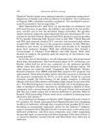
data by applying the Fisher–Pry plotand illustrates the results in Figure 11.6.
Figure 11.6 indicates sharp transitions and their Fisher–Pry plots clearly
give straight lines which are direct evidence that they obey a logistic
equation. Thus, a technology development period is illustrated as a logistic
S-curve having a definite time span. Recently, Andersen (2001) analysed the

transition for the number of US patents by classification for 100 years, from
1890 to 1990, and found that eight fields of chemicals,nine fields of electric-
als and electronics, 21 fields of mechanical engineering, two fields of trans-
portation, and four fields of nonindustrials exhibited trends expressed by a
logistic equation on the basis of regression analysis. She concluded that the
innovation process was expressed by a logistic equation as judged by a bib-
liometric analysis of patents.
From the point of view of knowledge development, Marchetti (1979,
1980) and Modis (1992) indicate that various human activities, for example
Nonlinear dynamism of innovation and knowledge transfer 273
10
1
0.1
F/1ϪF
1870 80
Fisher–Pry plot
90 1900
10
1
0.1
F/1ϪF
4
6
ϫ10
2
2
0
40
60
20

0
Cumulative number
1850 70
Number of new products
by German dye producers
90 1910
1950 60 70 80
10
1
0.1
F/1ϪF
1950 60 70 80
2
3
ϫ10
4
1
0
10
15
ϫ10
2
5
0
Annual new products
Cumulative number
1930 50
Pesticide patents
70 90
2

3
4
ϫ10
4
1
0
10
15
ϫ10
2
5
0
Annual applications
Cumulative number
Annual applications
1930 50
Pesticide patents
70 90
Source: Data from Achilladelis et al. (1990) and Kaku (1986).
Figure 11.6 Logistic nature of technology development
the music masterpieces of composers and the scientific papers of great schol-
ars, can be expressed by a sigmoid curve. Marchetti (1980) also disclosed that
the transition of various technological developments was expressed by a
logistic equation; that is, the efficiencies of steam engines, generation of elec-
tric power, electric lamps, and the ammonia production process. He also
pointed out that the number of chemical elements discovered was described
by a logistic equation in the course of the discovery. These findings strongly
support the logistic nature of technological development.
2.5 Evidence of the Logistic Nature of Technology Development
All of the above innovation processes are described by concrete quantities

such as numbers of patents, numbers of new products, and some physical
quantities. A problem is whether the real entity of technological develop-
ment itself, neither the number of patents nor physical properties of tech-
nology, can be expressed by a logistic equation or not. Technological
development is a phenomenon of knowledge transfer from person to
person in the field of human society. This is a kind of discrete behaviour.
The knowledge of technology, however, spreads over the relevant techno-
logical community and develops as if the knowledge continuously covers
the entire field. Results of technological developments described above are
only fruits materialized by such activity. The sigmoid curves of the innov-
ation process expressed by concrete quantities are likely to indicate that the
technological development itself has a logistic nature in the background. In
this subsection the author examines and confirms this issue for the two
cases of dyestuff development and pesticide development.
Kaku (1986) collected information regarding the historical development
of synthetic dye and data related to the number of new products. As
described in Figure 11.6, the number of annually developed new products
increased sharply from 1856 to the 1880s and decreased drastically towards
1900, obeying a logistic equation. Here, we checked the actual transition of
technology development and found that a series of new products are homo-
geneously scattered within the area of the developed number of new prod-
ucts as shown in Table 11.2 in which actual names of dyestuffs developed
are cited together with the number of new products by year. This compar-
ison in Table 11.2 clearly indicates that actual transition of new product
development fully meets the logistic locus of the number of new products.
More evidence of the logistic nature of product development is that the
actual distribution of individual pesticide products is scattered around
the logistic S-curve of the number of patents of pesticides as shown in
Figure 11.7.
These data reflect the fact that the technological development itself is dis-

274 Long-term technological change and the economy
tributed in the same locus as those described by concrete quantities of innov-
ation and can be concluded to have a logistic nature. That is, the bunch of the
discrete facts of developed technologies directly corresponds to the real locus
of technological development. Thus, the logistic curve of a technological
development can be determined by the concrete bunch of developed tech-
nologies and the size and positioning of the curve is determined by the time
span of the bunch. Of course, the vertical axis corresponds strictly to the level
of the technology or adegree of maturity.The nonlinear nature of innovation
indicates that there is no technology progress before or after the development
time span because of the breakthrough of the origin and the matur-
ation of technology after the time span.It is a very interesting and important
implication that all inventions of key technologies are gathered within a defi-
nite time span to make a bunch. A technology trajectory can be easily
identified by checking how inventionsaregatheredduring a definite timespan
and the time span of the trajectory can be determinedby knowingthefirstand
last core inventions in a bunch without measuring any quantitative mass.
Nonlinear dynamism of innovation and knowledge transfer 275
Table 11.2 Product development and number of new products in the
dyestuff industry in Germany
Year Developed dyestuff Number of new products
1856 Mauve 1
1859 Fuchsine 1
1863 Bismarck brown 1
1868 Alizalin 1
1871 5
1973 Eosine 2
1875 12
1877 Methylene blue 10
1878 20

1879 18
1880 Indigo 5
1883 23
1884 Congo red 10
1886 33
1895 22
1897 Indigo by naphthalene process 8
1899 8
1900 3
1901 Indanthrene 2
Source: Data from Kaku (1986).
2.6 How to Determine the Trajectory
It is important to know how to determine the trajectory. The actual method
of determining the trajectory should be defined. As described above, if the
measurement of the trajectory is carried out in the form of a Fisher–Pry
plot, the slope of the straight line corresponds to the time span in the
expression of the normalized scale of the vertical axis. As the logistic curve
spreads from minus infinity to plus infinity, we have to decide what the time
span is. We define the time span as the interval from Fϭ0.1 to Fϭ0.9.
Technologies and new products emerge discretely and not continuously.
This discrete phenomenon makes it possible to determine the time span.
Thus, if we look directly at the bunch of technologies arranged in order of
invention along the trajectory, we can define the first technology as Fϭ0.1
and the last one as Fϭ0.9. This kind of expression of time span has been
adopted already by Marchetti (1979, 1980, 1988; Marchetti et al., 1996). It
seems to be rather approximate but the actual determination was not so
complicated to do and was successfully achieved for more than 40 innov-
ations as shown in the next section. These results certainly reflect the non-
linear nature of the trajectory.
Thus, an actual determination method is illustrated in the case of the

innovation paradigm for electronics as shown in Table 11.3 and Figure 11.8.
According to the chronicle of electronics technologies from the 18th
276 Long-term technological change and the economy
1920
0
F
1
30
Cumulative number of patents
40 50 60 70 80 90 2000
Herbicide
Germicide
Insecticide
Source: Data from Sumitomo Chemical Co. (2002).
Note: The actual names of new pesticide products per annum were provided by courtesy
of the Pesticide Division, Sumitomo Chemical Company Ltd., Japan and marked on the S-
curve of annual developed numbers of pesticides.
Figure 11.7 Development of pesticides on patent distribution curve
century to the present (Kisaka, 2001), it can be easily summarized that the
origin of the technology trajectory was the discovery of the transistor by
Shockley et al. in 1948 and the last core technology was the completion of
Nonlinear dynamism of innovation and knowledge transfer 277
Table 11.3 Elements of technology trajectory of electronics
Year Inventor Invention Trajectory
1948 W. H. Brattain, Function of point Fϭ0.1
J. Bardeen contact transistor
1948 W. B. Shockley Patent of p-n junction
transistor
1949 W. B. Shockley, Establishment of
G. L. Pearson, p-n junction concept

M. Sparks
1949 W. B. Shockley Theory of p-n junction
transistor
1951 W. B. Shockley, Completion of
M. Sparks, p-n junction transistor
G. K. Teal
1952 W. B. Shockley Concept of unipolar
transistor
1953 G. C. Dacey, Unipolar field Trajectory
I. M. Ross effect transistor 1948–1973
1954 H. Krömer Drift type transistor ⌬␶ϭ25
1956 Charles A. Lee Diffused base transistor
1959 Jack S. Kilby Invention of solid
state circuit
1959 Jean A. Hoerni Silicon planar transistor
1960 Dawori Kaling, MOS transistor
M. M. Atalla
1961 R. W. Noyce Silicon planar
monolithic integrated circuit
1963 F. M. Wanlass, complementary metal oxide
C. T. Sah semi-conductor transistor
1965 Texas Instruments Schottky-cramped
transistor
1967 John T. Wallmark metal-nitride-oxide-semi-
conductor, Si-nitride-oxide
semiconductor
1971 Daglass L. Benzer ISO planar technology
1972 T. H. Philip Chang Electron beam stepper
1973 IBM Submicron lithography Fϭ0.9
Source: Data from Kisaka (2001) and some others.

submicron-lithography by IBM in 1973. Table 11.3 shows a series of core
technologies that were developed almost every year. The time span is simul-
taneously recognized as 25 years and the S-curve is instantly described as
shown in Figure 11.8. Each technology is placed on the curve by name and
year.
2.7 Determination of Time Span for Innovation Technologies
In order to confirm the finiteness of technological development, the author
has determined the time span of technological developments for more than
40 innovations since the Industrial Revolution to the present day as shown
in Figure 11.9. These bunches of technologies are identified by various data
from McNeil (1990), Yuasa (1989), other chronological technology hand-
books and textbooks. The identification of trajectory elements often
requires expert knowledge and the results were often confirmed by experts
from the relevant disciplines. The author has collected these data for more
than ten years. It was, however, surprising to find that after the elements
were confirmed, determining the time span was not so difficult, as the devel-
opment of innovative technologies clearly lined up within a definite time
span. This seems to be the first time an abstract phenomenon as technol-
ogy development is described by a concrete equation. This success is cer-
tainly ascribed to the nonlinear nature of innovation and the determination
only requires the time span of the spread of technologies to be measured
without cognition of the vertical axis, which is normalized as a fraction of
scale towards saturation at infinity.
278 Long-term technological change and the economy
48
Point contact transistor
p–n Junction transistor
Concept of unipolar transistor
Unipolar field effect transistor
Invention of solid state circuit

ISO planner technology
Electron beam stepper
Submicron lithography
MOS LSI
MNOS, Si nitride oxide memory
Schottky-cramped transistor
MOS IC
CMOS, Compensation type MOS transistor
Silicon plannar monolithic IC
MOS transistor
Silicon planar transistor
Diffused base transistor
Drift type transistor
49
51
52
53
54
56
59
60
61
63
64
65
67
68
71
72
73

1940
0
0.2
0.4
F
0.6
0.8
1.0
50 60 70 80 90
Figure 11.8 Identification of technology trajectory of electronics
Figure11.9 showsthat the time span of developed technologies wasaround
60 years at the age of the Industrial Revolution and is now shortened to 25 to
30 years. Kondratiev (1926) proposed a concept of a long wave of business
cycles and Schumpeter (1939) ascribed the business cycles to the cluster of
innovations. Hirooka (2002) provided direct evidence for Shumpeter’s postu-
lation and found that most innovations which had a major impact on the eco-
nomicinfrastructureswereintensively gatheredonthe upswingof Kondratiev
waves. Relatedto this finding, Figure 11.9 clearly showsclusters of innovation
trajectories which seem to be the origin of business cycles. That is, corre-
sponding to the IndustrialRevolution,thereis a cluster of spinning machines,
Nonlinear dynamism of innovation and knowledge transfer 279
1750 1800
IIIIII IV V
Innovation
clusters
Energy
Motive force &
transportation
Information &
communications

Inorganic
materials
Textiles
Polymers
Eng. plastics
Polymer synth.
Synthetic dyes
Petrochem.
Biotechnology
Genome eng.
Tissue eng.
Biotechnology
& organics
1850
50
Electric power
Internal
combustion
Aircraft
TV
Vacuum tube
Computers
Opto-
electronics
M
olecular
devices
Steam engine
Telegraph
Acid–alkali

Electrochem.
Steel
Superconductors
Super fibres
Precision
polymn.
Synth. fibres
Chem. fibres
Spinning
machine
Ceramic
sup.cond.
Fine ceramics
Iron
Telelphone
Oil cracking
Fuel cell
Nuclear energy
Solar cell
1900 1950 2000
IC
50 35 35 25 25
30
25
4060
60 60 50 50 30 30
25252535404050
60 40 40
35204040
35

2535
Figure 11.9 Determination of time span of technology development period
steam engines, blast furnaces for iron making, and acid/alkaline chemicals in
thelast half of 18thcentury.This clusterformsthefirstandsecond Kondratiev
waves. There is the second cluster located in the last half of the 19th century,
whichincludes steelmaking, the telephone,internalcombustion engines,elec-
tric power, and dyestuffswhich are the origin for the third Kondratiev wave.
The third cluster is that of innovation technologies for the economic growth
after the World War II: petrochemicals, oil cracking, aircraft, vacuum tubes,
computers, electrical appliances, synthetic plastics, synthetic fibres, and
rubbers. The fourth cluster is composed of high technologies for the contem-
porary industries: electronics, biotechnologies, fine ceramics, advanced com-
posites, and soon. Now, we are expecting thefifth wave andthese could bethe
cluster of multimedia, genome technologies, cell regeneration technologies,
nanomaterials, nanodevices, quantum computers, and so on. This is the first
finding that the origin of Kondratiev waves lies in the occurrence of clusters
of innovation technologies.
2.8 Technology Trajectory and Development Trajectory
Detailed analysis of innovation discloses that there are two kinds of trajecto-
ries during the technology development period. That is, since the first radical
invention or discovery, there is a series of core technologies that emerges in
line. This bunch is designated as the technology trajectory. After that, a series
of developments of new products follows. This is the development trajectory.
The first trajectory is that for the development of core technologies and the fol-
lowing trajectory is the development of new products;application technologies
and market development are also on the same trajectory. The two trajectories
formulated during the period of technology development period are easily
distinguished from each other because of the different nature of technologies.
The trajectory shown in Table 11.3 is a technology trajectory because of the
core technologies, while the development of new dyestuff products as given in

Table 11.2 and pesticides as shown in Figure 11.7 are development trajecto-
ries because they describe the development of new products. Most of the tra-
jectories depicted in Figure 11.9 are technology trajectories.
3. IDENTIFICATION OF AN INNOVATION
PARADIGM
3.1 Correlation of Technology Trajectory and Diffusion Trajectory
An innovation paradigm is composed of three trajectories: technology,
development, and diffusion trajectories, in this order. Interestingly, the
280 Long-term technological change and the economy
diffusion trajectory is seen to begin just after the technology trajectory is
almost complete, like a kind of cascade junction. This relation is an empir-
ical result, but it is important to describe the innovation paradigm and to
gain foresight in technology. Figures 11.10 and 11.11 depict typical exam-
ples of the interrelation between the actual technology trajectory and the
diffusion trajectory in various innovations such as energy development,
motive powers, and information and communication technologies. All of
these paradigms clearly indicate that the technology trajectory joins with
the diffusion trajectory in a cascade fashion. The source of data is the same
as in Figure 11.9 and industrial statistics.
3.2 Structure of an Innovation Paradigm
Now, let us describe the structure of the innovation paradigm consisting
of technology, development, and diffusion trajectories. The following
paragraphs describe the electronics, biotechnology, and synthetic dyestuff
paradigm.
The technology trajectory of the electronics innovation paradigm has
been introduced in Table 11.3 and Figure 11.8. The original invention
is the discovery of the transistor by Shockley et al. in 1948 and then core
inventions of integrated circuits by Kilby and Noyce,MOS IC, and steppers
followed. In 1973 IBM finally completed the technology of submicron-
lithography.This indicates thatthe timespan of the technology trajectory of

Nonlinear dynamism of innovation and knowledge transfer 281
Steam engine
1700 1750 1800
Steam engine
Railway network
1850
1900
Electric power
1800 1850 1900
Electric technology
Power supply
1950
2000
Internal engine & car
1800 1850 1900
Internal engine
Car production
1950 2000
Figure 11.10 Cascade of technology and diffusion trajectories
(1) Energy and motive powers
25 years from 1948 to 1973and we can illustrate thetechnology trajectory in
such a way. The development trajectory is the history of development of
integrated circuits which started from the completion of submicron-lithog-
raphyin1973.Thegrowthof DRAM formulatesthedevelopmenttrajectory
in which the degree of integration is advanced four times every three to four
years, known as Moore’s law. Theprogress isshown as16K DRAM in 1975,
64K in 1978, 1M in 1984 and 256M in 1992. This history of development of
new products forms a development trajectory with a time span of 25 years.
The development trajectory is also formulated by the history of develop-
ment of new devices like microprocessors and workstations, and also by the

history of the development of software. These histories of new develop-
ments constitute the development trajectory. The diffusion trajectory is
described by the actual consumption of semiconductor devices in the
market. The actual structure of the electronics paradigm is shown in Figure
11.12 in which the transition of the market size is represented by black dots.
The result of the study on the electronics paradigm indicates three trajecto-
ries each having the time span of 25 years.
The science of new biotechnologywas triggeredby Avery in 1944 with the
discoveryof deoxyribonucleic acid (DNA)astheoriginof genes.This is also
the origin of the technology trajectory of biotechnology and various dis-
coveries such as the helical structure of DNA, central dogma, decoding of
genes, and recombinant DNA, and the synthesis of insulin by E. coli (colon
282 Long-term technological change and the economy
1800 1850 1900 1950
2000
T
elegraph
techn.
Telegraph
Electric wave techn.
Electric wave techn.
Vacuum tube
Computer techn.
Personal com
pute
r
Electronics
Sem
iconductor
chip

Radio
Optoelectronics
Multimedia
networ
k
Communication
1800 1850 1900 1950
2000
Electronics
1800 1850 1900 1950
2000
Computer
Figure 11.11 Cascade of technology and diffusion trajectories
(2) Information and communications technologies
bacillus), which together constitutethe technology trajectory that lasted for
35 years. The development trajectory started with the development for the
commercialization of human insulin by E. coli and the various biotechnol-
ogyproducts that developed along the trajectory. The biotechnology para-
digm is shown in Figure 11.13.
The first synthetic dyestuff wasinvented by Perkin in 1856 at the London
College of Chemistry and until the early 20th century many more synthetic
dyestuffswere developed on as shown in Figure 11.6 and Table 11.2. Such
progress is described as the development trajectory. The technology
trajectory corresponds to the development trajectory and is the history of
organic chemistry, mostly at universities, starting from the identification of
organic substances by Wöhler to the establishment of organic chemistry by
Kekulé. The actual sales of dyestuffs describe the diffusion trajectory. The
innovationparadigmof syntheticdyestuffsisgivenbyFigure11.14.The time
span of each of these trajectories is 40 years.
4. IMPLICATIONS OF THE LOGISTIC DYNAMISM

OF INNOVATION
The innovation paradigm consists of three trajectories and has a logistic
nature which indicates that every trajectory reaches an ultimate level of
saturation within a definite time period. Each trajectory plays its own role
Nonlinear dynamism of innovation and knowledge transfer 283
Submicron lithography
1G
4G
Windows95
Windows (Microsoft)
UNIX International
Lotus-1, 2, 3
Diffusion trajectory
UNIX (AT&T)
4K
16K
Intel 8008
64K DRAM
256K
Workstation (SUN-1)
Macintosh (Apple)
1M
4M
Developm
ent trajectory
Technology trajectory
Microprocessor SPARC (SUN)
RISC microprocessor
Personal computor
Basic (Microsoft)

ALTO (XEROX)
BDS (UNIX)
MS-DOS (Microsoft)
64M
256M
16M
73
72
71
68
95
90
89
88
87
86
84
82
82
82
80
79
78
75
74
75
73
69
67
65

64
63
61
60
59
59
56
54
53
52
51
48
49
Electron beam stepper
Schottky-cramped transistor
MOS • IC
Invention of solid state circuit
Junction FET
Idea of unipolar transistor
P–N junction transistor
P–N junction theory
Point contact transistor
P–N junction
1930
0
F
1
40 50 60 70 80 90 2000 1
0
⌬␶ϭ 25

⌬␶ϭ 25
⌬␶ϭ 25
Drift type transistor
Diffused base transistor
Silicon planar transistor
MOS transistor patent
Silicon planar integrated circuit
CMOS (compensation type MOS)
MOS LSI
MNOS (Si-nitride oxide) memory
ISO planar technology patent
Source: Data from Kisaka (2001), MITI (2000), Shimura (1992), and others.
Figure 11.12 Innovation paradigm of electronics
and the actors involved are also different. In this sense, knowledge transfer
across the trajectories and within a trajectory as well is also very important.
The technology trajectory establishes core technologies,the development tra-
jectory develops new products and the diffusion trajectory focuses on sales.
Each trajectory has its own role. Among these trajectories, the development
trajectory is the most important in the sense of innovation. In this section,
some characteristics and roles of the development trajectory are discussed.
4.1 Role of Universities in the Innovation Paradigm
The technology trajectory is often composed of the fruits of basic research
that ismostlycarried outatuniversities,whichmeansscientific research.The
technology trajectory of synthetic dyestuffsisthe outcome of pure research
in organic chemistry that was carried out at universities. Biotechnology was
based through basic research into gene science at universities, which started
with the discovery of genes by Avery and ended with the great achievement
of recombinant DNA by Cohen and Boyer. The technology trajectory of
polymer science is also a kind of scientific trajectory in which research was
mostly carried out at universities, starting with the concept of macromole-

cules by Staudinger. The technology trajectory of electronics is formulated
mostly by research at firms but rich in basic flavour. Further, many universi-
ties were involved, in particular Stanford University in establishing elec-
284 Long-term technological change and the economy
Source: Data from Lewin (1983), JBA (2003), Walker & Gingold (1985) and others.
Figure 11.13 Innovation paradigm of biotechnology
DNA as gene
501940
0
1
F
60 70 80 90 2000 10 20
Structure of insulin
Enzyme for DNA synthesis
Cell fusion
Decoding of genes as triplet coding
Cloning carrot cells by tissue culture
␥-Interferon
⌬␶ϭ 30⌬␶ϭ 30⌬␶ϭ 35
TPA
Sodium diuretic peptide
Insulin growth factor I
Hepatitis A vaccine
Blood coagulation factor VIII
Interleukin·2 derivatives
Human insulin by E. coli
Human interferon by E. coli
Production of human insulin
Human growth hormone
␣-Interferon

Hepatitis B vaccine
Erythropoietin
Granulocyte colony·stimulating factor
Human insulin by E. coli
Monoclonal antibody
Recombinant DNA technology
Central dogma
Double helix of DNA
44
51
82
86
87
88
89
91
92
95
85
80
78
53
56
57
58
61
69
73
75
78