introduction to spss RESEARCH METHODS & STATISTICS HANDBOOK PHẦN 2 pdf
Bạn đang xem bản rút gọn của tài liệu. Xem và tải ngay bản đầy đủ của tài liệu tại đây (154.87 KB, 10 trang )
11
SECTION II
PRACTICALS
12
WEEK 1: Thursday October 3
th
Introduction to SPSS
SPSS is the primary package for running any statistical procedures outside of the
MDS packages. In addition to providing outputs for various analyses, SPSS allows
the user to manipulate the data in a variety of ways and to produce various graphs and
figures that can be added into documents.
In this practical, you will be asked to open and search through a data matrix, and enter
and code data. The procedure for the exercises in this practical involves going
through the steps for each analysis using the data file family.sav.
Where is Family.sav?
The first thing you must do is copy family.sav from the N: drive on your computer to
the M: drive (which is your own personal account). To do this you must create a
folder on your M: drive into which the family.sav file will go. You should be
looking at a screen with a number of icons on it. In the top left-hand corner is an icon
called my computer. Double-click on this icon.
Find the M: drive and double-click on it. You should now see a window containing a
number of folders. Go to FILE, then NEW and choose FOLDER. A new folder
should appear in the bottom of the window labelled „New Folder‟. Call your new
folder „Survey‟ and ENTER. After you have done this, go to FILE and then
CLOSE.
Now, within the same window double-click on your N: drive. Within that drive you
will see a folder with title SPSSEGS (standing for SPSS example files). Double-click
on this folder. Within this folder there is a file labelled family.sav. This is the file
you want to copy into your „Survey‟ folder on your M: drive. So, single click on
family.sav and go to EDIT and then COPY.
Go back to your M: drive by shutting down the N: drive. (click on the X in the right
hand corner of your N: drive window). Double-click on your M: drive and double-
click on the folder Survey. Survey should be empty. Go to EDIT and then PASTE.
Now you should see the file family.sav.
Exploring the Data Editor Window
Start SPSS for windows by double-clicking on the SPSS icon. Once the program has
been opened a window will appear in the middle of the screen with a number of
options to choose from. You want to select OPEN AN EXISTING DATA
SOURCE.
Go to the directory Survey in your M: drive. Find the file family.sav and double-
click on it. The values from the family.sav file should now appear in the Data Editor
window. Click on the middle button in the top right hand corner of the window to
maximise the size of the window. Once the file is open you will see two sheets at the
bottom of the window. One is labelled DATA VIEW and the other is labelled
13
VARIABLE VIEW. You want to stay on the data view sheet. Click on the VALUE
LABELS (in bold rectangle below) button on your tool bar (it is 2
nd
from the right).
This will toggle between value labels (numeric and string (words)). Scroll through
the data to answer the following questions:
1. What is the name of the last variable in the data matrix?
2. What is the case number of the last case?
3. What is the value of IDNUM for the last case?
4. What is Robert‟s date of birth?
5. What is Jack‟s marital status?
If you click on a cell when value labels are displayed in the DATA VIEW
WINDOW a scroll bar will appear to provide an indication of the options (variable
labels) used in the coding framework. Using this feature, please answer the following
questions:
What are the labels for CAR?
What are they for MORTGATE?
What are they for NAME? Is there a problem with NAME? What is it?
14
The variable view sheet
In order to view how a variable has been defined in terms of its name, variable label,
value labels and user-missing values you have to click on the sheet VARIABLE
VIEW.
Please answer the following questions. Do not forget to use the scroll bars on the
bottom and on the right side of the variable view window to find your answers.
What is the variable label for DATEBLT?
What are the values and value labels for MARSTAT? (hint: click on the grey box)
What is the user-missing value for NCARS?
Click on this Sheet
15
Coding and Entering Data
Open up a new Data Editor window by going to FILE, then NEW and save DATA to
M: drive. Below is a questionnaire regarding leisure activity and a coding scheme.
Your task is to set up the Data Editor Window and then enter the data below.
Leisure Activity Questionnaire
1. What is your first name?
2. What is your sex? M = male, F = female
3. What is your marital status?
1 = married 4 = widowed
2 = cohabiting 5 = divorced
3 = single 6 = separated
4. Do you watch sports? 1 = yes 2 = no 3 = do not know
5. Do you play sports? 1 = yes 2 = no 3 = do not know
6. Do you visit the seaside? 1 = yes 2 = no 3 = do not know
7. Do you go to films? 1 = yes 2 = no 3 = do not know
8. Do you go pop concerts? 1 = yes 2 = no 3 = do not know
Coding Framework
Variable Name
Format
Variable Label
Coding Details/Labels
IDNUM
NUMERIC
IDENTIY NUMBER
Unique Number for Each Person
NAME
STRING
FIRST NAME
Enter First Characters of Name
SEX
STRING
SEX
M = male F = Female
AGE
NUMERIC
AGE IN YEARS
Enter age in years (-9 = Missing)
MARSTAT
NUMERIC
MARITAL STATUS
1=married 4=widowed
2=cohabiting 5=divorced
3 = single 6 = separated
WATCHSP
NUMERIC
WATCHES SPORTS
1 = yes 2 = no 3 = do not know
PLAYSP
NUMERIC
PLAYS SPORTS
1 = yes 2 = no 3 = do not know
VISITSEA
NUMERIC
VISITS SEASIDE
1 = yes 2 = no 3 = do not know
GOTOFILM
NUMERIC
GOES TO FILMS
1 = yes 2 = no 3 = do not know
GOTOPOP
NUMERIC
GOES TO POP CONCERTS
1 = yes 2 = no 3 = do not know
Data
IDNUM
NAME
SEX
AGE
MARSTAT
WATCHSP
PLAYSP
VISITSEA
GOTOFILM
GOTOPOP
101
MARGARET
F
87
4
201
JACK
M
62
1
1
2
1
2
2
202
JOSIE
F
1
2
2
1
2
2
301
NANCY
F
60
5
1
2
1
2
2
503
VICTORIA
F
11
-9
2
1
1
1
3
1002
JOHN
M
31
2
1
3
1
1
1
You should have a clean window in front of you (i.e., there should not be any data in
the spreadsheet). You now have to set up each column of your data matrix so that you
can eventually enter in your data. The first column will hold IDNUM. To enter
IDNUM into the data view sheet you need to go to the VARIABLE VIEW window.
16
In fact, defining and labelling all of your variables must be done in your variable view
sheet.
In the first Row (horizontal) you can label and define your first variable IDNUM.
Using the coding framework above enter in the appropriate information. Type in the
variable IDNUM under NAME. The TYPE of variable is NUMERIC (you are
entering a number) and under DECIMALS, using the scroll bar, choose 0 decimal
places. Under the heading LABELS you want to type in the definition of the
variable. Make sure this definition clearly defines the variable to avoid confusion.
Depending upon the type of data (i.e., nominal, ordinal, ratio, or interval) you are
measuring you may have to add VALUES. In the case of IDNUM (identify number)
there is only one unique number, therefore you do not have to define the variable. So,
under VALUES, you should have chosen none. However in defining nominal data
such as SEX (your third variable to enter) you would have to define male as „M‟ and
female as „F‟.
For IDNUM there are no missing values therefore you choose none. The heading
COLUMNS will give you the opportunity to define the width of your column.
Choose a width of 6. The ALIGN value allows you to determine the positioning of
your data in the cell. It may be right, left or centred. In the last column heading is
MEASURE. This column allows you to define the type of data you are working
with. With IDNUM you are working with scale data.
When you define variables such as NAME (i.e., the name of the subject), you want
the TYPE of variable to be STRING, the WIDTH should be 10 (refers to the number
of characters to appear in the name). Using the coding framework below define the
variable NAME.
When you define variables such as sex (nominal data) you want to add value labels in
the column called VALUES. If you click on the cell a value labels window will
appear. Across from value you should type your value M and across from the value
label type male and then click on add. Then you should enter F in the value box and
female in the value label box. Once you have made these changes you can move back
to the DATA VIEW window and view the changes.
Return to the VARIABLE VIEW window and define the numeric variable AGE in
the next row. It has no decimal places, and it requires a missing value of –9 to identify
cases where a response is not given. To assign a user-missing value of –9 click on the
MISSING column. A missing values window will appear. Click on Discrete missing
values and enter –9 in the first box. Set up a variable label and a value for –9 as
shown in the coding scheme for your questionnaire. Now, do the same for the
numeric value MARSTAT in the next row. This too is numeric with no decimal
places, has a user-missing value of –9 and requires a variable label and several value
labels as shown in the coding scheme.
The remaining 5 variables also need to be defined. To avoid defining each variable
separately you should define the first variable WATCHSP and then copy the cells to
the remaining four below. To do this go to the cell you want to repeat (i.e., the value
17
labels) and click on EDIT, COPY and then move to the cell where you want the same
definition and then go to EDIT and PASTE.
When you have finished entering all of the data save it into an SPSS file by selecting
FILE, SAVE and clicking on the folder Survey in your M: drive. Save the file under
any name you want (e.g., Person.sav). Exit from SPSS and log off.
18
WEEK 2: October 10
th
Descriptive Statistics, Charts & Manipulating Data in the
Matrix
This practical is divided into two sections. The first section is intended to familiarise
you on how to run commands to calculate descriptive statistics and to graph your data.
The second section aims to show you how to compute re-code, filter and delete your
data.
Section I: Descriptive Statistics & Charts
We shall estimate descriptive statistics for the three variables: TYPACCM,
DATEBLT, & NADULTS.
Question: Are these variables nominal (non-ordered categories), ordinal (with ordered
categories) or metrical (on a measure scale with well-defined differences between
values)? Hint: The second variable is not so obvious.
To run the descriptive statistics click on ANALYZE, DESCRIPTIVE STATISTICS
and then FREQUENCIES. In the left box there should be a list of all the variables
that are present in the spreadsheet. Highlight TYPACCM and click the arrow between
the boxes to move it into the box labelled „variables‟. Continue this for the other two
variables. A shorter route to move the variables to the „variables box‟ would be to
double-click on the variables when they are in the left box - removing the variables
may be accomplished in the same manner.
After the three variables are in the „variables box‟, click on STATISTICS at the
bottom of the box. Within the „Frequencies: Statistics‟ box there are several options.
Tick the boxes for MEAN, MEDIAN & MODE on the right hand side. In addition,
tick the boxes for STANDARD DEVIATION (Std. Deviations) & RANGE. After,
click on the continue button and wait for the data to process and for the output
window to appear.
Answer the follow questions:
What is the most useful measure of central tendency for each of the three variables?
What are the sample values?
What is the maximum value for NADULTS? Does this appear to be correct?
Now, try re-estimating the descriptive statistics for NADULTS, only this time without
the case with the unusual value. Select DATA and then SELECT CASES. Within
the Select Cases make sure under the „Unselected Cases‟ that the „Filtered‟ box is
ticked. Then select the IF CONDITION IS SATISFIED option and click on the IF
button. Move the variable NADULTS to the adjacent box by either double-clicking
on it or by clicking on the variable and moving it across using the arrow.
After the variable label use the calculator provided to type less than (<) the value of
19
the unusual variable. After this hit continue and then OK to return to the spreadsheet.
Answer the follow questions:
Has the case with the unusual value been barred off?
Which case is it?
Now, re-run the Frequencies command for NADULTS only and record the mean,
median & mode with and without the case included.
Which descriptive statistic is most affected by the unusual variable?
Graphing your Results
Histograms
Histograms are statistical diagrams that show the distribution of variables. In a
histogram, values are grouped together in intervals and a bar is drawn for each
interval whose area is proportional to the number of cases in the interval.
To generate a histogram select GRAPHS and HISTOGRAM
Then move the variable HEIGHT into the variable box. In the same box, click the
„display normal curve‟ box and then hit OK.
Upon examining the output window that contains the graph answer the following
question:
Do you think HEIGHT has a normal distribution, or would you run other tests?
Go back to the data editor window, select GRAPHS and HISTOGRAM and run the
same command as done using the HEIGHT variable but with WEIGHT.
From the histogram, would you say that the variable WEIGHT has a normal
distribution or would you try other tests?
Are there any differences between the two histograms?
Scatter plots
Scatter plots show the joint behaviour of two (or more) variables in a diagram.
Values of one of the variables are plotted against values of another, the two variables
usually being metrical. A scatter plot usually shows much more about the behaviour
of the variables than descriptive statistics like correlation.
Scatter plots are also drawn using the GRAPHS command. Click on GRAPHS then
SCATTERPLOT then on the SIMPLE option and then click on the DEFINE
button. Select WEIGHT for the Y-axis and HEIGHT for the X-axis. In a scatter plot,
20
if one of the variables is thought to depend on the other, it is plotted on the vertical Y-
axis. Here, we think that weight depends on height, therefore, weight is plotted on the
Y- axis.
In addition, select SEX for „select markers by‟. This will allow you to identify points
on the scatter plot by sex, as males and females tend to have different heights and
weights. Run the command and look at the scatter plot in the chart carousel window.
Can you see any difference between the males and the females in terms of heights and
weights?
To edit the chart simply double-click on it. Now we shall try fitting simple linear
regression lines to the data. Select CHART then OPTIONS and FIT LINES (Select
Subgroups) and FIT OPTIONS. Make sure linear regression has been highlighted
and then click-on „continue‟. There should be two different lines for males and
females.
What can you say about the slopes of the two regression lines?
Can you see any difference now between the males and the females in terms of
heights and weights?
The markers used to distinguish males and females are drawn in different colours, but
the difference is not very clear. It will become less clear if you print out the scatter
plot on a monochrome printer! Click on any marker in the plot: all markers of that sex
become highlighted in black squares. Then click on the icon depicting a
„crayon/pencil‟ to change the colour of the marker/symbol. To change the symbol
simply click on FORMAT and then MARKER. There you should have several
options of changing the type and size of the symbol. After making the chosen changes
hit „Apply‟ and „Close‟.
Editing a High Resolution Chart
Generate a high-resolution chart, a histogram, to try out some of the editing features.
Histograms are used for metric or quantitative variables, like AGE, which takes on
values along a scale. There are generally too many distinct values to make it worth
drawing a bar chart. Instead, the values are grouped into intervals or bands and a bar
is drawn for each interval. The area of each bar is proportional to the number of cases
with values in the interval.
Still using family.sav select GRAPHS and then HISTOGRAM. Select HWRATIO
for the variable box and click OK. A histogram for HWRATIO is added to the Chart
Carousel Window. The histogram shows some descriptive statistics for the variable
too.
What are the sample mean and standard deviation for HWRATIO?