Numerical Methods in Engineering with Python Phần 8 pot
Bạn đang xem bản rút gọn của tài liệu. Xem và tải ngay bản đầy đủ của tài liệu tại đây (495.72 KB, 44 trang )
P1: PHB
CUUS884-Kiusalaas CUUS884-08 978 0 521 19132 6 December 16, 2009 15:4
297 8.2 Shooting Method
EXAMPLE 8.4
x
w
0
v
L
The displacement v of the simply supported beam can be obtained by solving
the boundary value problem
d
4
v
dx
4
=
w
0
EI
x
L
v =
d
2
v
dx
2
= 0atx = 0 and x = L
where EI is the bending rigidity. Determine by numerical integration the slopes at
the two ends and the displacement at mid-span.
Solution Introducing the dimensionless variables
ξ =
x
L
y =
EI
w
0
L
4
v
transforms the problem to
d
4
y
dξ
4
= ξ y =
d
2
y
dξ
2
= 0atξ = 0 and 1
The equivalent first-order equations and the boundar y conditions are (the prime de-
notes d/dξ )
y
=
⎡
⎢
⎢
⎢
⎣
y
0
y
1
y
2
y
3
⎤
⎥
⎥
⎥
⎦
=
⎡
⎢
⎢
⎢
⎣
y
1
y
2
y
3
ξ
⎤
⎥
⎥
⎥
⎦
y
0
(0) = y
2
(0) = y
0
(1) = y
2
(1) = 0
The program listed next is similar to the one in Example 8.1. With appropri-
ate changes in functions
F(x,y), initCond(u), and r(u) the program can solve
boundary value problems of any order greater than 2. For the problem at hand we
chose the Bulirsch–Stoer algorithm to do the integration because it gives us control
over the printout (we need y precisely at mid-span). The nonadaptive Runge–Kutta
method could also be used here, but we would have to guess a suitable step size h.
As the differential equation is linear, the solution requires only one iteration with
the Newton–Raphson method. In this case, the initial values u
1
= dy/dξ |
x=0
and u
2
=
d
3
y/dξ
3
|
x=0
are irrelevant; convergence always occurs in one iteration.
#!/usr/bin/python
## example8_4
from numpy import zeros,array
from bulStoer import *
P1: PHB
CUUS884-Kiusalaas CUUS884-08 978 0 521 19132 6 December 16, 2009 15:4
298 Two-Point Boundary Value Problems
from newtonRaphson2 import *
from printSoln import *
def initCond(u): # Initial values of [y,y’,y",y"’];
# use ’u’ if unknown
return array([0.0, u[0], 0.0, u[1]])
def r(u): # Boundary condition residuals see Eq. (8.7)
r = zeros(len(u))
X,Y = bulStoer(F,xStart,initCond(u),xStop,H)
y = Y[len(Y) - 1]
r[0] = y[0]
r[1] = y[2]
return r
def F(x,y): # First-order differential equations
F = zeros(4)
F[0] = y[1]
F[1] = y[2]
F[2] = y[3]
F[3] = x
return F
xStart = 0.0 # Start of integration
xStop = 1.0 # End of integration
u = array([0.0, 1.0]) # Initial guess for {u}
H = 0.5 # Printout increment
freq = 1 # Printout frequency
u = newtonRaphson2(r,u,1.0e-4)
X,Y = bulStoer(F,xStart,initCond(u),xStop,H)
printSoln(X,Y,freq)
raw_input("\nPress return to exit")
Here is the output:
x y[0] y[1] y[2] y[3]
0.0000e+000 0.0000e+000 1.9444e-002 0.0000e+000 -1.6667e-001
5.0000e-001 6.5104e-003 1.2153e-003 -6.2500e-002 -4.1667e-002
1.0000e+000 -2.4670e-014 -2.2222e-002 -2.7190e-012 3.3333e-001
Noting that
dv
dx
=
dv
dξ
dξ
dx
=
w
0
L
4
EI
dy
dξ
1
L
=
w
0
L
3
EI
dy
dξ
P1: PHB
CUUS884-Kiusalaas CUUS884-08 978 0 521 19132 6 December 16, 2009 15:4
299 8.2 Shooting Method
we obtain
dv
dx
x=0
= 19.444 × 10
−3
w
0
L
3
EI
dv
dx
x=L
=−22.222 ×10
−3
w
0
L
3
EI
v|
x=0.5L
= 6.5104 × 10
−3
w
0
L
4
EI
which agree with the analytical solution (easily obtained by direct integration of the
differential equation).
EXAMPLE 8.5
Solve
y
(4)
+
4
x
y
3
= 0
with the boundary conditions
y(0) = y
(0) = 0 y
(1) = 0 y
(1) = 1
and plot y versus x.
Solution Our first task is to handle the indeterminacy of the differential equation at
the origin, where x = y = 0. The problem is resolved by applying L’H
ˆ
ospital’s rule:
4y
3
/x → 12y
2
y
as x → 0. Thus, the equivalent first-order equations and the bound-
ary conditions that we use in the solution are
y
=
⎡
⎢
⎢
⎢
⎣
y
0
y
1
y
2
y
3
⎤
⎥
⎥
⎥
⎦
=
⎡
⎢
⎢
⎢
⎢
⎢
⎢
⎣
y
1
y
2
y
3
−12y
2
0
y
1
if x = 0
−4y
3
0
/x otherwise
⎤
⎥
⎥
⎥
⎥
⎥
⎥
⎦
y
0
(0) = y
1
(0) = 0 y
2
(1) = 0 y
3
(1) = 1
Because the problem is nonlinear, we need reasonable estimates for y
(0) and
y
(0). Based on the boundary conditions y
(1) = 0 and y
(1) = 1, the plot of y
is
likely to look something like this:
1
1
1
y
"
x
0
P1: PHB
CUUS884-Kiusalaas CUUS884-08 978 0 521 19132 6 December 16, 2009 15:4
300 Two-Point Boundary Value Problems
If we are right, then y
(0) < 0 and y
(0) > 0. Based on this rather scanty infor-
mation, we try y
(0) =−1 and y
(0) = 1.
The following program uses the adaptive Runge–Kutta method (
run kut5)for
integration:
#!/usr/bin/python
## example8_5
from numpy import zeros,array
from run_kut5 import *
from newtonRaphson2 import *
from printSoln import *
def initCond(u): # Initial values of [y,y’,y",y"’];
# use ’u’ if unknown
return array([0.0, 0.0, u[0], u[1]])
def r(u): # Boundary condition residuals see Eq. (8.7)
r = zeros(len(u))
X,Y = integrate(F,x,initCond(u),xStop,h)
y = Y[len(Y) - 1]
r[0] = y[2]
r[1] = y[3] - 1.0
return r
def F(x,y): # First-order differential equations
F = zeros(4)
F[0] = y[1]
F[1] = y[2]
F[2] = y[3]
if x == 0.0: F[3] = -12.0*y[1]*y[0]**2
else: F[3] = -4.0*(y[0]**3)/x
return F
x = 0.0 # Start of integration
xStop = 1.0 # End of integration
u = array([-1.0, 1.0]) # Initial guess for u
h = 0.1 # Initial step size
freq = 1 # Printout frequency
u = newtonRaphson2(r,u,1.0e-5)
X,Y = integrate(F,x,initCond(u),xStop,h)
printSoln(X,Y,freq)
raw_input("\nPress return to exit")
P1: PHB
CUUS884-Kiusalaas CUUS884-08 978 0 521 19132 6 December 16, 2009 15:4
301 8.2 Shooting Method
The results are:
x y[0] y[1] y[2] y[3]
0.0000e+000 0.0000e+000 0.0000e+000 -9.7607e-001 9.7131e-001
1.0000e-001 -4.7184e-003 -9.2750e-002 -8.7893e-001 9.7131e-001
3.9576e-001 -6.6403e-002 -3.1022e-001 -5.9165e-001 9.7152e-001
7.0683e-001 -1.8666e-001 -4.4722e-001 -2.8896e-001 9.7627e-001
9.8885e-001 -3.2061e-001 -4.8968e-001 -1.1144e-002 9.9848e-001
1.0000e+000 -3.2607e-001 -4.8975e-001 -6.7428e-011 1.0000e+000
x
0.00 0.20 0.40 0.60 0.80 1.00
y
-0.350
-0.300
-0.250
-0.200
-0.150
-0.100
-0.050
0.000
By good fortune, our initial estimates y
(0) =−1 and y
(0) = 1 were very close to the
final values.
PROBLEM SET 8.1
1. Numerical integration of the initial value problem
y
+ y
− y = 0 y(0) = 0 y
(0) = 1
yielded y(1) = 0.741028. What is the value of y
(0) that would result in y(1) = 1,
assuming that y(0) is unchanged?
2. The solution of the differential equation
y
+ y
+ 2y
= 6
with the initial conditions y(0) = 2, y
(0) = 0, and y
(0) = 1yieldedy(1) =
3.03765. When the solution was repeated with y
(0) = 0 (the other conditions
being unchanged), the result was y(1) = 2.72318. Determine the value of y
(0) so
that y(1) = 0.
3. Roughly sketch the solution of the following boundary value problems. Use the
sketch to estimate y
(0) for each problem.
(a) y
=−e
−y
y(0) = 1 y(1) = 0.5
(b) y
= 4y
2
y(0) = 10 y
(1) = 0
(c) y
= cos(xy) y(0) = 0 y(1) = 2
P1: PHB
CUUS884-Kiusalaas CUUS884-08 978 0 521 19132 6 December 16, 2009 15:4
302 Two-Point Boundary Value Problems
4. Using a rough sketch of the solution estimate of y(0) for the following boundary
value problems.
(a) y
= y
2
+ xy y
(0) = 0 y(1) = 2
(b) y
=−
2
x
y
− y
2
y
(0) = 0 y(1) = 2
(c) y
=−x(y
)
2
y
(0) = 2 y(1) = 1
5. Obtain a rough estimate of y
(0) for the boundary value problem
y
+ 5y
y
2
= 0
y(0) = 0 y
(0) = 1 y(1) = 0
6. Obtain rough estimates of y
(0) and y
(0) for the boundary value problem
y
(4)
+ 2y
+ y
sin y = 0
y(0) = y
(0) = 0 y(1) = 5 y
(1) = 0
7. Obtain rough estimates of
˙
x(0) and
˙
y(0) for the boundary value problem
¨
x + 2x
2
− y = 0 x(0) = 1 x(1) = 0
¨
y + y
2
− 2x = 1 y(0) = 0 y(1) = 1
8.
Solve the boundary value problem
y
+
(
1 −0.2x
)
y
2
= 0 y(0) = 0 y(π/2) = 1
9.
Solve the boundary value problem
y
+ 2y
+ 3y
2
= 0 y(0) = 0 y(2) =−1
10.
Solve the boundary value problem
y
+ sin y + 1 = 0 y(0) = 0 y(π) = 0
11.
Solve the boundary value problem
y
+
1
x
y
+ y = 0 y(0) = 1 y
(2) = 0
and plot y versus x. Warning : y changes very rapidly near x = 0.
12.
Solve the boundary value problem
y
−
1 −e
−x
y = 0 y(0) = 1 y(∞) = 0
and plot y versus x. Hin t: Replace the infinity by a finite value β. Check your
choice of β by repeating the solution with 1.5β. If the results change, you must
increase β.
P1: PHB
CUUS884-Kiusalaas CUUS884-08 978 0 521 19132 6 December 16, 2009 15:4
303 8.2 Shooting Method
13. Solve the boundary value problem
y
=−
1
x
y
+
1
x
2
y
+ 0.1(y
)
3
y(1) = 0 y
(1) = 0 y(2) = 1
14.
Solve the boundary value problem
y
+ 4y
+ 6y
= 10
y(0) = y
(0) = 0 y(3) − y
(3) = 5
15.
Solve the boundary value problem
y
+ 2y
+ sin y = 0
y(−1) = 0 y
(−1) =−1 y
(1) = 1
16.
Solve the differential equation in Prob. 15 with the boundary conditions
y(−1) = 0 y(0) = 0 y(1) = 1
(this is a three-point boundary value problem).
17.
Solve the boundary value problem
y
(4)
=−xy
2
y(0) = 5 y
(0) = 0 y
(1) = 0 y
(1) = 2
18.
Solve the boundary value problem
y
(4)
=−2yy
y(0) = y
(0) = 0 y(4) = 0 y
(4) = 1
19.
y
x
v
θ
8000 m
t =
t =
10 s
0
0
A projectile of mass m in free flight experiences the aerodynamic drag force F
d
=
cv
2
,wherev is the velocity. The resulting equations of motion are
¨
x =−
c
m
v
˙
x
¨
y =−
c
m
v
˙
y − g
v =
˙
x
2
+
˙
y
2
P1: PHB
CUUS884-Kiusalaas CUUS884-08 978 0 521 19132 6 December 16, 2009 15:4
304 Two-Point Boundary Value Problems
If the projectile hits a target 8 km away after a 10-s flight, determine the launch
velocity v
0
and its angle of inclination θ.Usem = 20 kg, c = 3.2 ×10
−4
kg/m, and
g = 9.80665 m/s
2
.
20.
N
x
L
w
0
N
v
The simply supported beam carries a uniform load of intensity w
0
and the tensile
force N. The differential equation for the vertical displacement v can be shown
to be
d
4
v
dx
4
−
N
EI
d
2
v
dx
2
=
w
0
EI
where EI is the bending rigidity. The boundary conditions are v = d
2
v/dx
2
= 0
at x = 0 and L. Changing the variables to ξ =
x
L
and y =
EI
w
0
L
4
v transforms the
problem to the dimensionless form
d
4
y
dξ
4
− β
d
2
y
dξ
2
= 1 β =
NL
2
EI
y
|
ξ =0
=
d
2
y
dξ
2
ξ=0
= y
|
ξ=0
=
d
2
y
dξ
2
x=1
= 0
Determine the maximum displacement if (a) β = 1.65929 and (b) β =−1.65929
(N is compressive).
21.
Solve the boundary value problem
y
+ yy
= 0 y(0) = y
(0) = 0, y
(∞) = 2
and plot y(x) and y
(x). This problem arises in determining the velocity profile of
the boundary layer in incompressible flow (Blasius solution).
22.
x
v
L
0
w
0
2
w
The differential equation that governs the displacement v of the beam shown is
d
4
v
dx
4
=
w
0
EI
1 +
x
L
P1: PHB
CUUS884-Kiusalaas CUUS884-08 978 0 521 19132 6 December 16, 2009 15:4
305 8.3 Finite Difference Method
The boundary conditions are
v =
d
2
v
dx
2
= 0atx = 0 v =
dv
dx
= 0atx = L
Integrate the differential equation numerically and plot the displacement.Follow
the steps used in solving a similar problem in Example 8.4.
8.3 Finite Difference Method
In the finite difference method we divide the range of integration (a, b) into m equal
subintervals of length h each, as shown in Fig. 8.1. The values of the numerical so-
lution at the mesh points are denoted by y
i
, i = 0, 1, , m; the purpose of the two
points outside (a, b) will be explained shortly. We now make two approximations:
1. The derivatives of y in the differential equation are replaced by the finite differ-
ence expressions. It is common practice to use the first central difference approx-
imations (see Chapter 5):
y
i
=
y
i+1
− y
i−1
2h
y
i
=
y
i−1
− 2y
i
+ y
i+1
h
2
etc. (8.8)
2. The differential equation is enforced only at the mesh points.
As a result, the differential equations are replaced by m + 1 simultaneous alge-
braic equations, the unknowns being y
i
, i = 0, 1, m. If the differential equation is
nonlinear, the algebraic equations will also be nonlinear and must be solved by the
Newton–Raphson method.
Because the truncation error in a first central difference approximation is O(h
2
),
the finite difference method is not nearly as accurate as the shooting method – recall
that the Runge–Kutta method has a truncation error of O(h
5
). Therefore, the conver-
gence criterion specified in the Newton–Raphson method should not be too severe.
xx
xx
x
x
1
0
-1
2
x
x
m
m
m
m
+ 1
- 1- 2
a
b
y
y
y
y
-1
0
1
2
y
y
y
y
m
- 2
m
- 1
m
m
+ 1
x
y
Figure 8.1. Finite difference mesh.
P1: PHB
CUUS884-Kiusalaas CUUS884-08 978 0 521 19132 6 December 16, 2009 15:4
306 Two-Point Boundary Value Problems
Second-Order Differential Equation
Consider the second-order differential equation
y
= f (x, y, y
)
with the boundary conditions
y(a) = α or y
(a) = α
y(b) = β or y
(b) = β
Approximating the derivatives at the mesh points by finite differences, the prob-
lem becomes
y
i−1
− 2y
i
+ y
i+1
h
2
= f
x
i
, y
i
,
y
i+1
− y
i−1
2h
, i = 0, 1, , m (8.9)
y
0
= α or
y
1
− y
−1
2h
= α (8.10a)
y
m
= β or
y
m+1
− y
m−1
2h
= β (8.10b)
Note the presence of y
−1
and y
m+1
, which are associated with points outside solution
domain (a, b). This “spillover” can be eliminated by using the boundary conditions.
But before we do that, let us rewrite Eqs. (8.9) as
y
−1
− 2y
0
+ y
1
− h
2
f
x
0
, y
0
,
y
1
− y
−1
2h
= 0(a)
y
i−1
− 2y
i
+ y
i+1
− h
2
f
x
i
, y
i
,
y
i+1
− y
i−1
2h
= 0, i = 1, 2, , m − 1(b)
y
m−1
− 2y
m
+ y
m+1
− h
2
f
x
m
, y
i
,
y
m+1
− y
m−1
2h
= 0(c)
The boundary conditions on y are easily dealt with: Eq. (a) is simply replaced
by y
0
− α = 0 and Eq. (c) is replaced by y
m
− β = 0. If y
are prescribed, we obtain
from Eqs. (8.10) y
−1
= y
1
− 2hα and y
m+1
= y
m−1
+ 2hβ, which are then substituted
into Eqs. (a) and (c), respectively. Hence, we finish up with m + 1 equations in the
unknowns y
0
, y
1
, , y
m
:
y
0
− α = 0ify(a) = α
−2y
0
+ 2y
1
− h
2
f
(
x
0
, y
0
, α
)
− 2hα = 0ify
(a) = α
(8.11a)
y
i−1
− 2y
i
+ y
i+1
− h
2
f
x
i
, y
i
,
y
i+1
− y
i−1
2h
= 0 i = 1, 2, , m − 1 (8.11b)
y
m
− β = 0ify(b) = β
2y
m−1
− 2y
m
− h
2
f
(
x
m
, y
m
, β
)
+ 2hβ = 0ify
(b) = β
(8.11c)
P1: PHB
CUUS884-Kiusalaas CUUS884-08 978 0 521 19132 6 December 16, 2009 15:4
307 8.3 Finite Difference Method
EXAMPLE 8.6
Write out Eqs. (8.11) for the following linear boundary value problem using m = 10:
y
=−4y + 4xy(0) = 0 y
(π/2) = 0
Solve these equations with a computer program.
Solution In this case α = y(0) = 0, β = y
(π/2) = 0, and f (x, y, y
) =−4y + 4x.
Hence Eqs. (8.11) are
y
0
= 0
y
i−1
− 2y
i
+ y
i+1
− h
2
(
−4y
i
+ 4x
i
)
= 0, i = 1, 2, , m − 1
2y
9
− 2y
10
− h
2
(−4y
10
+ 4x
10
) = 0
or, using matrix notation,
⎡
⎢
⎢
⎢
⎢
⎢
⎢
⎣
10
1 −2 + 4h
2
1
.
.
.
.
.
.
.
.
.
1 −2 +4h
2
1
2 −2 +4h
2
⎤
⎥
⎥
⎥
⎥
⎥
⎥
⎦
⎡
⎢
⎢
⎢
⎢
⎢
⎢
⎣
y
0
y
1
.
.
.
y
9
y
10
⎤
⎥
⎥
⎥
⎥
⎥
⎥
⎦
=
⎡
⎢
⎢
⎢
⎢
⎢
⎢
⎣
0
4h
2
x
1
.
.
.
4h
2
x
9
4h
2
x
10
⎤
⎥
⎥
⎥
⎥
⎥
⎥
⎦
Note that the coefficient matrix is tridiagonal, so the equations can be solved ef-
ficiently by the decomposition and back substitution routines in module
LUdecomp3,
described in Section 2.4. Recalling that in
LUdecomp3 the diagonals of the coefficient
matrix are stored in vectors c, d, and e, we arrive at the following program:
#!/usr/bin/python
## example8_6
from numpy import zeros,ones,array,arange
from LUdecomp3 import *
from math import pi
def equations(x,h,m): # Set up finite difference eqs.
h2 = h*h
d = ones(m + 1)*(-2.0 + 4.0*h2)
c = ones(m)
e = ones(m)
b = ones(m+1)*4.0*h2*x
d[0] = 1.0
e[0] = 0.0
b[0] = 0.0
c[m-1] = 2.0
return c,d,e,b
xStart = 0.0 # x at left end
xStop = pi/2.0 # x at right end
P1: PHB
CUUS884-Kiusalaas CUUS884-08 978 0 521 19132 6 December 16, 2009 15:4
308 Two-Point Boundary Value Problems
m = 10 # Number of mesh spaces
h = (xStop - xStart)/m
x = arange(xStart,xStop + h,h)
c,d,e,b = equations(x,h,m)
c,d,e = LUdecomp3(c,d,e)
y = LUsolve3(c,d,e,b)
print "\n x y"
for i in range(m + 1):
print "%14.5e %14.5e" %(x[i],y[i])
raw_input("\nPress return to exit")
The solution is
xy
0.00000e+000 0.00000e+000
1.57080e-001 3.14173e-001
3.14159e-001 6.12841e-001
4.71239e-001 8.82030e-001
6.28319e-001 1.11068e+000
7.85398e-001 1.29172e+000
9.42478e-001 1.42278e+000
1.09956e+000 1.50645e+000
1.25664e+000 1.54995e+000
1.41372e+000 1.56451e+000
1.57080e+000 1.56418e+000
The exact solution of the problem is
y = x − sin 2x
which yields y(π/2) = π/2 = 1. 57080. Thus, the error in the numerical solution is
about 0.4%. More accurate results can be achieved by increasing m. For example,
with m = 100, we would get y(π/2) = 1.57073, which is in error by only 0.0002%.
EXAMPLE 8.7
Solve the boundary value problem
y
=−3yy
y(0) = 0 y(2) = 1
with the finite difference method. Use m = 10 and compare the output with the re-
sults of the shooting method in Example 8.1.
Solution As the problem is nonlinear, Eqs. (8.11) must be solved by the Newton–
Raphson method. The program listed here can be used as a model for other second-
order boundary value problems. The function
residual(y) ret urns th e residuals
P1: PHB
CUUS884-Kiusalaas CUUS884-08 978 0 521 19132 6 December 16, 2009 15:4
309 8.3 Finite Difference Method
of the finite difference equations, which are the left-hand sides of Eqs. (8.11). The
differential equation y
= f (x, y, y
)isdefinedinthefunctionF(x,y,yPrime).In
this problem, we chose for the initial solution y
i
= 0.5 x
i
, which corresponds to the
dashed straight line shown in the rough plot of y in Example 8.1. The starting values
of y
0
, y
1
, , y
m
are specified by function startSoln(x). Note that we relaxed the
convergence criterion in the Newton–Raphson method to 1.0 × 10
−5
,whichismore
in line with the truncation error in the finite difference method.
#!/usr/bin/python
## example8_7
from numpy import zeros,array,arange
from newtonRaphson2 import *
def residual(y): # Residuals of finite diff. Eqs. (8.11)
r = zeros(m + 1)
r[0] = y[0]
r[m] = y[m] - 1.0
for i in range(1,m):
r[i] = y[i-1] - 2.0*y[i] + y[i+1] \
- h*h*F(x[i],y[i],(y[i+1] - y[i-1])/(2.0*h))
return r
def F(x,y,yPrime): # Differential eqn. y" = F(x,y,y’)
F = -3.0*y*yPrime
return F
def startSoln(x): # Starting solution y(x)
y = zeros(m + 1)
for i in range(m + 1): y[i] = 0.5*x[i]
return y
xStart = 0.0 # x at left end
xStop = 2.0 # x at right end
m = 10 # Number of mesh intevals
h = (xStop - xStart)/m
x = arange(xStart,xStop + h,h)
y = newtonRaphson2(residual,startSoln(x),1.0e-5)
print "\n x y"
for i in range(m + 1):
print "%14.5e %14.5e" %(x[i],y[i])
raw_input("\nPress return to exit")
P1: PHB
CUUS884-Kiusalaas CUUS884-08 978 0 521 19132 6 December 16, 2009 15:4
310 Two-Point Boundary Value Problems
Here is the output from our program together with the solution obtained in
Example 8.1.
x y y from Ex. 8.1
0.00000e+000 0.00000e+000 0.00000e+000
2.00000e-001 3.02404e-001 2.94050e-001
4.00000e-001 5.54503e-001 5.41710e-001
6.00000e-001 7.34691e-001 7.21875e-001
8.00000e-001 8.49794e-001 8.39446e-001
1.00000e+000 9.18132e-001 9.10824e-001
1.20000e+000 9.56953e-001 9.52274e-001
1.40000e+000 9.78457e-001 9.75724e-001
1.60000e+000 9.90201e-001 9.88796e-001
1.80000e+000 9.96566e-001 9.96023e-001
2.00000e+000 1.00000e+000 1.00000e+000
The maximum discrepancy between the solutions is 1.8% occurring at x = 0.6.
As the shooting method used in Example 8.1 is considerably more accurate than the
finite difference method, the discrepancy can be attributed to truncation error in the
finite difference solution. This error would be acceptable in many engineering prob-
lems. Again, accuracy can be increased by using a finer mesh. With m = 100 we can
reduce the error to 0.07%, but we must question whether the 10-fold increase in com-
putation time is really worth the extra precision.
Fourth-Order Differential Equation
For the sake of brevity we limit our discussion to the special case where y
and y
do
not appear explicitly in the differential equation; that is, we consider
y
(4)
= f (x, y, y
)
We assume that two boundary conditions are prescribed at each end of the solution
domain (a, b). Problems of this for m are commonly encountered in beam theory.
Again, we divide the solution domain into m intervals of length h each. Replacing
the derivatives of y by finite differences at the mesh points, we get the finite difference
equations
y
i−2
− 4y
i−1
+ 6y
i
− 4y
i+1
+ y
i+2
h
4
= f
x
i
, y
i
,
y
i−1
− 2y
i
+ y
i+1
h
2
(8.12)
where i = 0, 1, , m. It is more revealing to write these equations as
y
−2
− 4y
−1
+ 6y
0
− 4y
1
+ y
2
− h
4
f
x
0
, y
0
,
y
−1
− 2y
0
+ y
1
h
2
= 0 (8.13a)
y
−1
− 4y
0
+ 6y
1
− 4y
2
+ y
3
− h
4
f
x
1
, y
1
,
y
0
− 2y
1
+ y
2
h
2
= 0 (8.13b)
P1: PHB
CUUS884-Kiusalaas CUUS884-08 978 0 521 19132 6 December 16, 2009 15:4
311 8.3 Finite Difference Method
y
0
− 4y
1
+ 6y
2
− 4y
3
+ y
4
− h
4
f
x
2
, y
2
,
y
1
− 2y
2
+ y
3
h
2
= 0 (8.13c)
.
.
.
y
m−3
− 4y
m−2
+ 6y
m−1
− 4y
m
+ y
m+1
− h
4
f
x
m−1
, y
m−1
,
y
m−2
− 2y
m−1
+ y
m
h
2
= 0
(8.13d)
y
m−2
− 4y
m−1
+ 6y
m
− 4y
m+1
+ y
m+2
− h
4
f
x
m
, y
m
,
y
m−1
− 2y
m
+ y
m+1
h
2
= 0
(8.13e)
We now see that there are four unknowns, y
−2
, y
−1
, y
m+1
, and y
m+2
, that lie outside
the solution domain and must be eliminated by applying the boundary conditions, a
task that is facilitated by Table 8.1.
Bound. cond. Equivalent finite difference expression
y(a) = α y
0
= α
y
(a) = α y
−1
= y
1
− 2hα
y
(a) = α y
−1
= 2y
0
− y
1
+ h
2
α
y
(a) = α y
−2
= 2y
−1
− 2y
1
+ y
2
− 2h
3
α
y(b) = β y
m
= β
y
(b) = β y
m+1
= y
m−1
+ 2hβ
y
(b) = β y
m+1
= 2y
m
− y
m−1
+ h
2
β
y
(b) = β y
m+2
= 2y
m+1
− 2y
m−1
+ y
m−2
+ 2h
3
β
Table 8.1
The astute observer may notice that some combinations of boundary conditions
will not work in eliminating the “spillover.” One such combination is clearly y(a) = α
1
and y
(a) = α
2
. The other one is y
(a) = α
1
and y
(a) = α
2
. In the context of beam
theory, this makes sense: we can impose either a displacement y or a shear force
EIy
at a point, but it is impossible to enforce both of them simultaneously. Similarly,
it makes no physical sense to prescribe both the slope y
and the bending moment
EIy
at the same point.
EXAMPLE 8.8
P
L
v
x
The uniform beam of length L and bending r igidity EI is attached to rigid sup-
ports at both ends. The beam carries a concentrated load P at its mid-span. If we
P1: PHB
CUUS884-Kiusalaas CUUS884-08 978 0 521 19132 6 December 16, 2009 15:4
312 Two-Point Boundary Value Problems
utilize symmetry and model only the left half of the beam, the displacement v can be
obtained by solving the boundary value problem
EI
d
4
v
dx
4
= 0
v|
x=0
= 0
dv
dx
x=0
= 0
dv
dx
x=L/2
= 0 EI
d
3
v
dx
3
x=L/2
=−P/2
Use the finite difference method to determine the displacement and the bending mo-
ment M =−EId
2
v/dx
2
at the mid-span (the exact values are v = PL
3
/(192EI) and
M = PL/8).
Solution By introducing the dimensionless variables
ξ =
x
L
y =
EI
PL
3
v
the problem becomes
d
4
y
dξ
4
= 0
y|
ξ =0
= 0
dy
dξ
ξ=0
= 0
dy
dξ
ξ =1/2
= 0
d
3
y
dξ
3
ξ=1/2
=−
1
2
We now proceed to writing Eqs. (8.13) taking into account the boundary condi-
tions. Referring to Table 8.1, the finite difference expressions of the boundary condi-
tions at the left end are y
0
= 0 and y
−1
= y
1
. Hence, Eqs. (8.13a) and (8.13b) become
y
0
= 0(a)
−4y
0
+ 7y
1
− 4y
2
+ y
3
= 0(b)
Equation (8.13c) is
y
0
− 4y
1
+ 6y
2
− 4y
3
+ y
4
= 0(c)
At the right end the boundary conditions are equivalent to y
m+1
= y
m−1
and
y
m+2
= 2y
m+1
+ y
m−2
− 2y
m−1
+ 2h
3
(−1/2) = y
m−2
− h
3
Substitution into Eqs. (8.13d) and (8.13e) yields
y
m−3
− 4y
m−2
+ 7y
m−1
− 4y
m
= 0(d)
2y
m−2
− 8y
m−1
+ 6y
m
= h
3
(e)
P1: PHB
CUUS884-Kiusalaas CUUS884-08 978 0 521 19132 6 December 16, 2009 15:4
313 8.3 Finite Difference Method
The coefficient matrix of Eqs. (a)–(e) can be made symmetric by dividing Eq. (e)
by 2. The result is
⎡
⎢
⎢
⎢
⎢
⎢
⎢
⎢
⎢
⎢
⎢
⎢
⎣
100
07−41
0 −46−41
.
.
.
.
.
.
.
.
.
.
.
.
.
.
.
1 −46−41
1 −47−4
1 −43
⎤
⎥
⎥
⎥
⎥
⎥
⎥
⎥
⎥
⎥
⎥
⎥
⎦
⎡
⎢
⎢
⎢
⎢
⎢
⎢
⎢
⎢
⎢
⎢
⎢
⎣
y
0
y
1
y
2
.
.
.
y
m−2
y
m−1
y
m
⎤
⎥
⎥
⎥
⎥
⎥
⎥
⎥
⎥
⎥
⎥
⎥
⎦
=
⎡
⎢
⎢
⎢
⎢
⎢
⎢
⎢
⎢
⎢
⎢
⎢
⎣
0
0
0
.
.
.
0
0
0.5h
3
⎤
⎥
⎥
⎥
⎥
⎥
⎥
⎥
⎥
⎥
⎥
⎥
⎦
The foregoing system of equations can be solved with the decomposition and
back substitution routines in module
LUdecomp5 – see Section 2.4. Recall that LUde-
comp5
works with the vectors d, e, and f that form the diagonals of the upper half of
the matrix. The constant vector is denoted by b. The program that sets up and solves
the equations is as follows:
#!/usr/bin/python
## example8_8
from numpy import zeros,ones,array,arange
from LUdecomp5 import *
def equations(x,h,m): # Set up finite difference eqs.
h4 = h**4
d = ones(m + 1)*6.0
e = ones(m)*(-4.0)
f = ones(m-1)
b = zeros(m+1)
d[0] = 1.0
d[1] = 7.0
e[0] = 0.0
f[0] = 0.0
d[m-1] = 7.0
d[m] = 3.0
b[m] = 0.5*h**3
return d,e,f,b
xStart = 0.0 # x at left end
xStop = 0.5 # x at right end
m = 20 # Number of mesh spaces
h = (xStop - xStart)/m
x = arange(xStart,xStop + h,h)
d,e,f,b = equations(x,h,m)
d,e,f = LUdecomp5(d,e,f)
y = LUsolve5(d,e,f,b)
P1: PHB
CUUS884-Kiusalaas CUUS884-08 978 0 521 19132 6 December 16, 2009 15:4
314 Two-Point Boundary Value Problems
print "\n x y"
for i in range(m + 1):
print "%14.5e %14.5e" %(x[i],y[i])
raw_input("\nPress return to exit")
When we ran the program with m = 20, the last two lines of the output were
xy
4.75000e-001 5.19531e-003
5.00000e-001 5.23438e-003
Thus at the mid-span we have
v|
x=0.5L
=
PL
3
EI
y|
ξ =0.5
= 5.234 38 × 10
−3
PL
3
EI
d
2
v
dx
2
x=0.5L
=
PL
3
EI
1
L
2
d
2
y
dξ
2
ξ =0.5
≈
PL
EI
y
m−1
− 2y
m
+ y
m+1
h
2
=
PL
EI
(
5.19531 −2(5.23438) + 5.19531
)
× 10
−3
0.025
2
=−0.125 024
PL
EI
M|
x=0.5L
=−EI
d
2
v
dx
2
ξ =0.5
= 0.125 024 PL
In comparison, the exact solution yields
v|
x=0.5L
= 5.208 33 × 10
−3
PL
3
EI
M|
x=0.5L
==0.125 000 PL
PROBLEM SET 8.2
Problems 1–5 Use first central difference approximations to transform the boundary
value problem shown into simultaneous equations Ay = b.
Problems 6–10 Solve the given boundary value problem with the finite difference
method using m = 20.
1. y
= (2 + x)y, y(0) = 0, y
(1) = 5.
2. y
= y + x
2
, y(0) = 0, y(1) = 1.
3. y
= e
−x
y
, y(0) = 1, y(1) = 0.
4. y
(4)
= y
− y, y(0) = 0, y
(0) = 1, y(1) = 0, y
(1) =−1.
5. y
(4)
=−9y + x, y(0) = y
(0) = 0, y
(1) = y
(1) = 0.
6.
y
= xy, y(1) = 1.5 y(2) = 3.
7.
y
+ 2y
+ y = 0, y(0) = 0, y(1) = 1. Exact solution is y = xe
1−x
.
8.
x
2
y
+ xy
+ y = 0, y(1) = 0, y(2) = 0.638961. Exact solution is y = sin
(ln x).
P1: PHB
CUUS884-Kiusalaas CUUS884-08 978 0 521 19132 6 December 16, 2009 15:4
315 8.3 Finite Difference Method
9. y
= y
2
sin y, y
(0) = 0, y(π) = 1.
10.
y
+ 2y(2xy
+ y) = 0, y(0) = 1/2, y
(1) =−2/9. Exact solution is y = (2 +
x
2
)
−1
.
11.
v
x
w
0
L
/2
L
/4
L
/4
I
0
1
I
I
0
The simply supported beam consists of three segments with the moments of in-
ertia I
0
and I
1
as shown. A uniformly distributed load of intensityw
0
acts over the
middle segment. Modeling only the left half of the beam, the differential equa-
tion
d
2
v
dx
2
=−
M
EI
for the displacement v is
d
2
v
dx
2
=−
w
0
L
2
4EI
0
×
⎧
⎪
⎪
⎪
⎪
⎨
⎪
⎪
⎪
⎪
⎩
x
L
in 0 < x <
L
4
I
0
I
1
x
L
− 2
x
L
−
1
4
2
in
L
4
< x <
L
2
Introducing the dimensionless variables
ξ =
x
L
y =
EI
0
w
0
L
4
v γ =
I
1
I
0
the differential equation becomes
d
2
y
dξ
2
=
⎧
⎪
⎪
⎪
⎪
⎨
⎪
⎪
⎪
⎪
⎩
−
1
4
ξ in 0 <ξ<
1
4
−
1
4γ
ξ − 2
ξ −
1
4
2
in
1
4
<ξ<
1
2
with the boundary conditions
y
|
ξ=0
=
d
2
y
dξ
2
ξ =0
=
dy
dξ
ξ =1/2
=
d
3
y
dξ
3
ξ=1/2
= 0
Use the finite difference method to determine the maximum displacement of the
beam using m = 20 and γ = 1.5 and compare it with the exact solution
v
max
=
61
9216
w
0
L
4
EI
0
P1: PHB
CUUS884-Kiusalaas CUUS884-08 978 0 521 19132 6 December 16, 2009 15:4
316 Two-Point Boundary Value Problems
12.
d
M
0
0
1
d
d
x
v
L
The simply supported, tapered beam has a circular cross section. A couple of
magnitude M
0
is applied to the left end of the beam. The differential equation
for the displacement v is
d
2
v
dx
2
=−
M
EI
=−
M
0
(1 −x/L)
EI
0
(d/d
0
)
4
where
d = d
0
1 +
d
1
d
0
− 1
x
L
I
0
=
πd
4
0
64
Substituting
ξ =
x
L
y =
EI
0
M
0
L
2
v δ =
d
1
d
0
the differential equation becomes
d
2
y
dξ
2
=−
1 −ξ
[
1 +(δ − 1)ξ
]
4
with the boundary conditions
y
|
ξ =0
=
d
2
y
dx
2
ξ=0
= y
|
ξ =1
=
d
2
y
dx
2
ξ =1
= 0
Solve the problem with the finite difference method with δ = 1.5 and m = 20;
plot y versus ξ. The exact solution is
y =−
(3 +2δξ − 3ξ)ξ
2
6(1 +δξ − ξ
2
)
+
1
3δ
13.
Solve Example 8.4 by the finite difference method with m = 20. Hint: Compute
end slopes from second noncentral differences in Tables 5.3a and 5.3b.
14.
Solve Prob. 20 in Problem Set 8.1 with the finite difference method. Use m = 20.
15.
L
w
0
x
v
The simply supported beam of length L is resting on an elastic foundation
of stiffness k N/m
2
. The displacement v of the beam due to the uniformly
P1: PHB
CUUS884-Kiusalaas CUUS884-08 978 0 521 19132 6 December 16, 2009 15:4
317 8.3 Finite Difference Method
distributed load of intensity w
0
N/m is given by the solution of the boundary
value problem
EI
d
4
v
dx
4
+ kv = w
0
, v
|
x=0
=
d
2
y
dx
2
x=0
= v
|
x=L
=
d
2
v
dx
2
x=L
= 0
The nondimensional form of the problem is
d
2
y
dξ
4
+ γ y = 1, y
|
ξ =0
=
d
2
y
dx
2
ξ−0
= y
|
ξ=1
=
d
2
y
dx
2
ξ =1
= 0
where
ξ =
x
L
y =
EI
w
0
L
4
v γ =
kL
4
EI
Solve this problem by the finite difference method with γ =10
5
and plot y
versus ξ.
16.
SolveProb.15iftheendsofthebeamarefreeandtheloadisconfinedtothe
middle half of the beam. Consider only the left half of the beam, in which case
the nondimensional form of the problem is
d
4
y
dξ
4
+ γ y =
0in0<ξ<1/4
1in1/4 <ξ<1/2
d
2
y
dξ
2
ξ =0
=
d
3
y
dξ
3
ξ =0
=
dy
dξ
ξ =1/2
=
d
3
y
dξ
3
ξ=1/2
= 0
17.
The general form of a linear, second-order boundary value problem is
y
= r(x) +s(x)y +t(x)y
y(a) = α or y
(a) = α
y(b) = β or y
(b) = β
Write a program that solves this problem with the finite difference method for
any user-specified r( x), s(x) andt(x). Test the program by solving Prob. 8.
18.
a
a/2
200 C
o
0
o
r
P1: PHB
CUUS884-Kiusalaas CUUS884-08 978 0 521 19132 6 December 16, 2009 15:4
318 Two-Point Boundary Value Problems
The thick cylinder conveys a fluid with a temperature of 0
◦
C. At the same time
the cylinder is immersed in a bath that is kept at 200
◦
C. The differential equation
and the boundary conditions that govern steady-state heat conduction in the
cylinder are
d
2
T
dr
2
=−
1
r
dT
dr
T
|
r =a/2
= 0 T
|
r =a
= 200
◦
C
where T is the temperature. Determine the temperature profile through the
thickness of the cylinder with the finite difference method and compare it with
the analytical solution
T = 200
1 −
lnr/a
ln 0.5
P1: PHB
CUUS884-Kiusalaas CUUS884-09 978 0 521 19132 6 December 16, 2009 15:4
9 Symmetric Matrix Eigenvalue Problems
Find λ for which nontrivial solutions of Ax = λx exist.
9.1 Introduction
The standard form of the matrix eigenvalue problem is
Ax = λx (9.1)
where A is a given n × n matrix. The problem is to find the scalar λ and the vector x.
Rewriting Eq. (9.1) in the form
(
A −λI
)
x = 0 (9.2)
it becomes apparent that we are dealing with a system of n homogeneous equations.
An obvious solution is the tr ivial one x = 0. A nontrivial solution can exist only if the
determinant of the coefficient matrix vanishes, that is, if
|
A −λI
|
= 0 (9.3)
Expansion of the determinant leads to the polynomial equation, also known as the
characteristic equation
a
0
+a
1
λ +a
2
λ
2
+···+a
n
λ
n
= 0
which has the roots λ
i
, i = 1, 2, , n, called the eigenvalues of the matrix A.Theso-
lutions x
i
of
(
A −λ
i
I
)
x = 0 are known as the eigenvectors
As an example, consider the matrix
A =
⎡
⎢
⎣
1 −10
−12−1
0 −11
⎤
⎥
⎦
(a)
319
P1: PHB
CUUS884-Kiusalaas CUUS884-09 978 0 521 19132 6 December 16, 2009 15:4
320 Symmetric Matrix Eigenvalue Problems
The characteristic equation is
|
A −λI
|
=
1 −λ −10
−12− λ −1
0 −11− λ
=−3λ + 4λ
2
− λ
3
= 0(b)
The roots of this equation are λ
1
= 0, λ
2
= 1, λ
3
= 3. To compute the eigenvector cor-
responding the λ
3
, we substitute λ = λ
3
into Eq. (9.2), obtaining
⎡
⎢
⎣
−2 −10
−1 −1 −1
0 −1 −2
⎤
⎥
⎦
⎡
⎢
⎣
x
1
x
2
x
3
⎤
⎥
⎦
=
⎡
⎢
⎣
0
0
0
⎤
⎥
⎦
(c)
We know that the determinant of the coefficient matrix is zero, so that the equations
are not linearly independent. Therefore, we can assign an arbitrary value to any one
component of x and use two of the equations to compute the other two components.
Choosing x
1
= 1, the first equation of Eq. (c) yields x
2
=−2 and from the third equa-
tion we get x
3
= 1. Thus, the eigenvector associated with λ
3
is
x
3
=
⎡
⎢
⎣
1
−2
1
⎤
⎥
⎦
The other two eigenvectors
x
2
=
⎡
⎢
⎣
1
0
−1
⎤
⎥
⎦
x
1
=
⎡
⎢
⎣
1
1
1
⎤
⎥
⎦
can be obtained in the same manner.
It is sometimes convenient to display the eigenvectors as columns of a matrix X.
For the problem at hand, this matrix is
X =
x
1
x
2
x
3
=
⎡
⎢
⎣
111
10−2
1 −11
⎤
⎥
⎦
It is clear from the foregoing example that the magnitude of an eigenvector is
indeterminate; only its direction can be computed from Eq. (9.2). It is customary to
normalize the eigenvectors by assigning a unit magnitude to each vector. Thus, the
normalized eigenvectors in our example are
X =
⎡
⎢
⎣
1/
√
31/
√
21/
√
6
1/
√
30−2/
√
6
1/
√
3 −1/
√
21/
√
6
⎤
⎥
⎦
Throughout this chapter, we assume that the eigenvectors are normalized.
P1: PHB
CUUS884-Kiusalaas CUUS884-09 978 0 521 19132 6 December 16, 2009 15:4
321 9.2 Jacobi Method
Here are some useful properties of eigenvalues and eigenvectors, given without
proof:
• All the eigenvalues of a symmetric matrix are real.
• All the eigenvalues of a symmetric, positive-definite matrix are real and positive.
• The eigenvectors of a symmetric matrix are orthonormal, that is, X
T
X = I.
• If the eigenvalues of A are λ
i
, then the eigenvalues of A
−1
are λ
−1
i
.
Eigenvalue problems that originate from physical problems often end up with a
symmetric A. This is fortunate, because symmetric eigenvalue problems are easier to
solve than their nonsymmetric counterparts (which may have complex eigenvalues).
In this chapter, we largely restrict our discussion to eigenvalues and eigenvectors of
symmetric matrices.
Common sources of eigenvalue problems are the analysis of vibrations and sta-
bility. These problems often have the following characteristics:
• The matrices are large and sparse (e.g., have a banded structure).
• We need to know only the eigenvalues; if eigenvectors are required, only a few of
them are of interest.
A useful eigenvalue solver must be able to utilize these characteristics to mini-
mize the computations. In particular, it should be flexible enough to compute only
what we need and no more.
9.2 Jacobi Method
The Jacobi method is a relatively simple iterative procedure that extracts all the
eigenvalues and eigenvectors of a symmetric matrix. Its utility is limited to small
matrices (less than 20 × 20), because the computational effort increases very rapidly
with the size of the matrix. The main strength of the method is its robustness – it
seldom fails to deliver.
Similarity Transformation and Diagonalization
Consider the standard matrix eigenvalue problem
Ax = λx (9.4)
where A is symmetric. Let us now apply the transformation
x = Px
∗
(9.5)
where P is a nonsingular matrix. Substituting Eq. (9.5) into Eq. (9.4) and premultiply-
ing each side by P
−1
,weget
P
−1
APx
∗
= λP
−1
Px
∗