Natural Language Processing with Python Phần 5 pptx

If the corpus is also segmented into sentences, it will have a tagged_sents() method
that divides up the tagged words into sentences rather than presenting them as one big
list. This will be useful when we come to developing automatic taggers, as they are
trained and tested on lists of sentences, not words.
A Simplified Part-of-Speech Tagset
Tagged corpora use many different conventions for tagging words. To help us get star-
ted, we will be looking at a simplified tagset (shown in Table 5-1).
Table 5-1. Simplified part-of-speech tagset
Tag Meaning Examples
ADJ adjective new, good, high, special, big, local
ADV adverb really, already, still, early, now
CNJ conjunction and, or, but, if, while, although
DET determiner the, a, some, most, every, no
EX existential there, there’s
FW foreign word dolce, ersatz, esprit, quo, maitre
MOD modal verb will, can, would, may, must, should
N noun year, home, costs, time, education
NP proper noun Alison, Africa, April, Washington
NUM number twenty-four, fourth, 1991, 14:24
PRO pronoun he, their, her, its, my, I, us
P preposition on, of, at, with, by, into, under
TO the word to to
UH interjection ah, bang, ha, whee, hmpf, oops
V verb is, has, get, do, make, see, run
VD past tense said, took, told, made, asked
VG present participle making, going, playing, working
VN past participle given, taken, begun, sung
WH wh determiner who, which, when, what, where, how
5.2 Tagged Corpora | 183
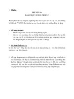
Figure 5-1. POS tagged data from four Indian languages: Bangla, Hindi, Marathi, and Telugu.
Let’s see which of these tags are the most common in the news category of the Brown

Corpus:
>>> from nltk.corpus import brown
>>> brown_news_tagged = brown.tagged_words(categories='news', simplify_tags=True)
>>> tag_fd = nltk.FreqDist(tag for (word, tag) in brown_news_tagged)
>>> tag_fd.keys()
['N', 'P', 'DET', 'NP', 'V', 'ADJ', ',', '.', 'CNJ', 'PRO', 'ADV', 'VD', ]
Your Turn: Plot the frequency distribution just shown using
tag_fd.plot(cumulative=True). What percentage of words are tagged
using the first five tags of the above list?
We can use these tags to do powerful searches using a graphical POS-concordance tool
nltk.app.concordance(). Use it to search for any combination of words and POS tags,
e.g., N N N N, hit/VD, hit/VN, or the ADJ man.
Nouns
Nouns generally refer to people, places, things, or concepts, e.g., woman, Scotland,
book, intelligence. Nouns can appear after determiners and adjectives, and can be the
subject or object of the verb, as shown in Table 5-2.
Table 5-2. Syntactic patterns involving some nouns
Word After a determiner Subject of the verb
woman the woman who I saw yesterday the woman sat down
Scotland the Scotland I remember as a child Scotland has five million people
book the book I bought yesterday this book recounts the colonization of Australia
intelligence the intelligence displayed by the child Mary’s intelligence impressed her teachers
The simplified noun tags are N for
common nouns like book, and NP for proper nouns
like Scotland.
184 | Chapter 5: Categorizing and Tagging Words
Let’s inspect some tagged text to see what parts-of-speech occur before a noun, with
the most frequent ones first. To begin with, we construct a list of bigrams whose mem-
bers are themselves word-tag pairs, such as (('The', 'DET'), ('Fulton', 'NP')) and
(('Fulton', 'NP'), ('County', 'N')). Then we construct a FreqDist from the tag parts

of the bigrams.
>>> word_tag_pairs = nltk.bigrams(brown_news_tagged)
>>> list(nltk.FreqDist(a[1] for (a, b) in word_tag_pairs if b[1] == 'N'))
['DET', 'ADJ', 'N', 'P', 'NP', 'NUM', 'V', 'PRO', 'CNJ', '.', ',', 'VG', 'VN', ]
This confirms our assertion that nouns occur after determiners and adjectives, includ-
ing numeral adjectives (tagged as NUM).
Verbs
Verbs are words that describe events and actions, e.g., fall and eat, as shown in Ta-
ble 5-3. In the context of a sentence, verbs typically express a relation involving the
referents of one or more noun phrases.
Table 5-3. Syntactic patterns involving some verbs
Word Simple With modifiers and adjuncts (italicized)
fall Rome fell Dot com stocks suddenly fell like a stone
eat Mice eat cheese John ate the pizza with gusto
What are the most common verbs in news text? Let’s sort all the verbs by frequency:
>>> wsj = nltk.corpus.treebank.tagged_words(simplify_tags=True)
>>> word_tag_fd = nltk.FreqDist(wsj)
>>> [word + "/" + tag for (word, tag) in word_tag_fd if tag.startswith('V')]
['is/V', 'said/VD', 'was/VD', 'are/V', 'be/V', 'has/V', 'have/V', 'says/V',
'were/VD', 'had/VD', 'been/VN', "'s/V", 'do/V', 'say/V', 'make/V', 'did/VD',
'rose/VD', 'does/V', 'expected/VN', 'buy/V', 'take/V', 'get/V', 'sell/V',
'help/V', 'added/VD', 'including/VG', 'according/VG', 'made/VN', 'pay/V', ]
Note
that
the items being counted in the frequency distribution are word-tag pairs.
Since words and tags are paired, we can treat the word as a condition and the tag as an
event, and initialize a conditional frequency distribution with a list of condition-event
pairs. This lets us see a frequency-ordered list of tags given a word:
>>> cfd1 = nltk.ConditionalFreqDist(wsj)
>>> cfd1['yield'].keys()

['V', 'N']
>>> cfd1['cut'].keys()
['V', 'VD', 'N', 'VN']
We can reverse the order of the pairs, so that the tags are the conditions, and the words
are the events. Now we can see likely words for a given tag:
5.2 Tagged Corpora | 185
>>> cfd2 = nltk.ConditionalFreqDist((tag, word) for (word, tag) in wsj)
>>> cfd2['VN'].keys()
['been', 'expected', 'made', 'compared', 'based', 'priced', 'used', 'sold',
'named', 'designed', 'held', 'fined', 'taken', 'paid', 'traded', 'said', ]
To
clarify
the distinction between VD (past tense) and VN (past participle), let’s find
words that can be both VD and VN, and see some surrounding text:
>>> [w for w in cfd1.conditions() if 'VD' in cfd1[w] and 'VN' in cfd1[w]]
['Asked', 'accelerated', 'accepted', 'accused', 'acquired', 'added', 'adopted', ]
>>> idx1 = wsj.index(('kicked', 'VD'))
>>> wsj[idx1-4:idx1+1]
[('While', 'P'), ('program', 'N'), ('trades', 'N'), ('swiftly', 'ADV'),
('kicked', 'VD')]
>>> idx2 = wsj.index(('kicked', 'VN'))
>>> wsj[idx2-4:idx2+1]
[('head', 'N'), ('of', 'P'), ('state', 'N'), ('has', 'V'), ('kicked', 'VN')]
In this case, we see that the past participle of kicked is preceded by a form of the auxiliary
verb have. Is this generally true?
Your Turn: Given
the list of past participles specified by
cfd2['VN'].keys(), try to collect a list of all the word-tag pairs that im-
mediately precede items in that list.
Adjectives and Adverbs

Two other important word classes are adjectives and adverbs. Adjectives describe
nouns, and can be used as modifiers (e.g., large in the large pizza), or as predicates (e.g.,
the pizza is large). English adjectives can have internal structure (e.g., fall+ing in the
falling stocks). Adverbs modify verbs to specify the time, manner, place, or direction of
the event described by the verb (e.g., quickly in the stocks fell quickly). Adverbs may
also modify adjectives (e.g., really in Mary’s teacher was really nice).
English has several categories of closed class words in addition to prepositions, such
as articles (also often called determiners) (e.g., the, a), modals (e.g., should, may),
and personal pronouns (e.g., she, they). Each dictionary and grammar classifies these
words differently.
Your Turn: If you are uncertain about some of these parts-of-speech,
study them using nltk.app.concordance(), or watch some of the School-
house Rock! grammar videos available at YouTube, or consult Sec-
tion 5.9.
186 | Chapter 5: Categorizing and Tagging Words
Unsimplified Tags
Let’s find the most frequent nouns of each noun part-of-speech type. The program in
Example 5-1 finds all tags starting with NN, and provides a few example words for each
one. You will see that there are many variants of NN; the most important contain $ for
possessive nouns, S for plural nouns (since plural nouns typically end in s), and P for
proper nouns. In addition, most of the tags have suffix modifiers: -NC for citations,
-HL for words in headlines, and -TL for titles (a feature of Brown tags).
Example 5-1. Program to find the most frequent noun tags.
def findtags(tag_prefix, tagged_text):
cfd = nltk.ConditionalFreqDist((tag, word) for (word, tag) in tagged_text
if tag.startswith(tag_prefix))
return dict((tag, cfd[tag].keys()[:5]) for tag in cfd.conditions())
>>> tagdict = findtags('NN', nltk.corpus.brown.tagged_words(categories='news'))
>>> for tag in sorted(tagdict):
print tag, tagdict[tag]

NN ['year', 'time', 'state', 'week', 'man']
NN$ ["year's", "world's", "state's", "nation's", "company's"]
NN$-HL ["Golf's", "Navy's"]
NN$-TL ["President's", "University's", "League's", "Gallery's", "Army's"]
NN-HL ['cut', 'Salary', 'condition', 'Question', 'business']
NN-NC ['eva', 'ova', 'aya']
NN-TL ['President', 'House', 'State', 'University', 'City']
NN-TL-HL ['Fort', 'City', 'Commissioner', 'Grove', 'House']
NNS ['years', 'members', 'people', 'sales', 'men']
NNS$ ["children's", "women's", "men's", "janitors'", "taxpayers'"]
NNS$-HL ["Dealers'", "Idols'"]
NNS$-TL ["Women's", "States'", "Giants'", "Officers'", "Bombers'"]
NNS-HL ['years', 'idols', 'Creations', 'thanks', 'centers']
NNS-TL ['States', 'Nations', 'Masters', 'Rules', 'Communists']
NNS-TL-HL ['Nations']
When
we come to constructing part-of-speech taggers later in this chapter, we will use
the unsimplified tags.
Exploring Tagged Corpora
Let’s briefly return to the kinds of exploration of corpora we saw in previous chapters,
this time exploiting POS tags.
Suppose we’re studying the word often and want to see how it is used in text. We could
ask to see the words that follow often:
>>> brown_learned_text = brown.words(categories='learned')
>>> sorted(set(b for (a, b) in nltk.ibigrams(brown_learned_text) if a == 'often'))
[',', '.', 'accomplished', 'analytically', 'appear', 'apt', 'associated', 'assuming',
'became', 'become', 'been', 'began', 'call', 'called', 'carefully', 'chose', ]
However, it’s probably more instructive use the tagged_words() method to look at the
part-of-speech tag of the following words:

5.2 Tagged Corpora | 187
>>> brown_lrnd_tagged = brown.tagged_words(categories='learned', simplify_tags=True)
>>> tags = [b[1] for (a, b) in nltk.ibigrams(brown_lrnd_tagged) if a[0] == 'often']
>>> fd = nltk.FreqDist(tags)
>>> fd.tabulate()
VN V VD DET ADJ ADV P CNJ , TO VG WH VBZ .
15 12 8 5 5 4 4 3 3 1 1 1 1 1
Notice that the most high-frequency parts-of-speech following often are verbs. Nouns
never appear in this position (in this particular corpus).
Next,
let’s
look at some larger context, and find words involving particular sequences
of tags and words (in this case "<Verb> to <Verb>"). In Example 5-2, we consider each
three-word window in the sentence
, and check whether they meet our criterion .
If the tags match, we print the corresponding words .
Example 5-2. Searching for three-word phrases using POS tags.
from nltk.corpus import brown
def process(sentence):
for (w1,t1), (w2,t2), (w3,t3) in nltk.trigrams(sentence):
if (t1.startswith('V') and t2 == 'TO' and t3.startswith('V')):
print w1, w2, w3
>>> for tagged_sent in brown.tagged_sents():
process(tagged_sent)

combined to achieve
continue to place
serve to protect
wanted to wait
allowed to place

expected to become

Finally,
let’s
look for words that are highly ambiguous as to their part-of-speech tag.
Understanding why such words are tagged as they are in each context can help us clarify
the distinctions between the tags.
>>> brown_news_tagged = brown.tagged_words(categories='news', simplify_tags=True)
>>> data = nltk.ConditionalFreqDist((word.lower(), tag)
for (word, tag) in brown_news_tagged)
>>> for word in data.conditions():
if len(data[word]) > 3:
tags = data[word].keys()
print word, ' '.join(tags)

best ADJ ADV NP V
better ADJ ADV V DET
close ADV ADJ V N
cut V N VN VD
even ADV DET ADJ V
grant NP N V -
hit V VD VN N
lay ADJ V NP VD
left VD ADJ N VN
188 | Chapter 5: Categorizing and Tagging Words
like CNJ V ADJ P -
near P ADV ADJ DET
open ADJ V N ADV
past N ADJ DET P
present ADJ ADV V N

read V VN VD NP
right ADJ N DET ADV
second NUM ADV DET N
set VN V VD N -
that CNJ V WH DET
Your Turn: Open
the POS concordance tool nltk.app.concordance()
and load the complete Brown Corpus (simplified tagset). Now pick
some of the words listed at the end of the previous code example and
see how the tag of the word correlates with the context of the word. E.g.,
search for near to see all forms mixed together, near/ADJ to see it used
as an adjective, near N to see just those cases where a noun follows, and
so forth.
5.3 Mapping Words to Properties Using Python Dictionaries
As we have seen, a tagged word of the form (word, tag) is an association between a
word and a part-of-speech tag. Once we start doing part-of-speech tagging, we will be
creating programs that assign a tag to a word, the tag which is most likely in a given
context. We can think of this process as mapping from words to tags. The most natural
way to store mappings in Python uses the so-called dictionary data type (also known
as an associative array or hash array in other programming languages). In this sec-
tion, we look at dictionaries and see how they can represent a variety of language in-
formation, including parts-of-speech.
Indexing Lists Versus Dictionaries
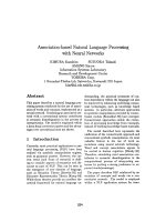
A text, as we have seen, is treated in Python as a list of words. An important property
of lists is that we can “look up” a particular item by giving its index, e.g., text1[100].
Notice how we specify a number and get back a word. We can think of a list as a simple
kind of table, as shown in Figure 5-2.
Figure 5-2. List lookup: We access the contents of a Python list with the help of an integer index.
5.3 Mapping Words to Properties Using Python Dictionaries | 189
Contrast this situation with frequency distributions (Section 1.3), where we specify a

word and get back a number, e.g., fdist['monstrous'], which tells us the number of
times a given word has occurred in a text. Lookup using words is familiar to anyone
who has used a dictionary. Some more examples are shown in Figure 5-3.
Figure 5-3. Dictionary lookup: we access the entry of a dictionary using a key such as someone’s name,
a web
domain, or an English word; other names for dictionary are map, hashmap, hash, and
associative array.
In the case of a phonebook, we look up an entry using a name and get back a number.
When we type a domain name in a web browser, the computer looks this up to get
back an IP address. A word frequency table allows us to look up a word and find its
frequency in a text collection. In all these cases, we are mapping from names to num-
bers, rather than the other way around as with a list. In general, we would like to be
able to map between arbitrary types of information. Table 5-4 lists a variety of linguistic
objects, along with what they map.
Table 5-4. Linguistic objects as mappings from keys to values
Linguistic object Maps from Maps to
Document Index Word List of pages (where word is found)
Thesaurus Word sense List of synonyms
Dictionary Headword Entry (part-of-speech, sense definitions, etymology)
Comparative Wordlist Gloss term Cognates (list of words, one per language)
Morph Analyzer Surface form Morphological analysis (list of component morphemes)
Most often, we are mapping from a “word” to some structured object. For example, a
document index maps from a word (which we can represent as a string) to a list of pages
(represented as a list of integers). In this section, we will see how to represent such
mappings in Python.
Dictionaries in Python
Python provides a dictionary data type that can be used for mapping between arbitrary
types. It is like a conventional dictionary, in that it gives you an efficient way to look
things up. However, as we see from Table 5-4, it has a much wider range of uses.
190 | Chapter 5: Categorizing and Tagging Words

To illustrate, we define pos to be an empty dictionary and then add four entries to it,
specifying the part-of-speech of some words. We add entries to a dictionary using the
familiar square bracket notation:
>>> pos = {}
>>> pos
{}
>>> pos['colorless'] = 'ADJ'
>>> pos
{'colorless': 'ADJ'}
>>> pos['ideas'] = 'N'
>>> pos['sleep'] = 'V'
>>> pos['furiously'] = 'ADV'
>>> pos
{'furiously': 'ADV', 'ideas': 'N', 'colorless': 'ADJ', 'sleep': 'V'}
So, for
example,
says that the part-of-speech of colorless is
adjective, or more spe-
cifically, that the key 'colorless' is assigned the value 'ADJ' in dictionary pos. When
we inspect the value of pos
we see a set of key-value pairs. Once we have populated
the dictionary in this way, we can employ the keys to retrieve values:
>>> pos['ideas']
'N'
>>> pos['colorless']
'ADJ'
Of course, we might accidentally use a key that hasn’t been assigned a value.
>>> pos['green']
Traceback (most recent call last):
File "<stdin>", line 1, in ?

KeyError: 'green'
This
raises
an important question. Unlike lists and strings, where we can use len() to
work out which integers will be legal indexes, how do we work out the legal keys for a
dictionary? If the dictionary is not too big, we can simply inspect its contents by eval-
uating the variable pos. As we saw earlier in line
, this gives us the key-value pairs.
Notice that
they are not in the same order they were originally entered; this is because
dictionaries are not sequences but mappings (see Figure 5-3), and the keys are not
inherently ordered.
Alternatively, to just find the keys, we can either convert the dictionary to a list
or
use the dictionary in a context where a list is expected, as the parameter of sorted()
or in a for loop .
>>> list(pos)
['ideas', 'furiously', 'colorless', 'sleep']
>>> sorted(pos)
['colorless', 'furiously', 'ideas', 'sleep']
>>> [w for w in pos if w.endswith('s')]
['colorless', 'ideas']
5.3 Mapping Words to Properties Using Python Dictionaries | 191
When you type list(pos), you might see a different order to the one
shown here. If you want to see the keys in order, just sort them.
As well as iterating over all keys in the dictionary with a for loop, we can use the for
loop as we did for printing lists:
>>> for word in sorted(pos):
print word + ":", pos[word]

colorless: ADJ
furiously: ADV
sleep: V
ideas: N
Finally, the dictionary methods keys(), values(), and items() allow us to access the
keys, values, and key-value pairs as separate lists. We can even sort tuples
, which
orders them
according to their first element (and if the first elements are the same, it
uses their second elements).
>>> pos.keys()
['colorless', 'furiously', 'sleep', 'ideas']
>>> pos.values()
['ADJ', 'ADV', 'V', 'N']
>>> pos.items()
[('colorless', 'ADJ'), ('furiously', 'ADV'), ('sleep', 'V'), ('ideas', 'N')]
>>> for key, val in sorted(pos.items()):
print key + ":", val

colorless: ADJ
furiously: ADV
ideas: N
sleep: V
We
want
to be sure that when we look something up in a dictionary, we get only one
value for each key. Now suppose we try to use a dictionary to store the fact that the
word sleep can be used as both a verb and a noun:
>>> pos['sleep'] = 'V'
>>> pos['sleep']

'V'
>>> pos['sleep'] = 'N'
>>> pos['sleep']
'N'
Initially, pos['sleep'] is given the value 'V'. But this is immediately overwritten with
the new value, 'N'. In other words, there can be only one entry in the dictionary for
'sleep'. However, there is a way of storing multiple values in that entry: we use a list
value, e.g., pos['sleep'] = ['N', 'V']. In fact, this is what we saw in Section 2.4 for
the CMU Pronouncing Dictionary, which stores multiple pronunciations for a single
word.
192 | Chapter 5: Categorizing and Tagging Words
Defining Dictionaries
We can use the same key-value pair format to create a dictionary. There are a couple
of ways to do this, and we will normally use the first:
>>> pos = {'colorless': 'ADJ', 'ideas': 'N', 'sleep': 'V', 'furiously': 'ADV'}
>>> pos = dict(colorless='ADJ', ideas='N', sleep='V', furiously='ADV')
Note that dictionary keys must be immutable types, such as strings and tuples. If we
try to define a dictionary using a mutable key, we get a TypeError:
>>> pos = {['ideas', 'blogs', 'adventures']: 'N'}
Traceback (most recent call last):
File "<stdin>", line 1, in <module>
TypeError: list objects are unhashable
Default Dictionaries
If we try to access a key that is not in a dictionary, we get an error. However, it’s often
useful if a dictionary can automatically create an entry for this new key and give it a
default value, such as zero or the empty list. Since Python 2.5, a special kind of dic-
tionary called a defaultdict has been available. (It is provided as nltk.defaultdict for
the benefit of readers who are using Python 2.4.) In order to use it, we have to supply
a parameter which can be used to create the default value, e.g., int, float, str, list,
dict, tuple.

>>> frequency = nltk.defaultdict(int)
>>> frequency['colorless'] = 4
>>> frequency['ideas']
0
>>> pos = nltk.defaultdict(list)
>>> pos['sleep'] = ['N', 'V']
>>> pos['ideas']
[]
These default values are actually functions that convert other objects to
the specified
type (e.g., int("2"), list("2")). When they are called with
no parameter—say, int(), list()—they return 0 and [] respectively.
The preceding examples specified the default value of a dictionary entry to be the default
value of a particular data type. However, we can specify any default value we like, simply
by providing the name of a function that can be called with no arguments to create the
required value. Let’s return to our part-of-speech example, and create a dictionary
whose default value for any entry is 'N'
. When we access a non-existent entry , it
is automatically added to the dictionary .
>>> pos = nltk.defaultdict(lambda: 'N')
>>> pos['colorless'] = 'ADJ'
>>> pos['blog']
'N'
5.3 Mapping Words to Properties Using Python Dictionaries | 193
>>> pos.items()
[('blog', 'N'), ('colorless', 'ADJ')]
This example used a lambda expression
, introduced in Section 4.4. This
lambda expression specifies no parameters, so we call it using paren-
theses with no arguments. Thus, the following definitions of f and g are

equivalent:
>>> f = lambda: 'N'
>>> f()
'N'
>>> def g():
return 'N'
>>> g()
'N'
Let’s
see
how default dictionaries could be used in a more substantial language pro-
cessing task. Many language processing tasks—including tagging—struggle to cor-
rectly process the hapaxes of a text. They can perform better with a fixed vocabulary
and a guarantee that no new words will appear. We can preprocess a text to replace
low-frequency words with a special “out of vocabulary” token, UNK, with the help of a
default dictionary. (Can you work out how to do this without reading on?)
We need to create a default dictionary that maps each word to its replacement. The
most frequent n words will be mapped to themselves. Everything else will be mapped
to UNK.
>>> alice = nltk.corpus.gutenberg.words('carroll-alice.txt')
>>> vocab = nltk.FreqDist(alice)
>>> v1000 = list(vocab)[:1000]
>>> mapping = nltk.defaultdict(lambda: 'UNK')
>>> for v in v1000:
mapping[v] = v

>>> alice2 = [mapping[v] for v in alice]
>>> alice2[:100]
['UNK', 'Alice', "'", 's', 'Adventures', 'in', 'Wonderland', 'by', 'UNK', 'UNK',
'UNK', 'UNK', 'CHAPTER', 'I', '.', 'UNK', 'the', 'Rabbit', '-', 'UNK', 'Alice',

'was', 'beginning', 'to', 'get', 'very', 'tired', 'of', 'sitting', 'by', 'her',
'sister', 'on', 'the', 'bank', ',', 'and', 'of', 'having', 'nothing', 'to', 'do',
':', 'once', 'or', 'twice', 'she', 'had', 'UNK', 'into', 'the', 'book', 'her',
'sister', 'was', 'UNK', ',', 'but', 'it', 'had', 'no', 'pictures', 'or', 'UNK',
'in', 'it', ',', "'", 'and', 'what', 'is', 'the', 'use', 'of', 'a', 'book', ",'",
'thought', 'Alice', "'", 'without', 'pictures', 'or', 'conversation', "?'", ]
>>> len(set(alice2))
1001
Incrementally Updating a Dictionary
We can employ dictionaries to count occurrences, emulating the method for tallying
words shown in Figure 1-3. We begin by initializing an empty defaultdict, then process
each part-of-speech tag in the text. If the tag hasn’t been seen before, it will have a zero
194 | Chapter 5: Categorizing and Tagging Words
count by default. Each time we encounter a tag, we increment its count using the +=
operator (see Example 5-3).
Example 5-3. Incrementally updating a dictionary, and sorting by value.
>>> counts = nltk.defaultdict(int)
>>> from nltk.corpus import brown
>>> for (word, tag) in brown.tagged_words(categories='news'):
counts[tag] += 1

>>> counts['N']
22226
>>> list(counts)
['FW', 'DET', 'WH', "''", 'VBZ', 'VB+PPO', "'", ')', 'ADJ', 'PRO', '*', '-', ]
>>> from operator import itemgetter
>>> sorted(counts.items(), key=itemgetter(1), reverse=True)
[('N', 22226), ('P', 10845), ('DET', 10648), ('NP', 8336), ('V', 7313), ]
>>> [t for t, c in sorted(counts.items(), key=itemgetter(1), reverse=True)]
['N', 'P', 'DET', 'NP', 'V', 'ADJ', ',', '.', 'CNJ', 'PRO', 'ADV', 'VD', ]

The
listing in Example 5-3 illustrates an important idiom for sorting a dictionary by its
values, to show words in decreasing order of frequency. The first parameter of
sorted() is the items to sort, which is a list of tuples consisting of a POS tag and a
frequency. The second parameter specifies the sort key using a function itemget
ter(). In general, itemgetter(n) returns a function that can be called on some other
sequence object to obtain the nth element:
>>> pair = ('NP', 8336)
>>> pair[1]
8336
>>> itemgetter(1)(pair)
8336
The last parameter of sorted() specifies that the items should be returned in reverse
order, i.e., decreasing values of frequency.
There’s a second useful programming idiom at the beginning of Example 5-3, where
we initialize a defaultdict and then use a for loop to update its values. Here’s a sche-
matic version:
>>> my_dictionary = nltk.defaultdict(function to create default value)
>>> for item in sequence:
my_dictionary[item_key] is updated with information about item
Here’s another instance of this pattern, where we index words according to their last
two letters:
>>> last_letters = nltk.defaultdict(list)
>>> words = nltk.corpus.words.words('en')
>>> for word in words:
key = word[-2:]
last_letters[key].append(word)

5.3 Mapping Words to Properties Using Python Dictionaries | 195
>>> last_letters['ly']

['abactinally', 'abandonedly', 'abasedly', 'abashedly', 'abashlessly', 'abbreviately',
'abdominally', 'abhorrently', 'abidingly', 'abiogenetically', 'abiologically', ]
>>> last_letters['zy']
['blazy', 'bleezy', 'blowzy', 'boozy', 'breezy', 'bronzy', 'buzzy', 'Chazy', ]
The
following
example uses the same pattern to create an anagram dictionary. (You
might experiment with the third line to get an idea of why this program works.)
>>> anagrams = nltk.defaultdict(list)
>>> for word in words:
key = ''.join(sorted(word))
anagrams[key].append(word)

>>> anagrams['aeilnrt']
['entrail', 'latrine', 'ratline', 'reliant', 'retinal', 'trenail']
Since accumulating words like this is such a common task, NLTK provides a more
convenient way of creating a defaultdict(list), in the form of nltk.Index():
>>> anagrams = nltk.Index((''.join(sorted(w)), w) for w in words)
>>> anagrams['aeilnrt']
['entrail', 'latrine', 'ratline', 'reliant', 'retinal', 'trenail']
nltk.Index is a defaultdict(list) with extra support for initialization.
Similarly, nltk.FreqDist
is
essentially a defaultdict(int) with extra
support for initialization (along with sorting and plotting methods).
Complex Keys and Values
We can use default dictionaries with complex keys and values. Let’s study the range of
possible tags for a word, given the word itself and the tag of the previous word. We will
see how this information can be used by a POS tagger.
>>> pos = nltk.defaultdict(lambda: nltk.defaultdict(int))

>>> brown_news_tagged = brown.tagged_words(categories='news', simplify_tags=True)
>>> for ((w1, t1), (w2, t2)) in nltk.ibigrams(brown_news_tagged):
pos[(t1, w2)][t2] += 1

>>> pos[('DET', 'right')]
defaultdict(<type 'int'>, {'ADV': 3, 'ADJ': 9, 'N': 3})
This
example
uses a dictionary whose default value for an entry is a dictionary (whose
default value is int(), i.e., zero). Notice how we iterated over the bigrams of the tagged
corpus, processing a pair of word-tag pairs for each iteration
. Each time through the
loop
we
updated our pos dictionary’s entry for (t1, w2), a tag and its following word
. When we look up an item in pos
we
must specify a compound key
, and we get
back
a
dictionary object. A POS tagger could use such information to decide that the
word right, when preceded by a determiner, should be tagged as ADJ.
196 | Chapter 5: Categorizing and Tagging Words
Inverting a Dictionary
Dictionaries support efficient lookup, so long as you want to get the value for any key.
If d is a dictionary and k is a key, we type d[k] and immediately obtain the value. Finding
a key given a value is slower and more cumbersome:
>>> counts = nltk.defaultdict(int)
>>> for word in nltk.corpus.gutenberg.words('milton-paradise.txt'):

counts[word] += 1

>>> [key for (key, value) in counts.items() if value == 32]
['brought', 'Him', 'virtue', 'Against', 'There', 'thine', 'King', 'mortal',
'every', 'been']
If we expect to do this kind of “reverse lookup” often, it helps to construct a dictionary
that maps values to keys. In the case that no two keys have the same value, this is an
easy thing to do. We just get all the key-value pairs in the dictionary, and create a new
dictionary of value-key pairs. The next example also illustrates another way of initial-
izing a dictionary pos with key-value pairs.
>>> pos = {'colorless': 'ADJ', 'ideas': 'N', 'sleep': 'V', 'furiously': 'ADV'}
>>> pos2 = dict((value, key) for (key, value) in pos.items())
>>> pos2['N']
'ideas'
Let’s first make our part-of-speech dictionary a bit more realistic and add some more
words to pos using the dictionary update() method, to create the situation where mul-
tiple keys have the same value. Then the technique just shown for reverse lookup will
no longer work (why not?). Instead, we have to use append() to accumulate the words
for each part-of-speech, as follows:
>>> pos.update({'cats': 'N', 'scratch': 'V', 'peacefully': 'ADV', 'old': 'ADJ'})
>>> pos2 = nltk.defaultdict(list)
>>> for key, value in pos.items():
pos2[value].append(key)

>>> pos2['ADV']
['peacefully', 'furiously']
Now we have inverted the pos dictionary, and can look up any part-of-speech and find
all words having that part-of-speech. We can do the same thing even more simply using
NLTK’s support for indexing, as follows:
>>> pos2 = nltk.Index((value, key) for (key, value) in pos.items())

>>> pos2['ADV']
['peacefully', 'furiously']
A summary of Python’s dictionary methods is given in Table 5-5.
5.3 Mapping Words to Properties Using Python Dictionaries | 197
Table 5-5. Python’s dictionary methods: A summary of commonly used methods and idioms involving
dictionaries
Example Description
d = {} Create an empty dictionary and assign it to d
d[key] = value Assign a value to a given dictionary key
d.keys() The list of keys of the dictionary
list(d) The list of keys of the dictionary
sorted(d) The keys of the dictionary, sorted
key in d Test whether a particular key is in the dictionary
for key in d Iterate over the keys of the dictionary
d.values() The list of values in the dictionary
dict([(k1,v1), (k2,v2), ]) Create a dictionary from a list of key-value pairs
d1.update(d2) Add all items from d2 to d1
defaultdict(int) A dictionary whose default value is zero
5.4 Automatic Tagging
In the rest of this chapter we will explore various ways to automatically add part-of-
speech tags to text. We will see that the tag of a word depends on the word and its
context within a sentence. For this reason, we will be working with data at the level of
(tagged) sentences rather than words. We’ll begin by loading the data we will be using.
>>> from nltk.corpus import brown
>>> brown_tagged_sents = brown.tagged_sents(categories='news')
>>> brown_sents = brown.sents(categories='news')
The Default Tagger
The simplest possible tagger assigns the same tag to each token. This may seem to be
a rather banal step, but it establishes an important baseline for tagger performance. In
order to get the best result, we tag each word with the most likely tag. Let’s find out

which tag is most likely (now using the unsimplified tagset):
>>> tags = [tag for (word, tag) in brown.tagged_words(categories='news')]
>>> nltk.FreqDist(tags).max()
'NN'
Now we can create a tagger that tags everything as NN.
>>> raw = 'I do not like green eggs and ham, I do not like them Sam I am!'
>>> tokens = nltk.word_tokenize(raw)
>>> default_tagger = nltk.DefaultTagger('NN')
>>> default_tagger.tag(tokens)
[('I', 'NN'), ('do', 'NN'), ('not', 'NN'), ('like', 'NN'), ('green', 'NN'),
('eggs', 'NN'), ('and', 'NN'), ('ham', 'NN'), (',', 'NN'), ('I', 'NN'),
198 | Chapter 5: Categorizing and Tagging Words
('do', 'NN'), ('not', 'NN'), ('like', 'NN'), ('them', 'NN'), ('Sam', 'NN'),
('I', 'NN'), ('am', 'NN'), ('!', 'NN')]
Unsurprisingly, this
method performs rather poorly. On a typical corpus, it will tag
only about an eighth of the tokens correctly, as we see here:
>>> default_tagger.evaluate(brown_tagged_sents)
0.13089484257215028
Default taggers assign their tag to every single word, even words that have never been
encountered before. As it happens, once we have processed several thousand words of
English text, most new words will be nouns. As we will see, this means that default
taggers can help to improve the robustness of a language processing system. We will
return to them shortly.
The Regular Expression Tagger
The regular expression tagger assigns tags to tokens on the basis of matching patterns.
For instance, we might guess that any word ending in ed is the past participle of a verb,
and any word ending with ’s is a possessive noun. We can express these as a list of
regular expressions:
>>> patterns = [

(r'.*ing$', 'VBG'), # gerunds
(r'.*ed$', 'VBD'), # simple past
(r'.*es$', 'VBZ'), # 3rd singular present
(r'.*ould$', 'MD'), # modals
(r'.*\'s$', 'NN$'), # possessive nouns
(r'.*s$', 'NNS'), # plural nouns
(r'^-?[0-9]+(.[0-9]+)?$', 'CD'), # cardinal numbers
(r'.*', 'NN') # nouns (default)
]
Note that these are processed in order, and the first one that matches is applied. Now
we can set up a tagger and use it to tag a sentence. After this step, it is correct about a
fifth of the time.
>>> regexp_tagger = nltk.RegexpTagger(patterns)
>>> regexp_tagger.tag(brown_sents[3])
[('``', 'NN'), ('Only', 'NN'), ('a', 'NN'), ('relative', 'NN'), ('handful', 'NN'),
('of', 'NN'), ('such', 'NN'), ('reports', 'NNS'), ('was', 'NNS'), ('received', 'VBD'),
("''", 'NN'), (',', 'NN'), ('the', 'NN'), ('jury', 'NN'), ('said', 'NN'), (',', 'NN'),
('``', 'NN'), ('considering', 'VBG'), ('the', 'NN'), ('widespread', 'NN'), ]
>>> regexp_tagger.evaluate(brown_tagged_sents)
0.20326391789486245
The final regular expression «.*» is a catch-all that tags everything as a noun. This is
equivalent to the default tagger (only much less efficient). Instead of respecifying this
as part of the regular expression tagger, is there a way to combine this tagger with the
default tagger? We will see how to do this shortly.
5.4 Automatic Tagging | 199
Your Turn: See if you can come up with patterns to improve the per-
formance of the regular expression tagger just shown. (Note that Sec-
tion 6.1 describes a way to partially automate such work.)
The Lookup Tagger
A lot of high-frequency words do not have the NN tag. Let’s find the hundred most

frequent words and store their most likely tag. We can then use this information as the
model for a “lookup tagger” (an NLTK UnigramTagger):
>>> fd = nltk.FreqDist(brown.words(categories='news'))
>>> cfd = nltk.ConditionalFreqDist(brown.tagged_words(categories='news'))
>>> most_freq_words = fd.keys()[:100]
>>> likely_tags = dict((word, cfd[word].max()) for word in most_freq_words)
>>> baseline_tagger = nltk.UnigramTagger(model=likely_tags)
>>> baseline_tagger.evaluate(brown_tagged_sents)
0.45578495136941344
It should come as no surprise by now that simply knowing the tags for the 100 most
frequent words enables us to tag a large fraction of tokens correctly (nearly half, in fact).
Let’s see what it does on some untagged input text:
>>> sent = brown.sents(categories='news')[3]
>>> baseline_tagger.tag(sent)
[('``', '``'), ('Only', None), ('a', 'AT'), ('relative', None),
('handful', None), ('of', 'IN'), ('such', None), ('reports', None),
('was', 'BEDZ'), ('received', None), ("''", "''"), (',', ','),
('the', 'AT'), ('jury', None), ('said', 'VBD'), (',', ','),
('``', '``'), ('considering', None), ('the', 'AT'), ('widespread', None),
('interest', None), ('in', 'IN'), ('the', 'AT'), ('election', None),
(',', ','), ('the', 'AT'), ('number', None), ('of', 'IN'),
('voters', None), ('and', 'CC'), ('the', 'AT'), ('size', None),
('of', 'IN'), ('this', 'DT'), ('city', None), ("''", "''"), ('.', '.')]
Many words have been assigned a tag of None, because they were not among the 100
most frequent words. In these cases we would like to assign the default tag of NN. In
other words, we want to use the lookup table first, and if it is unable to assign a tag,
then use the default tagger, a process known as backoff (Section 5.5). We do this by
specifying one tagger as a parameter to the other, as shown next. Now the lookup tagger
will only store word-tag pairs for words other than nouns, and whenever it cannot
assign a tag to a word, it will invoke the default tagger.

>>> baseline_tagger = nltk.UnigramTagger(model=likely_tags,
backoff=nltk.DefaultTagger('NN'))
Let’s put all this together and write a program to create and evaluate lookup taggers
having a range of sizes (Example 5-4).
200 | Chapter 5: Categorizing and Tagging Words
Example 5-4. Lookup tagger performance with varying model size.
def performance(cfd, wordlist):
lt = dict((word, cfd[word].max()) for word in wordlist)
baseline_tagger = nltk.UnigramTagger(model=lt, backoff=nltk.DefaultTagger('NN'))
return baseline_tagger.evaluate(brown.tagged_sents(categories='news'))
def display():
import pylab
words_by_freq = list(nltk.FreqDist(brown.words(categories='news')))
cfd = nltk.ConditionalFreqDist(brown.tagged_words(categories='news'))
sizes = 2 ** pylab.arange(15)
perfs = [performance(cfd, words_by_freq[:size]) for size in sizes]
pylab.plot(sizes, perfs, '-bo')
pylab.title('Lookup Tagger Performance with Varying Model Size')
pylab.xlabel('Model Size')
pylab.ylabel('Performance')
pylab.show()
>>> display()
Observe
in Figure 5-4 that performance initially increases rapidly as the model size
grows, eventually reaching a plateau, when large increases in model size yield little
improvement in performance. (This example used the pylab plotting package, dis-
cussed in Section 4.8.)
Evaluation
In the previous examples, you will have noticed an emphasis on accuracy scores. In
fact, evaluating the performance of such tools is a central theme in NLP. Recall the

processing pipeline in Figure 1-5; any errors in the output of one module are greatly
multiplied in the downstream modules.
We evaluate the performance of a tagger relative to the tags a human expert would
assign. Since we usually don’t have access to an expert and impartial human judge, we
make do instead with gold standard test data. This is a corpus which has been man-
ually annotated and accepted as a standard against which the guesses of an automatic
system are assessed. The tagger is regarded as being correct if the tag it guesses for a
given word is the same as the gold standard tag.
Of course, the humans who designed and carried out the original gold standard anno-
tation were only human. Further analysis might show mistakes in the gold standard,
or may eventually lead to a revised tagset and more elaborate guidelines. Nevertheless,
the gold standard is by definition “correct” as far as the evaluation of an automatic
tagger is concerned.
5.4 Automatic Tagging | 201
Developing an annotated corpus is a major undertaking. Apart from the
data, it
generates sophisticated tools, documentation, and practices for
ensuring high-quality annotation. The tagsets and other coding schemes
inevitably depend on some theoretical position that is not shared by all.
However, corpus creators often go to great lengths to make their work
as theory-neutral as possible in order to maximize the usefulness of their
work. We will discuss the challenges of creating a corpus in Chapter 11.
5.5 N-Gram Tagging
Unigram Tagging
Unigram taggers are based on a simple statistical algorithm: for each token, assign the
tag that is most likely for that particular token. For example, it will assign the tag JJ to
any occurrence of the word frequent, since frequent is used as an adjective (e.g., a fre-
quent word) more often than it is used as a verb (e.g., I frequent this cafe). A unigram
tagger behaves just like a lookup tagger (Section 5.4), except there is a more convenient
Figure 5-4. Lookup tagger

202 | Chapter 5: Categorizing and Tagging Words
technique for setting it up, called training. In the following code sample, we train a
unigram tagger, use it to tag a sentence, and then evaluate:
>>> from nltk.corpus import brown
>>> brown_tagged_sents = brown.tagged_sents(categories='news')
>>> brown_sents = brown.sents(categories='news')
>>> unigram_tagger = nltk.UnigramTagger(brown_tagged_sents)
>>> unigram_tagger.tag(brown_sents[2007])
[('Various', 'JJ'), ('of', 'IN'), ('the', 'AT'), ('apartments', 'NNS'),
('are', 'BER'), ('of', 'IN'), ('the', 'AT'), ('terrace', 'NN'), ('type', 'NN'),
(',', ','), ('being', 'BEG'), ('on', 'IN'), ('the', 'AT'), ('ground', 'NN'),
('floor', 'NN'), ('so', 'QL'), ('that', 'CS'), ('entrance', 'NN'), ('is', 'BEZ'),
('direct', 'JJ'), ('.', '.')]
>>> unigram_tagger.evaluate(brown_tagged_sents)
0.9349006503968017
We train a UnigramTagger by specifying tagged sentence data as a parameter when we
initialize the tagger. The training process involves inspecting the tag of each word and
storing the most likely tag for any word in a dictionary that is stored inside the tagger.
Separating the Training and Testing Data
Now that we are training a tagger on some data, we must be careful not to test it on
the same data, as we did in the previous example. A tagger that simply memorized its
training data and made no attempt to construct a general model would get a perfect
score, but would be useless for tagging new text. Instead, we should split the data,
training on 90% and testing on the remaining 10%:
>>> size = int(len(brown_tagged_sents) * 0.9)
>>> size
4160
>>> train_sents = brown_tagged_sents[:size]
>>> test_sents = brown_tagged_sents[size:]
>>> unigram_tagger = nltk.UnigramTagger(train_sents)

>>> unigram_tagger.evaluate(test_sents)
0.81202033290142528
Although the score is worse, we now have a better picture of the usefulness of this
tagger, i.e., its performance on previously unseen text.
General N-Gram Tagging
When we perform a language processing task based on unigrams, we are using one
item of context. In the case of tagging, we consider only the current token, in isolation
from any larger context. Given such a model, the best we can do is tag each word with
its a priori most likely tag. This means we would tag a word such as wind with the same
tag, regardless of whether it appears in the context the wind or to wind.
An n-gram tagger is a generalization of a unigram tagger whose context is the current
word together with the part-of-speech tags of the n-1 preceding tokens, as shown in
Figure 5-5. The tag to be chosen, t
n
, is circled, and the context is shaded in grey. In the
example of an n-gram tagger shown in Figure 5-5, we have n=3; that is, we consider
5.5 N-Gram Tagging | 203
the tags of the two preceding words in addition to the current word. An n-gram tagger
picks the tag that is most likely in the given context.
A 1-gram tagger is another term for a unigram tagger: i.e., the context
used to
tag a token is just the text of the token itself. 2-gram taggers are
also called bigram taggers, and 3-gram taggers are called trigram taggers.
The NgramTagger class uses a tagged training corpus to determine which part-of-speech
tag is most likely for each context. Here we see a special case of an n-gram tagger,
namely a bigram tagger. First we train it, then use it to tag untagged sentences:
>>> bigram_tagger = nltk.BigramTagger(train_sents)
>>> bigram_tagger.tag(brown_sents[2007])
[('Various', 'JJ'), ('of', 'IN'), ('the', 'AT'), ('apartments', 'NNS'),
('are', 'BER'), ('of', 'IN'), ('the', 'AT'), ('terrace', 'NN'),

('type', 'NN'), (',', ','), ('being', 'BEG'), ('on', 'IN'), ('the', 'AT'),
('ground', 'NN'), ('floor', 'NN'), ('so', 'CS'), ('that', 'CS'),
('entrance', 'NN'), ('is', 'BEZ'), ('direct', 'JJ'), ('.', '.')]
>>> unseen_sent = brown_sents[4203]
>>> bigram_tagger.tag(unseen_sent)
[('The', 'AT'), ('population', 'NN'), ('of', 'IN'), ('the', 'AT'), ('Congo', 'NP'),
('is', 'BEZ'), ('13.5', None), ('million', None), (',', None), ('divided', None),
('into', None), ('at', None), ('least', None), ('seven', None), ('major', None),
('``', None), ('culture', None), ('clusters', None), ("''", None), ('and', None),
('innumerable', None), ('tribes', None), ('speaking', None), ('400', None),
('separate', None), ('dialects', None), ('.', None)]
Notice that the bigram tagger manages to tag every word in a sentence it saw during
training, but does badly on an unseen sentence. As soon as it encounters a new word
(i.e., 13.5), it is unable to assign a tag. It cannot tag the following word (i.e., million),
even if it was seen during training, simply because it never saw it during training with
a None tag on the previous word. Consequently, the tagger fails to tag the rest of the
sentence. Its overall accuracy score is very low:
>>> bigram_tagger.evaluate(test_sents)
0.10276088906608193
Figure 5-5. Tagger context.
204 | Chapter 5: Categorizing and Tagging Words
As n gets larger, the specificity of the contexts increases, as does the chance that the
data we wish to tag contains contexts that were not present in the training data. This
is known as the sparse data problem, and is quite pervasive in NLP. As a consequence,
there is a trade-off between the accuracy and the coverage of our results (and this is
related to the precision/recall trade-off in information retrieval).
Caution!
N-gram
taggers
should not consider context that crosses a sentence

boundary. Accordingly, NLTK taggers are designed to work with lists
of sentences, where each sentence is a list of words. At the start of a
sentence, t
n-1
and preceding tags are set to None.
Combining Taggers
One way to address the trade-off between accuracy and coverage is to use the more
accurate algorithms when we can, but to fall back on algorithms with wider coverage
when necessary. For example, we could combine the results of a bigram tagger, a
unigram tagger, and a default tagger, as follows:
1. Try tagging the token with the bigram tagger.
2. If the bigram tagger is unable to find a tag for the token, try the unigram tagger.
3. If the unigram tagger is also unable to find a tag, use a default tagger.
Most NLTK taggers permit a backoff tagger to be specified. The backoff tagger may
itself have a backoff tagger:
>>> t0 = nltk.DefaultTagger('NN')
>>> t1 = nltk.UnigramTagger(train_sents, backoff=t0)
>>> t2 = nltk.BigramTagger(train_sents, backoff=t1)
>>> t2.evaluate(test_sents)
0.84491179108940495
Your Turn: Extend
the preceding example by defining a TrigramTag
ger called t3, which backs off to t2.
Note that we specify the backoff tagger when the tagger is initialized so that training
can take advantage of the backoff tagger. Thus, if the bigram tagger would assign the
same tag as its unigram backoff tagger in a certain context, the bigram tagger discards
the training instance. This keeps the bigram tagger model as small as possible. We can
further specify that a tagger needs to see more than one instance of a context in order
to retain it. For example, nltk.BigramTagger(sents, cutoff=2, backoff=t1) will dis-
card contexts that have only been seen once or twice.

5.5 N-Gram Tagging | 205
Tagging Unknown Words
Our approach to tagging unknown words still uses backoff to a regular expression
tagger or a default tagger. These are unable to make use of context. Thus, if our tagger
encountered the word blog, not seen during training, it would assign it the same tag,
regardless of whether this word appeared in the context the blog or to blog. How can
we do better with these unknown words, or out-of-vocabulary items?
A useful method to tag unknown words based on context is to limit the vocabulary of
a tagger to the most frequent n words, and to replace every other word with a special
word UNK using the method shown in Section 5.3. During training, a unigram tagger
will probably learn that UNK is usually a noun. However, the n-gram taggers will detect
contexts in which it has some other tag. For example, if the preceding word is to (tagged
TO), then UNK will probably be tagged as a verb.
Storing Taggers
Training a tagger on a large corpus may take a significant time. Instead of training a
tagger every time we need one, it is convenient to save a trained tagger in a file for later
reuse. Let’s save our tagger t2 to a file t2.pkl:
>>> from cPickle import dump
>>> output = open('t2.pkl', 'wb')
>>> dump(t2, output, -1)
>>> output.close()
Now, in a separate Python process, we can load our saved tagger:
>>> from cPickle import load
>>> input = open('t2.pkl', 'rb')
>>> tagger = load(input)
>>> input.close()
Now let’s check that it can be used for tagging:
>>> text = """The board's action shows what free enterprise
is up against in our complex maze of regulatory laws ."""
>>> tokens = text.split()

>>> tagger.tag(tokens)
[('The', 'AT'), ("board's", 'NN$'), ('action', 'NN'), ('shows', 'NNS'),
('what', 'WDT'), ('free', 'JJ'), ('enterprise', 'NN'), ('is', 'BEZ'),
('up', 'RP'), ('against', 'IN'), ('in', 'IN'), ('our', 'PP$'), ('complex', 'JJ'),
('maze', 'NN'), ('of', 'IN'), ('regulatory', 'NN'), ('laws', 'NNS'), ('.', '.')]
Performance Limitations
What is the upper limit to the performance of an n-gram tagger? Consider the case of
a trigram tagger. How many cases of part-of-speech ambiguity does it encounter? We
can determine the answer to this question empirically:
206 | Chapter 5: Categorizing and Tagging Words
>>> cfd = nltk.ConditionalFreqDist(
((x[1], y[1], z[0]), z[1])
for sent in brown_tagged_sents
for x, y, z in nltk.trigrams(sent))
>>> ambiguous_contexts = [c for c in cfd.conditions() if len(cfd[c]) > 1]
>>> sum(cfd[c].N() for c in ambiguous_contexts) / cfd.N()
0.049297702068029296
Thus,
1
out of 20 trigrams is ambiguous. Given the current word and the previous two
tags, in 5% of cases there is more than one tag that could be legitimately assigned to
the current word according to the training data. Assuming we always pick the most
likely tag in such ambiguous contexts, we can derive a lower bound on the performance
of a trigram tagger.
Another way to investigate the performance of a tagger is to study its mistakes. Some
tags may be harder than others to assign, and it might be possible to treat them specially
by pre- or post-processing the data. A convenient way to look at tagging errors is the
confusion matrix. It charts expected tags (the gold standard) against actual tags gen-
erated by a tagger:
>>> test_tags = [tag for sent in brown.sents(categories='editorial')

for (word, tag) in t2.tag(sent)]
>>> gold_tags = [tag for (word, tag) in brown.tagged_words(categories='editorial')]
>>> print nltk.ConfusionMatrix(gold, test)
Based on such analysis we may decide to modify the tagset. Perhaps a distinction be-
tween tags that is difficult to make can be dropped, since it is not important in the
context of some larger processing task.
Another way to analyze the performance bound on a tagger comes from the less than
100% agreement between human annotators.
In general, observe that the tagging process collapses distinctions: e.g., lexical identity
is usually lost when all personal pronouns are tagged PRP. At the same time, the tagging
process introduces new distinctions and removes ambiguities: e.g., deal tagged as VB or
NN. This characteristic of collapsing certain distinctions and introducing new distinc-
tions is an important feature of tagging which facilitates classification and prediction.
When we introduce finer distinctions in a tagset, an n-gram tagger gets more detailed
information about the left-context when it is deciding what tag to assign to a particular
word. However, the tagger simultaneously has to do more work to classify the current
token, simply because there are more tags to choose from. Conversely, with fewer dis-
tinctions (as with the simplified tagset), the tagger has less information about context,
and it has a smaller range of choices in classifying the current token.
We have seen that ambiguity in the training data leads to an upper limit in tagger
performance. Sometimes more context will resolve the ambiguity. In other cases, how-
ever, as noted by (Abney, 1996), the ambiguity can be resolved only with reference to
syntax or to world knowledge. Despite these imperfections, part-of-speech tagging has
played a central role in the rise of statistical approaches to natural language processing.
In the early 1990s, the surprising accuracy of statistical taggers was a striking
5.5 N-Gram Tagging | 207