[Psychology] Mechanical Assemblies Phần pot
Bạn đang xem bản rút gọn của tài liệu. Xem và tải ngay bản đầy đủ của tài liệu tại đây (4.49 MB, 58 trang )
270
10
ASSEMBLY
OF
COMPLIANTLY SUPPORTED RIGID PARTS
FIGURE
10-15.
Geometry
of a
Two-Point
Contact.
The
variable
c is
called
the
clearance ratio.
It is the
di-
mensionless clearance between
peg and
hole. Figure
10-16
shows
that
the
clearance ratio describes
different
kinds
of
parts
rather well. That
is,
knowing
the
name
of the
part
and
its
approximate size,
one can
predict
the
clearance
ratio with good accuracy.
The
data
in
this
figure
are de-
rived
from
industry recommended practices
and
ASME
standard
fit
classes ([Baumeister
and
Marks]).
Equation
(10-2)
shows that
as the peg
goes deeper into
the
hole, angle
0
gets smaller
and the peg
becomes more
parallel
to the
axis
of the
hole.
This
fact
is
reflected
in the
long
curved portion
of
Figure
10-12.
Figure 10-17 plots
the
exact version
of
Equation
(10-2)
for
different
values
of
clearance ratio
c.
Note particularly
the
very small values
of 9
that apply
to
parts with small
values
of c.
Intuitively
we
know that small
9
implies dif-
ficult
assembly. Combining Figure
10-17
with data such
as
that
in
Figure
10-16
permits
us to
predict which kinds
of
parts might present assembly
difficulties.
The
dashed line
in
Figure
10-17
represents
the
fact
that
there
is a
maximum value
for 9
above which
the peg
cannot
even
enter
the
hole. This value
is
given
by
(10-4)
It
turns
out in
practice that
the
condition
in
Equa-
tion
(10-4)
is
very easy
to
satisfy
and
that
in
fact
a
smaller
maximum
value
for 9
usually governs. This
is
called
the
wedging
angle
9
W
.
Wedging
and
jamming
are
discussed
next.
10.C.4.
Wedging
and
Jamming
Wedging
and
jamming
are
conditions that arise
from
the
interplay
of
forces between
the
parts.
To
unify
the
discus-
sion,
we use the
definitions
in
Figure 10-9, Figure
10-10,
and
Figure
10-18.
The
forces applied
to the peg by the
compliances
are
represented
by
F
x
,
F
z
,
and M at or
about
the tip of the
peg.
The
forces applied
to the peg by its
contact
with
the
hole
are
represented
by f\, fa, and the
friction
forces normal
to the
contacted surfaces.
The co-
efficient
of
friction
is
JJL.
(In the
case
of
one-point contact,
there
is
only
one
contact force
and its
associated friction
force.)
The
analyses that follow assume that these forces
are in
approximate static equilibrium. This means
in
prac-
tice that there
is
always some
contact—either
one
point
or
two—-and
that accelerations
are
negligible.
The
analyses
also assume that
the
support
for the peg can be
described
as
having
a
compliance center.
FIGURE
10-16.
Survey
of
Dimensioning Prac-
tice
for
Rigid Parts. This figure shows that
for a
given type
of
part
and a
two-decade range
in di-
ameters,
the
clearance ratio varies
by a
decade
or
less, indicating that
the
clearance ratio
can be
well
estimated simply
by
knowing
the
name
of the
part.
10.C.
PART
MATING
THEORY
FOR
ROUND
PARTS
WITH CLEARANCE
AND
CHAMFERS
271
FIGURE
10-17.
Wobble Angle Versus Dimensionless
Insertion Depth. Parts with smaller clearance ratio
are
limited
to
very
small wobble angles during two-point con-
tact,
even
for
small insertion depths. Since successful
as-
sembly requires alignment errors between
peg and
hole
axes
to be
less than
the
wobble angle,
and
since smaller
errors imply more difficult assembly,
it is
clear that assem-
bly
difficulty increases
as
clearance ratio (rather than clear-
ance itself) decreases.
FIGURE
10-18.
Forces
and
Moments
on a Peg
Sup-
ported
by a
Lateral Stiffness
and an
Angular Stiff-
ness.
Left:
The peg is in
one-point contact
in the
hole.
Right:
The peg is in
two-point contact.
and
respectively. These formulas
are
valid
for 9
<$C
tan
'
(//).
A
force-moment equilibrium analysis
of the peg in
one-
point contact shows that
the
angle
of the peg
with respect
to the
hole's
axis
is
given
by
where
SQ
and
#o,
the
initial lateral
and
angular error between
peg
and
hole,
are
defined
in
Figure
10-9,
while
L
g
,
the
distance
from
the tip of the peg to the
mathematical support point,
is
defined
in
Figure
10-10.
We
can now
state
the
geometric conditions
for
stage
1,
the
successful
entry
of the peg
into
the
hole
and the
avoid-
ance
of
wedging,
in
terms
of the
initial lateral
and
angular
errors.
To
cross
the
chamfer
and
enter
the
hole,
we
need
10.C.4.a.
Wedging
Wedging
can
occur
if
two-point contact occurs when
the
peg is not
very
far
into
the
hole.
A
wedged
peg and
hole
are
shown
in
Figure
10-19.
The
contact forces
f\ and
/2
are
pointing directly toward
the
opposite contact point
and
thus
directly
at
each other, creating
a
compressive force
inside
the
peg.
The
largest value
of
insertion depth
I
and
angle
9 for
which this
can
occur
are
given
by
272
10
ASSEMBLY
OF
COMPLIANTLY SUPPORTED
RIGID
PARTS
FIGURE
10-19.
Geometry
of
Wedging Condition.
Left:
The peg is
shown with
the
smallest
9 and
largest
i
for
which wedg-
ing
can
occur, namely
I
=
i^d.
The
shaded regions, enclosing angle
20, are the
friction cones
for the two
contact forces.
The
contact force
can be
anywhere inside this cone.
The two
contact forces
are
able
to
point directly toward
the
opposite
contact
point
and
thus directly
at
each other. This creates
a
compressive force inside
the peg and
sets
up the
wedge.
This
can
happen
only
if
each friction cone contains
the
opposite contact point. Right:
Once
t >
/j,d,
this
can no
longer
happen.
Contact
force
f-\
is
at the
lower limit
of its
friction cone while
f-2
is at the
upper limit
of its
cone,
so
that they cannot point right
at
each other.
where
W is the sum of
chamfer
widths
on the peg and
hole,
and
If
parts become wedged, there
is
generally
no
cure
(if
we
wish
to
avoid potentially damaging
the
parts) except
to
withdraw
the peg and try
again.
It is
best
to
avoid wedging
in
the first
place.
The
conditions
for
achieving this, Equa-
tion
(10-8)
and
Equation (10-9),
can be
plotted together
as
in
Figure 10-20. This
figure
shows
that
avoiding wedging
is
related
to
success
in
initial entry
and
that both
are
gov-
erned
by
control
of the
initial lateral
and
angular errors.
We
can see
from
the figure
that
the
amount
of
permitted
lateral
error depends
on the
amount
of
angular
error
and
vice versa.
For
example,
we can
tolerate more angular
er-
ror to the
right when there
is
lateral error
to the
left
because
this
combination tends
to
reduce
the
angular
error during
chamfer
crossing. Since
we
cannot plan
to
have
such
op-
timistic
combinations occur, however,
the
extra tolerance
does
us no
good,
and in
fact
we
must plan
for the
more
pessimistic
case. This forces
us to
consider
the
smallest
error
window.
Note
particularly what happens
if
L
g
= 0. In
this case
the
parallelogram
in
Figure
10-20
becomes
a
rectangle
and
all
interaction between lateral
and
angular errors disap-
pears.
The
reason
for
this
is
discussed above
in
connection
with
Figure 10-14. This makes planning
of an
assembly
the
easiest
and
makes
the
error window
the
largest.
FIGURE
10-20.
Geometry Constraints
on
Allowed Lateral
and
Angular Error
To
Permit Chamfer Crossing
and
Avoid
Wedging.
Bigger
W, c, and e, and
smaller
\JL
make
the
par-
allelogram bigger, making wedging easier
to
avoid.
Not
only
must
the
error angle between
peg and
hole
be
less than
the
allowed wobble angle,
as
shown
in
Figure 10-17,
but the
maximum
angular error
is
also governed
by the
coefficient
of
friction
if
wedging
is to be
avoided.
If
L
g
is not
zero, then
if
there
is
also some initial lateral error, this error could
be
converted
to
angular error after chamfer
crossing.
So,
avoid-
ing
wedging places conditions
on
both initial lateral error
and
initial angular error.
The
interaction between these con-
ditions
disappears
if
L
g
=
0.
This fact
is
shown intuitively
in
Figure 10-14.
10.C.4.b.
Jamming
Jamming
can
occur because
the
wrong combination
of
applied
forces
is
acting
on the
peg. Figure 10-21 states
that
any
combinations
of the
applied forces
F
x
,
F
z
,
and M
which
lie
inside
the
parallelogram guarantee avoidance
10.C. PART MATING THEORY
FOR
ROUND PARTS WITH CLEARANCE
AND
CHAMFERS
273
of
jamming.
The
equations that underlie this
figure
are
derived
in
Section
10.J.4.
To
understand this
figure,
it is
important
to see the
effect
of the
variable
A.
This variable
is
the
dimensionless insertion depth
and is
given
by
As
insertion proceeds, both
t and
X
get
bigger. This
in
turn
makes
the
parallelogram
in
Figure
10-21
get
taller,
expanding
the
region
of
successful assembly.
The
region
is
smallest when
A.
is
smallest, near
the
beginning
of as-
sembly.
We may
conclude that jamming
is
most likely
when
the
region
is
smallest. (Since
the
vertical sides
of
the
region
are
governed
by the
coefficient
of
friction
/i,
the
parallelogram does
not
change width during insertion
as
long
as
/z
is
constant.)
If
we
analyze
the
forces shown
on the
right side
of
Figure
10-18
to
determine what
F
x
,
F
z
,
and
M
are for the
case where
KQ
is
small,
we find
that
F
x
=
—
F
arising
from
deformation
of
K
x
M
=
L
g
F
=
-L
g
F
x
Dividing both sides
by
rF
z
yields
(10-lla)
which
says that
the
combined forces
and
moments
on the
peg
F
x
/
F
z
andM/rF
z
must
lie on a
line
of
slope—
(L
g
/r)
passing through
the
origin
in
Figure 10-21.
If
L
g
/r
is
big,
this line will
be
steep
and the
chances
of
F
X
/F
Z
and
M/rF
z
falling inside
the
parallelogram will
be
small. Sim-
ilarly,
if
M/rF
z
and
F
X
/F
Z
are
large,
the
combination
of
these
two
quantities will
define
a
point
on the
line that
is far
from
the
origin
and
thus likely
to lie
outside
the
parallelogram.
On
the
other hand,
if
L
g
/r
is
small
so
that
the
line
is
about parallel
to the
sloping sides
of the
parallelogram
when
A is
small, then
the
chance
of the
applied forces
falling
inside
the
parallelogram will
be as
large
as
pos-
sible
and
will only increase
as A
increases. Similarly
if
M/rF
z
and
F
X
/F
Z
are
small, they will
define
a
point
on
the
line that
is
close
to the
origin
and
thus
be
likely
to lie
inside
the
parallelogram. When
A is
small
and
jamming
is
most likely,
the
slope
of
sides
of the
parallelogram
is
approximately
/z.
Thus,
if
L
g
/r
is
approximately equal
to
JJL,
then
the
line,
and
thus applied forces
and
moments,
have
the
best chance
to lie
inside
the
parallelogram. Since
JJL
is
typically
0.1
to
0.3,
we see
that
the
compliance center
should
be
quite near,
but
just inside,
the end of the peg to
avoid jamming.
Instead
of
considering
a
single lateral spring support-
ing
the peg at the
compliance center,
let us
imagine
that
we
have attached
a
string
to the peg at
this point.
FIGURE
10-21.
The
Jamming
Diagram.
This dia-
gram
shows
what
combinations
of
applied
forces
and
moments
on the peg
F
x
/
F
z
and
M/r
F
z
will
permit
as-
sembly
without
jamming.
These
combinations
are
rep-
resented
by
points
that
lie
inside
or on the
boundary
of
the
parallelogram.
A is the
dimensionless
insertion
depth
given
in
Equation
(10-10).
When
A is
small,
in-
sertion
is
just
beginning,
and the
parallelogram
is
very
small,
making
jamming
hard
to
avoid.
As
insertion
pro-
ceeds
and A
gets
bigger,
the
parallelogram
expands
as
its
upper
left
corner
moves
vertically
upward
and
its
lower
right
corner
moves
vertically
downward.
As
the
parallelogram
expands,
jamming
becomes
easier
to
avoid.
274
10
ASSEMBLY
OF
COMPLIANTLY SUPPORTED RIGID PARTS
FIGURE 10-22.
Peg in
Two-Point
Contact Pulled
by
Vector
F.
This
models
pulling
the peg
from
the
compliance center
by
means
of a
string.
See
Figure 10-22. This again represents
a
pure force
F
acting
on the
peg.
In
this
case,
F can be
separated into
components
along
F
x
and
F
z
to
yield
(10-12)
so
that
(10-13)
which
is
similar
to
Equation
(10-11).
In
this case,
we can
aim
the
string anywhere
we
want
but we
cannot indepen-
dently
set
F
x
and
F
z
.
But,
by
aiming
the
force, which
means choosing
0, we can
make
F
x
as
small
as we
want,
forcing
the peg
into
the
hole.
As
L
g
—>•
0, we can aim
</>
increasingly
away
from
the
axis
of the
hole
and
still make
M
and
F
x
both very small.
In
Chapter
9, a
particular type
of
compliant support
called
a
Remote Center Compliance,
or
RCC,
is
described
which succeeds
in
placing
a
compliance center outside
it-
self.
The
compliance center
is far
enough away that there
is
space
to put a
gripper
and
workpiece between
the RCC
and
the
compliance center, allowing
the
compliance cen-
ter to be at or
near
the tip of the
peg. Thus
L
g
—>•
0 if an
RCC is
used.
Figure
10-23 shows
the
configuration
of the
peg,
the
hole,
and the
supporting
stiffnesses
when
L
g
=
0. In
this
case,
K
x
hardly deforms
at
all. This removes
the
source
of
a
large lateral force
on the peg
that would have acted
at
distance
L
g
from
the tip of the
peg, exerting
a
con-
siderable moment
and
giving rise
to
large contact forces
during
two-point contact.
The
product
of
these contact
FIGURE
10-23.
When
L
g
is
Almost
Zero,
the
Lateral
Support Spring Hardly
De-
forms
Under Angular
Er-
ror.
Compare
the
deformation
of
the
springs with that
in
Fig-
ure
10-13, which shows
the
case where
L
a
»
0.
forces
with
friction
coefficient
/z
is the
main source
of
insertion
force. Drastically reducing these contact forces
consequently
drastically reduces
the
insertion force
for a
given
lateral
and
angular error. Section 10.J derives
all
these forces
and
presents
a
short computer program that
permits study
of
different
part mating conditions
by
cal-
culating
insertion forces
and
deflections
as
functions
of
insertion depth.
The
next section shows example experi-
mental
data
and
compares them with these equations.
10.C.5.
Typical
Insertion
Force
Histories
We
can get an
idea
of the
meaning
of the
above relations
by
looking
at a few
insertion force histories. These were
obtained
by
mounting
a peg and
hole
on a
milling machine
and
lowering
the
quill
to
insert
the peg
into
the
hole.
A
6-axis force-torque sensor recorded
the
forces.
The peg
was
held
by an
RCC.
The
experimental conditions
are
given
in
Table
10-1.
TABLE
10-1. Experimental Conditions
for
Part
Mating Experiments
Support:
Draper
Laboratory
Remote
Center
Compliance
Lateral
stiffness
=
K
x
= 1
N/mm
(40
Ib/in.)
Angular
stiffness
=
K®
=
53,000
N-mm/rad
(470
in lb/rad)
Peg and
hole:
Steel,
hardened
and
ground
Hole
diameter
=
12.705
mm
(0.5002
in.)
Peg
diameter
=
12.672
mm
(0.4989
in.)
Clearance
ratio
=
0.0026
Coefficient
of
friction
=
0.1
(determined
empirically
from
one-point
contact
data)
M
=
-F
x
L
g
10.C. PART MATING THEORY
FOR
ROUND PARTS WITH CLEARANCE
AND
CHAMFERS
275
FIGURE
10-24.
Insertion Force History.
The
compliance
center
is 4r
back
inside
the peg
from
the
tip. There
is
lateral
error only,
no
angular error.
As
expected,
two-point
contact
occurs,
giving
rise
to the
peak
in the
insertion force
at a
depth
of
about
18
mm. The
peak
at
around
0 mm is due to
chamfer
crossing.
Also
shown
on the
plot
is a
theoretical estimate
of
insertion
force
based
on
equations given
in the
Section
10.J.
A
computer
program
in
Section
10.J
was
used
to
create
the
theoretical
plot.
Figure 10-24 shows
a
typical history
of
F
z
for a
case
where there
is
only lateral error
and the
compliance center
is
about
4r
away
from
the tip of the
peg.
The first
peak
in
the
force indicates chamfer crossing. Between
t
—
\ mm
and
1
= 9 mm is
one-point contact,
following
which two-
point contact occurs.
The
maximum force occurs
at
about
£=18
mm or
about twice
the
depth
at
which two-point
contact began.
For
many cases,
we can
prove that
the
peak
force will occur
at
this depth.
A
sketch
of the
proof
is in
Section 10.J.
Figure 10-25 shows
the
insertion force
for the
case
where
the
lateral error
is
larger than that
in
Figure 10-24,
but
L
g
is
almost zero. Here, there
is
essentially
no
two-
point contact,
as
predicted intuitively
by
Figure
10-14
and
Figure
10-23.
Also shown
is the
lateral force
F
x
.
These
results
show
the
merit
of
placing
the
compliance center
near
the tip of the
peg.
FIGURE
10-25.
Insertion
and
Lateral Force History.
The
peg,
hole,
and
compliant
support
are the
same
as in
Fig-
ure
10-24,
but
L
g
is
essentially zero.
As
predicted,
two-
point
contact
does
not
occur,
even
though
there
is
initially
more lateral error than
in
Figure
10-24.
This
additional
lat-
eral error
also
is
responsible
for the
larger chamfer
crossing
force (the
large
spike
at t = 0) in
this
case
compared
to
Figure 10-24.
Figure
10-26
summarizes
the
conditions
for
successful
chamfered
compliantly supported rigid
peg-hole
mating.
10.C.6. Comment
on
Chamfers
Chamfers
play
a
central role
in
part mating. Clearly, wider
chamfers
make assembly easier since they lessen
the re-
strictions
on the
permissible lateral error. Chapter
17
dis-
cusses
the
relationships among
the
various sources
of
error
in
an
assembly workstation
and
describes
how to
calculate
the
width
of
chamfers needed.
While
all of the figures in
this chapter show chamfers
on
the
hole,
the
same conclusions
can be
drawn
if the
chamfer
is on the
peg.
If
both
peg and
hole have chamfers,
then
W in
Equation
(10-7)
and
Figure 10-20
is the sum of
the
widths
of
these chamfers.
Also,
it is
significant
that
if a
properly designed com-
pliant
support
is
used, with
its
compliance center
at the tip
276
10
ASSEMBLY
OF
COMPLIANTLY SUPPORTED RIGID PARTS
FIGURE
10-26.
Pictorial Summary
of
Conditions
for
Successful
Assembly
of
Round
Pegs
and
Holes
with
Chamfers.
of
the
peg, there will
be
little insertion force except that
generated
by
chamfer crossing.
As
Chapter
11
shows,
the
magnitude
of
this force depends heavily
on the
slope
and
shape
of the
chamfers.
While most chamfers
are flat
45-degree bevels, some
solutions
to
rigid part mating problems have been based
on
chamfers
of
other
shapes.
Figure 10-27 shows
two
exam-
ples
of
designs
for the
ends
of
plug gauges. Plug gauges
are
measuring
tools
used
to
determine
if a
hole
is the
correct
diameter.
To
make this determination accurately requires
that
the
clearance between hole
and
gauge
be
very small,
making
it
difficult
and
time-consuming
to
insert
and re-
move
the
gauge,
and to
avoid wedging
it in the
hole.
The
designs
in
Figure 10-27 specifically prevent wedging
by
making
the
ends
of the
gauges spheres whose radii
are
equal
to the
peg's diameter.
The
small undercut
in the
second design also helps
to
avoid damaging
the rim of
the
hole.
FIGURE
10-27.
Two De-
signs
of
Chamfer
That
Prevent Wedging.
Note
that
the
radius
of the arc
forming
the
nose
of the peg is
equal
in
length
to the
diameter
of
the
peg.
In
order
to
avoid
wedging,
it is
necessary
to
pivot
the peg
about
the
point
where
the
nose
becomes
tangent
to the
straight
side,
as
shown
at the
right.
10.D. CHAMFERLESS ASSEMBLY
Chamferless assembly
is a
rare event compared
to
cham-
fered
insertion because only
a few
parts have
to be
made
without
chamfers. Many
of
these
are
parts
of
hydraulic
valves,
whose sharp edges
are
essential
for
obtaining
the
correct
fluid flow
patterns inside
the
valves.
In
other cases,
chamfers
must
be
very small
due to
lack
of
space;
a
cham-
fer
always adds length
to a
part,
and
sometimes there
is a
severe length constraint, either
on a
part
or on the
whole
product. Chamferless assemblies are,
of
course, more dif-
ficult
than
chamfered ones because
W in
Equation (10-8)
is
essentially zero.
An
attempt
to
assemble such parts
by
directly controlling
the
lateral error
to be
less than
the
clearance
is
almost certain
to
fail.
This
is
especially true
of
hydraulic valve parts, whose clearances
are
only
10 or
20
fim
(0.0004"
to
0.0008").
In
spite
of
their relative rarity, chamferless assemblies
have
attracted much research interest
and
some solutions
that
require active control, such
as
that
in
Figure 10-28.
This
is a
multiphase method
in
which
the peg is
lowered
until
it
strikes
the
surface
well
to one
side
of the
hole.
The
10.D.
CHAMFERLESS
ASSEMBLY
277
FIGURE
10-28.
A
Chamferless
Assembly
Strategy:
(1)
Approach,
(2)
Slide
laterally,
(3)
Catch
the Rim of
the
Hole
and
Tilt,
(4)
Lower
Peg
into
Hole.
lateral error
may not be
known exactly
but the
direction
toward
the
hole
is
known well enough
for the
method
to
proceed.
The peg is
then slid sideways toward
the
hole.
It
is
held compliantly near
the top so
that when
it
passes
over
the
edge
of the
hole
its tip
catches
the rim of the
hole
and it
starts
to tip
over.
A
sensor detects this tilt
and
lateral motion
is
stopped
and
reversed slightly. Hopefully
this allows
the tip to
fall
slightly into
the
hole.
The peg is
then lowered carefully. Rocking
and
lowering
are
repeated
until
the peg is in.
An
elaboration
of
this strategy
is
employed
by the Hi-
Ti
Hand
([Goto
et
al.]),
a
motorized
fine
motion device
invented
by
Hitachi, Ltd.
In
this method,
if the peg
meets
resistance during
the
lowering phase,
it is
gently rocked
side
to
side
in two
perpendicular planes.
The
limits
of
this
rocking
are
detected
by
sensors,
and the top of the
peg is
then positioned midway between
the
limits.
The
peg
is
then pushed down some more
or
until
resistance
is
again detected. This push
and
rock procedure
is
repeated
as
necessary
until
the peg is all the way in. In the
case
of the
Hi-Ti Hand, mating time
is
typically
3 to 5
seconds. This
method
is
good
if the
parts
are
delicate because
it
specif-
ically
limits
the
insertion force.
For
parts that
can
stand
a
little contact force, however,
it is far too
slow. Typical
assembly times
for
chamfered parts held
by an RCC are
of
the
order
of 0.2
seconds.
Figure 10-29 shows
an
entirely passive chamferless
assembly method ([Gustavson, Selvage,
and
Whitney]).
"Passive"
means that
it
contains
no
sensors
or
motors.
Figure 10-30
is a
schematic
of the
apparatus itself.
It has
several novel features, including
two
centers
of
compli-
ance which operate
one
after
the
other.
The
operation
be-
gins
with
the peg
deliberately tilted into
an
angular error
and
as
little lateral error
as
possible. (Note that this
is
the
opposite
of the
initial conditions
for the
Hi-Ti Hand,
where initial angular error
is
zero
and
there
is
deliberate
lateral error.) When
the peg is
tilted,
one
side
of the peg
FIGURE
10-29.
Passive
Chamferless
Assembly
Strategy.
The
inserter works
by
first permitting
the peg to
approach
the
hole
tilted
and
then
to
turn
up to an
upright orientation with
one
edge slightly
in the
mouth
of the
hole. Insertion proceeds
from
that point with
the aid of a
conventional RCC.
The de-
tails
of how
this
is
accomplished
are
shown
in
Figure
10-30.
FIGURE
10-30.
Schematic
of
Passive Chamferless
In-
serter.
Left:
Arrangement
of the
device while
the peg is ap-
proaching
the
hole.
The
first compliance center
is
active
and
the
part
can
rotate around
it
because
of the
sprung linkage
attached
to the
gripper.
The
linkage
is
designed
so
that
the
tip of the peg
does
not
move laterally
very
much while
the
peg is
rotating
up to
vertical. What little
tip
motion there
is
will
be in a
direction away from
the
first compliance center
so
as to
keep
the tip
pressed firmly against
the rim of the
hole.
By
this means
the peg is
most likely
to
remain
in the
mouth
of the
hole. Right:
The
part
has
engaged
the
mouth
of
the
hole
and is now
locked into
the
vertical position. Insertion
proceeds
from here
the
same
as if
there
had
been chamfers
and
chamfer crossing were complete.
Next Page
278
10
ASSEMBLY
OF
COMPLIANTLY
SUPPORTED
RIGID PARTS
effectively
acts
as a
chamfer,
and it is
almost certain that
the
tip of the peg and
mouth
of the
hole will meet. Once
they meet,
the
gripper
continues moving down while
the
peg
tilts
up to
approximately vertical under
the
influence
of
the
linkage which
creates
the first
compliance center.
Upon reaching vertical,
the peg
locks into
the
gripper
and
comes under
the
influence
of the
compliant support above
10.E. SCREW THREAD MATING
it,
having
the
second center
of
compliance
at the tip of the
peg.
The
peg's
tip
stays
in the
mouth
of the
hole
while
rotating
up to
vertical. Insertion then proceeds
as if the
parts
had
chamfers, starting
from
the
point where chamfer
crossing
is
complete.
Examples
of the
apparatus
in
Figure 10-30
are in use
installing
valves into automobile engine cylinder heads.
Figure 10-4 showed normally mated screws. Assembling
screws involves
a
chamfer mate similar
to
peg-hole
mat-
ing
followed
by
thread engagement.
The
screw
(or
nut)
is
then turned several turns until
it
starts
to
tighten.
The
last
stage comprises tightening
a
specified amount.
Aside
from
missing
the
mouth
of the
hole,
screw mat-
ing
can
fail
in two
possible ways.
One is a
mismatch
of
threads caused
by
angular error normal
to the
insertion
direction.
The
other
is a
mismatch caused
by
having
the
peaks
of the
screw miss
the
valleys
of the
hole
due to an-
gular error along
the
insertion direction. Both
of
these
are
interchangeably
called
"cross-threading."
In
order
for the
threads
to
mismate
angularly normal
to
the
insertion direction,
the
angular error must
be
greater
than
the
angle
a.
between successive peaks
or
valleys,
de-
fined
in
Figure
10-31.
If
we
define
the
angle between peaks
as
a,
the
diameter
of
the
screw
as
d,
and the
thread pitch
as p
threads
per
unit
length, then
Values
for a for
different
standard screw thread sizes
are
shown
in
Figure
10-32.
They indicate that
for
very
small screws,
an
angular error
of
1.14
mrad
or 0.8
degree
is
enough
to
cause
a
tilt mismatch. Angular control
at
this
level
is
comparable
to
that required
to
mate precision pegs
and
holes,
as
indicated
in
Figure
10-17.
For
larger screws,
the
angles become comfortably large, indicating what
is
FIGURE
10-31. Schematic
of
Screw Thread Defining
p and
d. In
order
for
threads
to
mismate
due
to
tilt
angle error,
the
tilt must
be
greater than
a.
FIGURE
10-32. Maximum Permissible
Angular
Error
Ver-
sus
Screw Size
for UNC
Threads
to
Prevent Tilt Mismatch
Between Threads. Since angular errors
are
relatively
easy
to
keep below
a few
tenths
of a
degree, angular cross-
threading
is
fairly
easy
to
avoid
for all but the
smallest screws.
found
in
practice, namely that this kind
of
error does
not
happen very
often
since angular control
as
good
as a de-
gree
or so is
easy
to
obtain, even
from
simple tools
and
fixtures.
The
other kind
of
screw mating error
is
illustrated
in
Figure
10-33.
Here,
the
error
is
also angular,
but the
angle
in
question
is
about
the
insertion axis
in the
twist direc-
tion. That
is, the
thread helices
are out of
phase. Unless
the
materials
of
either
the
screw
or the
hole
are
soft,
this
kind
of
error
is
also
difficult
to
create.
Some study
of
this problem
may be
found
in
Russian papers. Figure 10-34
and
Figure 10-35
are
from
[Romanov].
The
screw
has a
taper
or
chamfer
of
angle
oc
while
the
hole thread
has a
taper
of
angle
y.
The
analysis
in
this paper
is
entirely geometric, with
no
consideration
of
friction.
The
conclusion
is
that
a
should
be
greater than
y
(see Figure
10-36).
This
is an
interesting conclusion
because
the
Russian standards
at the
time
the
paper
was
written
were
a = 45
degrees,
y = 60.
Previous Page
10.E. SCREW THREAD MATING
279
FIGURE
10-33. Mismated
Screws
Due to
Helical Phase
Error.
The
helices
of the
screw's
threads
and the
hole's threads
are
out of
phase
and
have
inter-
fered
plastically with each other.
FIGURE
10-34. Variables Involved
in
Predicting Screw
Cross-Threading.
([Romanov])
Region
1:
Adjacent Threads Crossed
Region
2:
Screw Tilted
~ p/d
Region
3:
Screw
Tilted
~
2p/d
Note:
The
graph
is
drawn
for p/d =
0.156,
but
graphs
for
other
p/d are
similar.
FIGURE
10-35.
Sample Diagram
of
Good
and Bad
Values
of
of
and y.
([Romanov])
FIGURE
10-36.
Screw
and
Threaded
Hole with Screw Chamfer Steeper
than
Hole
Chamfer.
Another
method
of
aiding
the
starting
of
screws
is to
drastically change
the
shape
of the
tip.
Two
examples
are
shown
in
Figure 10-37. These
are
called
"dog
point"
and
"cone
point" screws. Each
has two
disadvantages—extra
cost
and
extra
length—but
the
advantages
are
valuable.
The dog
point
is a
short cylinder that assures that
the
screw
is
centered
in the
hole
and
parallel
to it. The
cone point
provides
the
largest possible chamfer, making
it
easier
to
put
the
screw
in a
poorly toleranced
or
uncertainly located
hole, such
as in
sheet metal.
The
above methods
of
assembling screws
all
depend
on
the
helices mating with
the
correct phase without doing
anything explicit
to
ensure that
correct
phase
is
achieved.
A
method that searches
for the
correct phase
is the
"turn
backwards
first"
method, known
to
work well with lids
of
peanut butter
jars.
Usually this method requires sensing.
To
utilize
it, one
places screw
and
hole mouth-to-mouth
and
turns
the
screw backwards until
one
senses that
the it
has
advanced suddenly.
The
magnitude
of
this
advance
is
approximately
one
thread pitch.
At
this point,
the
threads
are in a
dangerous
configuration,
with chamfered peaks
al-
most
exactly
facing
each other.
So it is
necessary
to
turn
an
additional amount back, perhaps
45
degrees.
Then
it is
safe
to
begin turning forwards.
If a
full
turn
is
made without
an
advance being detected,
successful
mating will
not be
possible,
and the
parts should
be
separated. This method
is
slow
and,
as
stated, requires sensing,
but it
works well
and
may
be
necessary
in the
case
of
unusually
large diameters
and
small thread pitches, where even small angular errors
can
cause mismating.
FIGURE
10-37.
(a) Dog
Point
and (b)
Cone Point Screws.
280
10
ASSEMBLY
OF
COMPLIANTLY SUPPORTED RIGID PARTS
The
last phase
of
screw mating
is the
tightening phase.
Screw tightening must
be
done
with care
in
order
to
obtain
a
properly
and
safely secured joint without risking strip-
ping
the
threads.
A
commonly used
but
unreliable method
is
to
measure
the
torque required
to
tighten
the
screw.
The
unreliability
is
based
on the
fact
that
the
felt
torque
is a
combination
of
tightening
torque
and
friction torque
be-
tween
the
head
of the
screw
and the
hole face. Because
of
the
extra friction torque,
one
typically feels more torque
than
is
actually being exerted
on the
threads. Errors
of
50%
or
more
are not
unusual.
A
more
reliable
method
measures
both
turn
angle
and
torque
and
seeks
to set a
certain amount
of
elongation into
the
screw rather than
to
achieve
a
certain amount
of
torque.
To
achieve this,
it is
necessary
to
sense torque versus turn
angle
and try to
determine
the
inflection point
of the
curve.
This
point
is
related
to the
point
at
which
the
screw
starts
to
deform
plastically,
at
which
it has
achieved
its
maximum
safe
stretch.
For
many screws,
the
entire tightening event
occurs within
1 to 10
degrees
of
rotation,
as
indicated
in
Figure
10-38.
Since screws
are
typically turned rapidly
10.F. GEAR MATING
FIGURE
10-38. Schematic
of
Screw Tightening Torque
Versus
Screw
Turn
Angle.
The
torque rises
very
quickly
af-
ter
many
turns with
little
or no
torque. Torque
is
applied
un-
til the
inflection point
on the
curve
is
reached.
If
significant
torque
is
detected after
only
one
turn
or
less, then some kind
of
mismating
has
probably occurred.
by
automatic
screwdrivers,
the
measuring apparatus
and
brakes
on the
screwdriver must
act
quickly. Commercial
devices
are
available that operate
on
this principle.
A
study
of
torque-angle-controlled tightening
of
precision threads
by
automatic control
is
given
in
[Dunne].
The
last topic
in
this chapter
is the
assembly
of
gears. This
is
a
complex topic
on
which only
a
little research
has
been
done.
We
will assume that
one
gear
has
already been
in-
stalled,
and it is
necessary
to
install
and
mate another
or
others
to it.
There
are
several cases
to
consider.
In
each
case
the
common element
is
that gear mating requires
two
separate alignments
to
occur.
One is to
bring
the
pitch cir-
cles into tangency,
and the
other
is to fit the
teeth together.
These
two
steps
can be
done
in
either order, depend-
ing
on the
circumstances. Pitch
circles
are
illustrated
in
Figure 10-5.
The first
case analyzed
is the
easiest. There
is
plenty
of
space near
the
insertion point
so the
arriving gear
may
be
brought down
to one
side
of its
mate
as
shown
in
Fig-
ure
10-39.
Once
it is
near,
the
tool rotates
the
gear about
its
spin axis while bringing
it
laterally toward
its
mate.
The
mating direction
is
perpendicular
to the
spin axis
of
the
gears. Eventually
the
teeth mesh
and
assembly
can
continue.
So
this
method
mates
the
teeth
first and
then
the
pitch
circles.
If
the
arriving gear
is on a
shaft
that must
be
inserted
into
a
bearing,
the
above method works
if the
teeth
can
be
mated before
shaft
and
bearing.
If
shaft
and
bearing
must
mate
first,
then
the
best method
is to
spin
the
shaft
and
gear while inserting along
the
spin axis,
in the
hope
of
mating
the
teeth.
The
same problem arises
if two
gears
that
are
linked together must mate simultaneously with
a
third gear,
as
shown
in
Figure
10-40.
Thus this method
approximately mates
the
pitch circles
first and
then mates
the
teeth.
However,
an
approach along
the
spin axis
may not
succeed
as
easily
as one
perpendicular
to it.
Gears
are
FIGURE
10-39.
The
Side-Approach Method
of
Mating
Gears.
In
step
1,
the
gear
is
placed
next
to the
mating gear.
In
steps
2 and 3, the
gear
is
moved toward
its
mate
and is
simultaneously
rotated
in one
direction
or in
oscillation, until
the
teeth mate.
10.F.
GEAR
MATING
281
FIGURE
10-40.
The
Spin-Axis-Approach
Method
of
Mat-
ing
Gears.
This
method
is
often
needed
with
planetary gear
trains.
designed
so
that when they
are
mated, with
the
pitch cir-
cles tangent, there
is
little
or no
clearance between adja-
cent teeth. When gears
are
inserted along
the
spin axis,
the
pitch
circles
are
typically already approximately tangent.
This method therefore depends
on the
teeth mating under
conditions
in
which there
is
little
or no
clearance between
them.
The
arriving
gear
may
simply
come
to
rest
on top
of
its
mate
and
spin without mating, especially
if the
pitch
circles overlap slightly.
People typically make such mates
by
either
(a)
wait-
ing
until
a
random chance mates
the
gears
or (b)
rocking
the
arriving gear,
tilting
its
spin axis away
from
parallel
to its final
orientation,
in
order eventually
to
tilt
the tip
of
a
tooth into
the
space between
two
teeth
on the
other
gear. These random
and
unpredictable methods cannot
be
used
by
automatic machinery without their being equipped
with
extra degrees
of
freedom
and
sensors.
The
method
also
fails
to
have
a
predictable completion time, making
it
an
awkward
one to
include
in an
otherwise well planned
and
rhythmic production line.
In
short,
the
method lacks
structure
and
should
be
replaced with
a
better one.
Two
solutions
are
possible.
The first is
shown
in
Fig-
ure
10-41.
Here,
a
bevel
has
been
cut on one
side
of the
teeth
so
that when they meet,
the
touching places will
not
be on the
pitch circle
but
instead somewhere else;
anywhere
else will have larger clearance between mating
teeth,
so the
chance
of
mating
will
be
much larger.
The
second solution
is
shown
in
Figure 10-42.
This
idea
is
similar
in
spirit
to the dog
point screw.
To
make
it
work
well,
the
chamfered pilot
on the
gear must
be
well
made
so
that
it fits
snugly
within
the
teeth
of the
mating
gear. This
fit
places
the
pitch circles close
to
each other.
Spinning
the
arriving gear
usually
causes
the
teeth
to
mate
easily.
FIGURE
10-41.
Bevelling
Gear
Teeth
to Aid
Mating.
This idea
is
embodied
in
U.S.
Patent 4,727,770, which
is
illustrated
in
Figure
10-43.
Both
of
these solutions
to
gear mating have
the
same
disadvantage
as dog
point screws: They
add
length
to the
gears. Since
the
length
of a
gear
tooth's
face
is
carefully
calculated
to
give
the
gear adequate load capacity
and
life,
one
does
not
shorten
the
face
in
order
to
accommodate
ei-
ther
the
bevel
or the
pilot. Instead,
one
lengthens
the
gear
to
provide space
for the
bevel
or
pilot while keeping
the
tooth face
the
same size.
An
entire product
can
become
longer
if
length
is
added
to
some
of its
parts,
and the
added
length
can be a
problem
for
other reasons.
The
mating
of
splines
is
physically similar
to
mating
of
gears. Splines
are
essentially internal gear mates
in
which
all the
teeth mate
at
once since
the
pitch circles
are
concentric.
FIGURE
10-42.
The
"Dog-Point"
Gear.
282
10
ASSEMBLY
OF
COMPLIANTLY SUPPORTED RIGID PARTS
FIGURE 10-43. Richard Ordo's Patent
on
Multiple Gear Mating. This patent uses
the
dog-point gear approach.
The
patented
feature
is
inside
the
ellipse.
The
mating
situation
shown here
is
similar
to
that shown
in
Figure
10-40.
10.G. CHAPTER SUMMARY
This
chapter
has
outlined
the
behavior
of
compliantly
supported rigid parts during
the fine
motion phase
of as-
sembly.
The
success
of
mating
was
shown
to
depend heav-
ily
on the
shapes
of the
parts,
the
initial
errors
between
them,
the
friction coefficient,
and the
compliance
of the
supporting tools
and
grippers. Success
for
chamfered
and
chamferless
peg-hole
mates depends
on
avoiding wedg-
ing
and
jamming.
The
mathematical conditions
for
this
are
shown
and
derived
in
Section 10.J.
All of the
rele-
vant
analyses assume that
the
parts
are
moving slowly.
Conditions given
for
successful mating
of
screws
and
gears
are
geometrical since
the
theory
is not
well enough
developed
to
provide anything else. However,
the
condi-
tions
for
successful assembly
of
simple
peg-hole
mates
that take account
of
friction
are
more restrictive than
the
purely geometrical conditions. That
is, the
allowed
errors
are
much smaller.
So it is
likely that
the
geometric condi-
tions given
for
gears
and
screws
are
also merely necessary
ones
and are not
sufficient,
implying that
the
true condi-
tions
are
more restrictive.
10.H. PROBLEMS
AND
THOUGHT
QUESTIONS
2.
Using
a
micrometer
or
other appropriate measuring instru-
ments,
measure
the peg and
hole diameters
of
several part mates
in
different
products
and
accumulate statistics
on
percent
of
mates
with
clearance ratios
in the
ranges
0.0001
to
0.001, 0.001
to
0.01,
and
so on.
Compare your results
to
those shown
in
Figure
10-16
and
Figure
10-17.
3.
Obtain some close-fitting parts, such
as a
ball bearing
and its
housing,
which have
a
clearance ratio
in the
range 0.001
to
0.003,
approximately.
Verify
first
that
the fit has
clearance
and
that
it
is
possible
to
mate
the
parts without
using
force. Then clean
the
parts
thoroughly
with
soap
and
water. Next, attempt
to
wedge
the
1.
Take apart
a
mechanical item (the stapler,
a
pump, toaster,
light
fixture,
etc.)
and
classify
the
part mates
as
follows:
Type
of
mate—peg/hole,
press, tab/slot, screw, solder
or
glue, thermal shrink, bayonet, compliant snap
or
wedge,
chamferless,
and so on.
Direction
of
approach
of
mating parts
with
respect
to
each
other, based
on a
common coordinate frame attached
to any
main
part
of
your choice.
Accumulate
the
results
for
several products
and
create statis-
tics
showing such things
as
percent occurrence
of
each mate
type
and
mate direction.
10.H. PROBLEMS
AND
THOUGHT
QUESTIONS
parts
by
pressing
on the
bearing
on one
side while
it is
part
way
into
the
hole.
Finally,
lubricate
the
parts
and try
again
to
wedge
them.
Record your observations
and
explain them
in
terms
of
wedging
theory.
4.
Explain
in
your
own
words
the
difference between wedging
and
jamming.
5.
Derive equations Equation (10-5), Equation (10-6),
and
Equa-
tion
(10-7). Show
all the
necessary steps.
6.
Derive Equation
(10-11).
Show
all the
necessary steps.
7.
Explain
carefully
all the
mating conditions
all the way
around
the
periphery
of the
parallelogram
in
Figure
10-21.
Include
the
dotted vertical lines
as
well
as the
solid sloping lines
and the
four
heavy
dots
at the
corners.
8.
Prove
the
claim made
in
Section 10.C.4.b that
the
slope
of
the
sloping sides
of the
parallelogram
in
Figure 10-21
is
approxi-
mately
jU,
when
A is
small.
9.
Derive
the
coordinates
of
each
of the
four
heavy dots
in
Fig-
ure
10-21—for
example,
the dot at
(l//x,
—1).
Similarly, derive
the
four
intersections between
the
sloping lines
and the
graph
axes—for
example,
the
intersection
at (0,
A.).
10.
Draw
a
picture
to
show
why the
shaped ends
of the
pegs
in
Figure 10-27
will
not
wedge.
11.
Derive Equation
(10-21)
and
Equation
(10-22).
Show
all the
necessary steps.
12.
Derive Equation
(10-24)
and
Equation
(10-25).
Show
all the
necessary
steps.
13.
Derive Equation
(10-45).
Show
all the
necessary steps.
14.
Note that
the
part mating equations
in
Section 10.J have
been derived
for the
case where
the
initial
errors
#o
and
£Q
are
both positive.
(In
fact,
the
computer program listing
in
Table
10-2
in
Section
10.J
is
valid
only
for
this case
and may
give meaning-
less results
or
error bombs
if
other cases
are
tried.) This repre-
sents
one of
four
possible cases,
the
others given
by
both
errors
being negative
or one of
each being positive while
the
other
is
negative. Rederive equations Equation
(10-21),
Equation (10-22),
Equation
(10-24),
Equation
(10-25),
and
Equation
(10-45)
for
each
of
the
other three cases.
15.
Note that
the
part mating equations
in
Section 10.J have
been derived
for the
case
where
the peg
approaches
the
hole along
the
hole axis. Rederive
the
equations
for the
case where
the peg
approaches along
its own
axis.
You
will
have
to
take care when
defining
the
initial
errors,
since
the
definitions
used
in the
chapter
may
not be
appropriate.
16.
In
Figure 10-44
is a
sketch
of a
window sash.
The
frame
squeezes
the
sash with equal friction force
on
both
sides.
There
is
a
little
side-to-side
clearance between
the
sash
and the
frame.
To
open this window most easily, should
you
push
at A, B, C, D, E,
or F?
Explain with words
or
equations
as you
prefer. Ignore
the
mass
of the
sash.
FIGURE
10-44.
A
Window
Sash.
The
sash moves
up and
down
in the
frame.
17.
In
Figure
10-44,
assume
the
friction force
is
bigger
on the
left
side than
on the
right.
To
open
the
window most easily, where
should
you
push? Explain with words
or
equations
as you
prefer.
18.
In
Figure
10-45
is a rod
supported
by a
linear spring with
stiffness
K
K
and an
angular spring with
stiffness
Kg.
Write
an ex-
pression
for the
total lateral displacement
x-i
that
relates
F,
L
g
,
and
the two
stiffnesses.
[The answer
is
provided here,
but
don't
peek—
use
it
only
to
check that
you
understand
the
problem.]
Also, write
an
expression
for the
angle
0.
FIGURE
10-45.
A Rod
Supported
by a
Linear Spring
and
an
Angular
Spring.
Answer
to
Problem
18:
19.
Continue
with
Problem
18
as
follows:
a.
Show
on
Figure
10-45
where
the
compliance center
is.
283
284
10
ASSEMBLY
OF
COMPLIANTLY SUPPORTED RIGID PARTS
b.
Explain intuitively
and
with
the aid of the
equations
how
X2
and 6
will behave
if
K
x
is
zero
or
infinity
and a
force
F
is
applied
as
shown
in
Figure 10-45.
c.
Similarly, explain
how
X2
and 8
will behave
if Kg is
zero
or
infinity.
d.
Finally, explain
how
X2
and 6
will behave
if
L
g
is
zero.
20. Dan is
frugal
and
brings
home
from business trips some par-
tially
used little bottles
of
shampoo
from
hotel rooms.
He
salvages
the
shampoo
by
turning
the
little bottle
up
side down
and
carefully
placing
its
neck
in the
neck
of a
large bottle.
One
time
he
arranged
them
as
shown
in
Figure
10-46.
He
came back
a
while later
to find the
bottles
as
shown
in
Figure 10-47.
No
jostling
or
vibration occurred
to
cause this.
Use
Figure
10-21
and
Figure
10-22
as
guides
to
explain what probably
happened.
21.
Dan is an
observant person
who is
interested
in how
people
use
their hands
and how
they sometimes
get in
trouble doing
so.
He was on an
airplane recently
and saw
that passengers could
not
open
the
overhead bins.
The
harder they pulled
on the
handle,
the
more
the
doors resisted, until they were
afraid
they would break
the
handles.
See
Figure 10-48
and
Figure
10-49.
4
FIGURE
10-48.
Side
and
Front Views
of a
Luggage
Bin
Door
on an
Airplane.
FIGURE
10-46.
A
Little Shampoo Bot-
tle
Balanced
on a
Large One.
-
-i
FIGURE 10-47. Configuration
of the Two
Shampoo
Bottles
Later.
Detail
of
Door
Opening
FIGURE 10-49. Detail
of
Latch When Door
Is
Closed.
When
the
handle
is
pulled
to the
left,
the
latch
plate
is
sup-
posed
to
move
up.
4
While
Dan was
studying
how the
latch worked, another passenger
leaned
over
and
said, "Once
an
engineer,
always
an
engineer!"
10.J.
APPENDIX
285
Dan got up and did a
simple thing that permitted
him to
open
the
door
effortlessly.
Explain
To
help
you
answer this question, look
at
Figure
10-48
and
Figure 10-49, which diagram
the
door,
how it is
hinged,
and how
the
latch
works.
10.1.
FURTHER READING
[Arai
and
Kinoshita] Arai,
T,
and
Kinoshita,
N.,
"The
Part
Mat-
ing
Forces That Arise When Using
a
Worktable with
Com-
pliance,"
Assembly
Automation, August,
pp.
204-210, 1981.
[Baumeister
and
Marks] Baumeister,
T.,
and
Marks,
L. S.,
Standard Handbook
for
Mechanical Engineers,
7th
ed.,
New
York:
McGraw-Hill,
1967.
[Dunne] Dunne,
B.
J.,
"Precision
Torque Control
for
Threaded
Part Assembly,"
M.S.
thesis,
MIT
Mechanical Engineering
Department,
1986.
[Gustavson, Selvage,
and
Whitney] Gustavson,
R. E.,
Selvage,
C. C., and
Whitney,
D.
E.,
"Operator
Member Erection
System
and
Method,"
U.S.
Patent 4,324,032,
1982.
[Goto
et
al.]
Goto
T.,
Takeyasu,
K., and
Inoyama,
T.,
"Control
Algorithm
for
Precision
Insert
Operation Robot,"
IEEE
Transactions
on
Systems,
Man,
and
Cybernetics,
vol.
SMC-10,
no. 1, pp.
19-25, 1980.
[Nevins
and
Whitney] Nevins,
J.
L.,
and
Whitney,
D.
E.,
editors,
Concurrent Design
of
Products
and
Processes,
New
York:
McGraw-Hill,
1989.
[Romanov] Romanov,
G.
I.,
"Preventing
Thread
Shear
in Au-
tomatic Assembly," Russian Engineering Journal,
vol.
44,
no.
9, pp.
50-52, 1964.
[Simunovic] Simunovic,
S.,
"Force
Information
in
Assembly
Processes,"
presented
at the 5th
International Symposium
on
Industrial Robots, Chicago,
1975.
[Sturges] Sturges,
R. H.,
Jr.,
"A
Three-Dimensional
Assembly
Task Quantification with Application
to
Machine Dexterity,"
International Journal
of
Robotics Research,
vol.
7, no. 4,
pp.
34-78, 1988.
[Whitney]
Whitney,
D.
E.,
"Quasi-Static Assembly
of
Compli-
antly
Supported
Rigid
Parts,"
Transactions
of the
ASME,
Journal
of
Dynamic Systems, Measurement,
and
Control,
vol.
104,
pp.
65-77,1982.
This reference contains many other
references
to
part mating theory.
10.J.
APPENDIX:
Derivation
of
Part
Mating
Equations
This appendix sketches
the
derivations
of the
basic
equations
for
rigid part mating when
the
parts
are
sup-
ported
by a
support with
a
compliance center. More
de-
tail
may be
found
in
[Whitney].
The
derivations presume
that
the
compliance center
is
located
on the
peg's axis
an
arbitrary distance
L
g
from
the tip of the
peg. Chamfer
crossing, one-point contact,
and
two-point contact will
be
described.
The
derived equations
and
computer program
treat
the
case where lateral error
and
angular error
are
both
positive
as
shown
in
Figure 10-9.
10.J.1.
Chamfer
Crossing
Refer
to
Figure
10-50,
which shows
a peg
during chamfer
crossing
and the
forces
on it.
The
compliant support contributes
the
applied forces,
expressed
as
F
x
,
F
z
,
and M at the tip of the
peg.
The
con-
tact between
peg and
chamfer provides
the
reaction
forces.
The
support forces
are
found
by
determining
how far the
compliances described
by
K
x
and
KQ
have been deflected.
The
initial
lateral displacement
of the
support point with
respect
to the
hole's axis
is
given
by
UQ:
When
U =
UQ
and 0 =
OQ,
both compliances
are re-
laxed.
As
chamfer crossing proceeds,
U and 9 are
related
by
why
the
door
is
hard
to
open
what
Dan did and why it
worked.
where
a is
defined
in
Figure 10-9.
To find U and 9
separately,
we
have
to
solve
for the
forces
and
moments.
Writing equilibrium equations between
the
applied forces
and
contact forces yields
286
10
ASSEMBLY
OF
COMPLIANTLY
SUPPORTED
RIGID PARTS
FIGURE
10-50.
Left:
Geometry
of
Chamfer
Crossing.
Right:
Forces
During
Chamfer
Crossing.
where
and
Combining
the
above equations yields expressions
for
U
and 0
during chamfer crossing:
and
10.J.2.
One-Point
Contact
The
forces acting during one-point contact
are
shown
in
Figure
10-51.
A
derivation analogous
to
that
for
chamfer
crossing begins with
the
geometric constraint
and
10.J.3.
Two-Point
Contact
Whereas during chamfer crossing
and
one-point contact
we
needed
to find the
forces before
we
could
find U and
0,
the
reverse
is
true during two-point contact.
We find U and
and
yields
FIGURE
10-51.
Forces Acting
During
One-Point
Contact.
and
where
10.J.
APPENDIX
287
0 via
geometric compatibility
which
reduces
to
Equation
(10-2)
when
9 is
small.
The
relation between
C7,
UQ,
9,
OQ,
and
eo
during one-point
contact
is
obtained
by
combining Equation
(10-15)
and
Equation
(10-23):
where
A
force analysis
based
on the
right
side
of
Fig-
ure
10-18
may be
used
to
determine when two-point con-
tact begins
and
ends.
The
result,
simplified
for the
case
where
KQ
^>
K
X
L
2
and
KgOo
^>
iiK
x
e'§r
is
for
the
termination
of
two-point contact
and the
start
of
line
contact.
The
values
of 0 at
which
these
events occur
may
be
obtained
by
substituting
and
Equation
(10-32)
and
Equation
(10-33) into Equation (10-2).
10.J.4.
Insertion
Forces
Insertion
force during chamfer crossing
is
obtained
by
substituting
Equation
(10-20)
and
Equation
(10-21)
and
into
Equation
(10-19)
and
Equation
(10-20)
to
yield
where
and
Equations
for
lateral force
and
moment
are
derived
similarly.
Insertion force during one-point contact
is
obtained
analogously
by
substituting Equation
(10-23)
and
Equa-
tion
(10-24) into Equation
(10-19)
and
Equation
(10-20)
to
yield
Again, lateral force
and
moment
may be
obtained
analogously.
To
derive
the
forces
and
moments during two-point
contact,
we
begin
by
writing
the
force
and
moment equi-
librium
equations between
the
reaction forces
and the
support
forces expressed
in
peg-tip coordinates:
where
The two
equations
in
Equation
(10-41)—one
each
for
the
plus sign
and the
minus
sign—form
the
diagonal lines
of
the
parallelogram
in
Figure
10-21.
Substituting Equa-
tion
(10-29)
and
Equation (10-2) into Equation (10-19)
and
Equation
(10-20)
yields
and
where
and
If
Equation (10-2)
is
substituted
for 9 in
Equa-
tion
(10-29),
we
obtain
the
corresponding relation
for
two-Doint
contact:
Putting
these into Equation
(10-40)
yields
These
may be
combined
to
yield
288
10
ASSEMBLY
OF
COMPLIANTLY SUPPORTED RIGID PARTS
10.J.5.
Computer Program
Table
10-2 contains
the
listing
of a
TRUE BASIC com-
puter
program that calculates
and
plots
all of the
variables
discussed
in
this appendix. This program provided
the
"theory" lines
in
Figure 10-24
and
Figure 10-25.
The
fol-
lowing
is a
brief discussion
of how
this program works
and
how the
variable names
in it
correspond
to
names used
in
this chapter.
The
code
for
this program
is on the
CD-ROM
that
is
packaged with this book
as an
"exe"
that will
run
on
most
PCs.
The first few
lines express input data, which
may be
stored
in the
program
or
typed
in by the
user. Such data
include stiffnesses
of the
supports, clearance ratio between
peg and
hole, coefficient
of
friction, location
of the
sup-
port
compliance center,
and the
initial lateral
and
angular
errors.
Note
that
L
e
= 0
should
not be
used.
To
simulate
6
small values
for
L
g
,
one may use
L
g
=
/xr.
The
program
TABLE
10-2.
Listing
of
BASIC
Program
for
Insertion
Force
1000
REM
PROGRAM
FOR
INSERTION
FORCE
1010
REM
BASED
ON
EQUATIONS
IN
THIS
CHAPTER.
1020
REM
THIS
PROGRAM
IS IN
TRUE
BASIC
FOR THE
MACINTOSH.
1030
REM
VALUES
OF
COEFFICIENTS
AND
CONSTANTS
ARE
METRIC
AND
1040
REM
CORRESPOND
TO
EXPERIMENTAL
DATA
IN
TABLE
10-1.
1050
REM
1060
REM
PRELIMINARY
CALCULATIONS
1065
LET
SCALE
= 2
1067
LET
SCALD
= 20
1070
LET SP$ =
" "
1080
LET KX = 65
1090
LET KT =
2100
1100
LET D = .46
1110
LET C =
.0013
1120
LET
MU
= .3
1130
LET EO
=
.05
1140
INPUT
PROMPT
"TYPE
SP FOR
SCREEN
PRINT,
SG FOR
SCREEN
GRAPH":AN$
1150
IF
(AN$
o
"SP")
AND
(AN$
o
"SG")
THEN
GOTO
1140
1160
INPUT
PROMPT
"INITIAL
THETA
":TO
1170
IF
AN$="SP"
THEN
"L
FX FZ Ml
Fl"
1180
LET LG = 2
1190
LET KL = KX * LG
1200
LET A = KL * LG + KT
1210
LET
UO=EO+C*D/2
1220
LET B = KL * UO
1230
LET
Cl
= - KL
1240
LET AL = KX * (UO + LG *
TO)
1250
LET BE = AL * LG + KX * LG * C * D - AL * MU * D / 2 + KT * TO
1260
LET GA = (A - KX * LG * MU * D / 2) * C * D
1270
LET L2 = (BE - SQR (BE
~
2 - 4 * AL *
GA))
/ (2 * AL)
1280
LET L4 = (BE + SQR (BE
A
2 - 4 * AL *
GA))
/ (2 * AL)
1290
LET LT = (4 * A + 2 * Cl * MU * D) * C * D
1300
LET
LB=2*A*TO+B*
(2-MU*D/
LG) + Cl * (TO * MU * D - C * D)
1310
LET LS = LT / LB
1320
LET L
=
LS
TABLE
10-2.
(Continued)
1321
1322
1324
1326
1330
1340
1350
1360
1370
1380
1390
1400
1410
1420
1430
1435
1440
1450
1460
1470
1475
1480
1490
1500
1510
1515
1520
1530
1540
1550
1560
1570
1580
1590
1600
1610
1620
1630
1631
1632
1633
1634
1635
1640
1650
let
ep
LET AA
LET BB
LET
EC
GOSUB
LET FM
IF
AN$
REM
=
=
=
=
eO-cd/2
.707
* (1 + MU)
.707
* (1 - MU)
KX * KT * EP * AA /
(
(KX
* LG
"
2 + KT) * BB - KX * LG * D * AA /
2
)
2060
=
FZ
="SP"
THEN GOTO 1500
REM
PLOT
AXES
SET
WINDOW
-1,4*L2*SCALD
+
2,-4,FM
+10
PLOT
0
PLOT
0
FOR
X
PLOT
NEXT
X
,
0;
,
0;
=
0
0,FM+1
4*L2*SCALD,0
TO
4*L2*SCALD
STEP
4
*L2
*SCALD/
12
TEXT,
AT
X,
-1:STR$
(INT(10*
(X+.5)
)
710)
LET
AX$="
PLOT TEXT
FOR
Y
PLOT
NEXT
Y
=
0
INSERTION
DEPTH
*
"
&
STR$(
SCALD)
,
AT
X/2.5,
-2
:
AX$
TO FM +
.5
STEP
FM/8
TEXT,
AT
.2,Y:
STR$
(
INT
(
100
*Y+
.
5
)
/100
}
LET AY$ =
PLOT TEXT
REM
REM
BEGIN
FOR
L
if
L
IF
L
IF
L
=
0
<
>=
>
"FORCE
*
"
&
STR$(SCALF)
,
AT
.
2,Y+.2:
AY$
MAIN
CALCULATION
LOOP
TO
4*L2
STEP
L2/40
2*L2/40
then plot
L*scald,
FC*scalf
;
L2
THEN
GOTO
1650
L4
THEN
PRINT "TWO POINT CONTACT LOST"
GOTO
END
LET
LET
LET
LET
LET
LET
LET
LET
LET
LET
LET
LET
GOTO
IF
Al
Bl
EP
FZ
FX
Ml
Fl
FZ
=
1800
=
KX *
(LG-L-MU*D/2)
=
Al * LG + KT
=EO-C*D/2
=
MU * KX * KT * (EP + L * TO) / (Bl - Al * L)
=
- FZ / MU
=
- FX * (L + MU * D / 2)
=
- FX
FZ*SCALF
FX=FX*SCALF
Ml=Ml*SCALF
F1=F1*SCALF
FZl
=
FZ
1660
GOSUB 2060
(continued
)
10.J. APPENDIX
289
290
10
ASSEMBLY
OF
COMPLIANTLY
SUPPORTED
RIGID
PARTS
TABLE
10-2.
(Continued)
1655
1660
1670
1680
1690
1700
1710
1720
1730
1740
1750
1760
1770
1780
1790
1800
1810
1820
1830
1840
1850
1860
1870
1880
1890
1900
1910
1920
1930
1940
1950
1960
1970
1980
1990
2000
2010
2020
2030
2032
2034
2040
2050
2060
2070
IF
IF
FZ <
FZ1
AN$
=
"
PLOT
GOTO
PLOT
IF
LET
LET
LET
LET
LET
L*
AND L < L2 +
L2/40
THEN
LET FZ =
FZl
SP"
SCALD,
THEN GOTO 1710
FZ;
1700
L,
FX;
AN$
=
"
L =
FX
FZ
Ml
Fl
!
CHOOSE
THIS
ONE TO
PLOT
FX
INSTEAD
OF FZ
SG"
INT
THEN GOTO 1770
(10000
* L) /
10000
=
INT
=
INT
=
INT
=
INT
L;
NEXT
L
IF AN$ =
"
REM
SP$;
SG"
REM
SUMMARY
LET LL =
LET TC =
(1000000
* FX) /
1000000
(1000000
* FZ) /
1000000
(100
* Ml) / 100
(100
* Fl) / 100
FX;
SP$;FZ;
SP$;Ml;
SP$;Fl
THEN GOTO 2040
PRINTOUT
OF
PARAMETERS
LG -
TO
+
"TC=
";
LET EPP =
LET LLL
=
LET T2 =
"T2
EO
C
*
KX
D/2
*
LL * EP / (KX * LG * LL + KT)
TC
+
LG -
KX *
C
*D/2
L2
- MU * D / 2
EPP * LLL / (KX * LG * LLL + KT) + TO
=
"
;
T2
LET AA - .
LET B
707
B =
.707
LET FC
=
REM FC
STOP
REM
"FC
IS
"L2
KX
*
*
*
KT
(1
+ MU)
(1
- MU)
*
EP * AA / ( (KX * LG
"
2 + KT) * BB - KX * LG * D * AA /
2
)
=
"
;
FC
PEAK CHAMFER FORCE
=
";L2
"LS=
"
;
"
FM=
"
;
"
KX=
"
;
M
KT=
„
.
"
LG=
"
;
"
MU=
"
;
11
C =
"EO
"TO
"D=
"
;
C
LS
FM
KX
KT
LG
MU
=
";EO
=
";TO
"
;D
"
SCALF=
"
;
"
SCALD=
"
;
REM
SUBROUTINE
LET LD =
L
/
D
SCALF
SCALD
TO
CALCULATE FORCE DURING
TWO
POINT
CONTACT
10.J.
APPENDIX
291
TABLE
10-2. (Continued)
TABLE
10-3
Program
Names
Equation Names
KX
KT
MU
EO
TO
LG
A
UO
B
Cl
L2
L4
LS
FM
Al
EP
Fl
F2
FX,
FZ, Ml
TC
T2
AA,
BB
FC
K
x
KQ
!•>-
£0
#0
Lg
D
e
o
F
G
£2
1'
2
I*
F
z
max
during
two-point
contact
C
e
o
/i
(contact
force)
/2
(contact
force)
F
X
,F,,M
9
at end of
chamfer
crossing
9
when
two
point contact begins
A, B for a
=
45°
max
insertion
force
at end of
chamfer
crossing
asks
the
user
to
choose
between
text
and
graphical output
and
to
choose
an
initial angular error
in
radians.
Next
is a
short routine that
plots
axes
on the
screen.
The
next
few
lines compute
I*
and
F
m
,
the
depth
at
which maximum insertion force occur
and
that force.
The
values
of
li
and
i'
2
where
two-point contact
begins
and
possibly ends
are
also computed here.
TYPE
SP FOR
SCREEN
PRINT,
SG FOR
SCREEN
GRAPH
SG
INITIAL
THETA
.002
FIGURE
10-52.
Sample Output
from
BASIC
Program
for
Insertion
Force.
2080
LET TT = LD - SQR (LD
~
2 - 2 * C)
2090
LET Ml - A * (TO - TT) + B
2100
LET FX =
Cl
* (TO - TT)
-
B / LG
2110
LET
FZ=2*MU*M1/L+MU*FX*
(1+MU*D/L)
2120
LET
F2=M1/L+FX*
(1+.5*MU*D/L)
2121
LET
M1=M1*SCALF
2122
LET
FX=FX*SCALF
2123
LET
FZ=FZ*SCALF
2124
LET
F2=F2*SCALF
2130
IF (L > L2 + 2) AND (F2
<=
0)
THEN
2140
PRINT "TWO POINT CONTACT LOST"
2150
GOTO 1800
2160
END IF
2170
LET
Fl
= (Ml + .5 * MU * D * FX) / L
2171
LET
F1=F1*SCALF
2180
RETURN
2190
END
292
10
ASSEMBLY
OF
COMPLIANTLY
SUPPORTED
RIGID PARTS
The
main program loop
is
next, stepping through val-
ues
of
insertion depth
t
from
zero
to 4
times
the
predicted
li-
The first
part
of
this loop calculates insertion forces
during
one-point contact. When insertion depth exceeds
ti,
the
corresponding values
for
two-point contact
are
calculated.
At the end of
each pass, values
are
printed
and
plotted.
The
last part
of the
program calculates
two
values
as-
sociated with chamfer crossing:
the
value
of 9
just
at the
end,
where one-point contact begins,
and the
insertion
force
at
that point.
One may
assume that chamfer crossing
force
and
angle
9
each
increase
linearly during cham-
fer
crossing, with force starting
at
zero
and 9
starting
at
0
0
-
Finally, there
is a
summary printout that repeats input
data.
Correspondence
of
variable names
is
given
in
Table 10-3.
Figure 10-52
is a
sample
of
graphic output
from
this
program.
ASSEMBLY
OF
COMPLIANT PARTS
"Mating
one pin and
socket isn't
so
hard. Mating
100
at
once
can
require
a
hydraulic jack."
11.A.
INTRODUCTION
Chapter
10
dealt with compliantly supported rigid parts
entering
rigid
holes.
It was
shown that insertion force
and
two
different
failure modes depended
on
three
basic
fac-
tors:
geometry, compliance,
and
friction.
The
main design
parameter
at our
disposal
was
shown
to be the
location
of
the
compliance center
of the
rigid part's support.
Different
problems
and
design opportunities arise when
at
least
one
mating part
is
compliant.
In
particular,
we
shall
see in
this
chapter that
the
shape
of at
least
one
mating sur-
face
can be
varied
so as to
greatly
affect
the
mating
force.
1
The first
part
of the
chapter presents analytical models
for
the
main physical phenomena.
The
second part develops
those models
for
several general
cases.
The
third part
fo-
cuses
specifically
on
opportunities
for
designing mating
surfaces,
while
the
last part presents experimental
verifi-
cations
of the
theory.
Figure
11-1
exhibits numerous applications
of
compli-
ant
parts, including
electric
connectors, door latches, snap
fits,
and
light bulb sockets. Figure
11-2
shows
two
sim-
plified
geometries that contain
the
elements considered
in
this chapter. Compliant sheet metal parts
are not
treated
in
this chapter.
11.A.1.
Motivation
Compliant part mating
is
interesting both theoretically
and
practically.
The
theoretical issues
are
similar
to
those
of
rigid parts
in the
sense that
the
same
factors
dominate
the
mating behavior: geometry, compliance,
and
friction.
'This
chapter
is
based
on
Chapter
6 of
[Nevins
and
Whitney].
However, because
the
parts
are
compliant
in
some places,
it
is
difficult
to
generate high enough forces
to
cause wedg-
ing
to
occur.
At the
same time,
it is
still
possible
to ob-
serve phenomena similar
to
jamming. Such events arise
during
chamfer crossing, when
an
entering part
can be-
come stuck against
the
chamfer.
If the
parts
are
delicate,
as
is the
case with electrical connectors,
the
insertion force
can
build
up to the
point where
the
parts
are
damaged
or
destroyed. Theoretical models
of
compliant part mating
can
be
used
as
design guides
to
achieve desirable assem-
bly
features
and
avoid part damage
and
excessive mating
force.
From
a
practical
point
of
view, compliant part mating
typically
involves substantial insertion force. This force
can
act for
good
or
ill, depending
on the
situation. Since
many
compliant part mates
are
accomplished with bare
hands,
the
amount
of
force needed cannot
be so
high that
assembly
becomes
impossible. This
can
happen with
elec-
trical
connectors, especially
if, as is
common,
twenty-five,
fifty,
or
more pins must
be
mated
to
sockets simultane-
ously.
In
electrical connectors, this mating force arises
from
the
need
to
spread apart portions
of the
socket elasti-
cally
because
a
compressed
socket
is
necessary
in
order
to
attain
high enough contact force between
pin and
socket
to
reduce
the
contact resistance
and
allow
the
connector
to
function electrically.
Situations
like this arise
in
many compliant part mating
situations:
Too
large mating force will prevent assembly
or
cause
damage, while
too
small mating force will prevent
the
item
from
functioning
properly when assembled. The-
ory
can
come
to the
rescue here, permitting
the
engineer
to
design
the
parts
so
that both needs
can be
met.
293
294
11
ASSEMBLY
OF
COMPLIANT PARTS
FIGURE
11-1.
Examples
of
Compliant Parts. Shown
here
are
door latches, clamps,
and
electrical connectors.
The
geometries look superficially different
but all can be
modeled
mathematically,
and the
equations
are
similar
in
all
the
cases.
FIGURE
11-2.
Models
of
Compliant Part
Mating,
(a)
Rigid
peg and
compliant
hole.
A
single compliant wall
is
shown,
but
both walls
may
be
modeled
as
compliant
if
desired. Both
peg and
hole mating surfaces
are
shown with
shapes that
may be
represented mathemati-
cally.
Different shapes give different insertion
force
behavior,
(b)
Rigid wall
and
compliant
peg.
The peg is
modeled
as
having
two
com-
pliant
sides,
but one
side
may be
modeled
as
rigid
if
desired.
The
hole
has a
straight cham-
fer
shape while
the
peg's compliant elements
are
shown
as
lines that make
a
point
contact
with
the
hole.
The
chamfer
may be
given
a
shape
as
shown
in (a) if
desired.