Basic Geotechnical Earthquake Phần 8 docx
Bạn đang xem bản rút gọn của tài liệu. Xem và tải ngay bản đầy đủ của tài liệu tại đây (322.26 KB, 16 trang )
102 Basic Geotechnical Earthquake Engineering
RETAINING WALL ANALYSES
FOR EARTHQUAKES
10
CHAPTER
102
10.1 INTRODUCTION
Retaining wall is a structure whose primary purpose is to provide lateral support for soil
or rock. It may also support vertical loads. They could be of gravity, cantilever, counterfort
and crib wall type. Basement walls and bridge abutments are typical examples. Performance
of retaining wall during earthquake is very complex. Due to seismic forces, walls can move
by translation and/or rotation depending on wall design. Magnitude and distribution of dynamic
wall pressure is influenced by mode of wall movement. Maximum soil thrust acts on wall
when the wall translates or rotates towards the backfill. It is minimum when the wall translates
or rotates away from the backfill. The shape of earthquake pressure distribution and the
point of application of resultant changes as the wall moves. Dynamic wall pressure and
permanent wall displacement increase significantly, near the natural frequency of wall backfill
system under earthquake loading. Increased residual pressure may remain on wall after episode
of strong shaking has ended.
It has been stated that the allowable bearing pressure and allowable passive pressure
should be increased by a factor of one-third while performing seismic analysis. This increase
is appropriate if retaining wall bearing material and soil in front of wall consists of massive
crystalline bedrock and sedimentary rock that remains static during earthquake, soils which
dilate due to earthquake, soils having little reduction in shear strength with strain, clay with
low sensitivity and soils located above water table. However the increase is not recommended
if the soil consists of foliated rock that fractures in earthquake, loose soil located below water
table, sensitive clays and soft clays. Former group of soils do not loose shear strength during
seismic shaking while later group of soils loose shear strength during seismic shaking.
This chapter deals with methods of retaining wall analysis under earthquakes.
Retaining Wall Analyses for Earthquakes 103
10.2 PSEUDOSTATIC METHOD
This method is easy to understand and apply. The method ignores cyclic nature of
earthquake and treats as if it is applying additional static force on retaining wall. Pseudostatic
approach is to apply a lateral force upon retaining wall. This lateral force acts through the
centroid of active wedge. The active wedge is zone of soil involved in the development of
active earth pressure on the wall. It is inclined at an angle of 45
0
+ φ/2 from horizontal, as
indicated in Fig. 10.1. φ is angle of internal friction of soil.
Fig. 10.1 Active wedge behind retaining wall (Courtesy: Day, 2002)
Pseudostatic lateral force P
E
is calculated by the following equation:
P
E
= ma =
W
g
aW
a
g
kW
max
h
==
(10.1)
where, P
E
= horizontal pseudostatic force acting on retaining wall. Wall is assumed to
have unit length and this force acts through centroid of active wedge.
m = total mass of active wedge.
W = total weight of active wedge.
a = acceleration.
a
max
= peak ground acceleration.
a
max
/g = k
h
= seismic coefficient (pseudostatic coefficient).
Earthquake subjects active wedge to both vertical and horizontal pseudostatic forces.
But vertical force is ignored since it has small effect on retaining wall design. k
h
is assumed
to be a
max
/g. From Fig. 10.1,
104 Basic Geotechnical Earthquake Engineering
W=
1/2
2
ttAt
11 1
HL H[Htan(45 / 2)] k H
22 2
γ= °−φ γ= γ
(10.2)
where, W = weight of active wedge, per unit length of wall.
H = height of retaining wall.
L = length of active wedge at top of retaining wall.
γ
t
= total unit weight of backfill soil.
k
A
= active earth pressure coefficient. Often the wall friction is neglected.
Substituting Eq. 10.2 in Eq. 10.1,
P
E
=k
h
W =
1
2
k
h
k
A
1/2
H
2
γ
t
=
2
1
1/2
A
k
max
a
g
(H
2
γ
t
) (10.3)
Since P
E
acts to the centroid of active wedge, location of P
E
is at a distance of
2
3
H
above the base of retaining wall. According to Seed and Whitman (1970),
P
E
=
γ
2
max
t
a3
H
8g
(10.4)
Location of P
E
is at a distance of 0.6 H above wall base. According to Mononobe-
Okabe method,
P
AE
=P
A
+ P
E
=
2
AE t
1
kH
2
γ
(10.5)
where, P
AE
= sum of static (P
A
) and pseudostatic earthquake force (P
E
). Equation for
k
AE
is shown in Fig. 10.2. In Fig. 10.2, ψ is defined as,
ψ = tan
–1
k
h
= tan
–1
a
g
max
(10.6)
Force P
AE
acts at a distance of
3
1
H above wall base. Retaining wall is further analyzed
for sliding and for overturning. Factor of safety for sliding using pseudostatic as well as using
Seed and Whitman analysis is given as,
FS =
NP
PP
P
HE
tan
δ
1
+
+
(10.7)
where, N = Sum of weight of wall, footing and vertical component of active earth pressure
resultant force. Vertical component of active earth pressure resultant force = P
A
sinδ. P
A
=
0.5k
A
γ
t
H
2
. k
A
is obtained from equation in Fig. 10.2. H is height of retaining wall and γ
t
is
unit weight of backfill soil. δ
1
is friction between bottom of foundation and soil backfill. P
H
= P
A
cosδ. δ is friction between back face of wall and soil back fill. P
P
is passive resistance
force divided by reduction factor which is taken as 2. Usually, the wall friction and slight
Retaining Wall Analyses for Earthquakes 105
slope of the front of retaining wall is neglected in the calculation of P
P
. P
E
is obtained from
Eq. 10.3 for pseudostatic and from Eq. 10.4 for Seed and Whitman analysis. Factor of safety
for sliding using Mononobe-Okabe method is given as,
FS =
NP
P
P
H
tan
δ
1
+
(10.8)
Fig. 10.2 k
A
equation for static and k
AE
equation for earthquake condition (Courtesy, Day, 2002)
(A) Coulomb’s Equation (Static Condition):
K
A
=
2
2
2
cos ( )
sin( )sin( )
cos cos( ) 1
cos( )cos( )
φ−θ
δ+φ φ−β
θδ+θ+
δ+θ β−θ
(B) Mononobe-Okabe Equation (Earthquake Condition):
K
AE
=
2
2
2
cos ( )
sin( )sin( )
cos cos cos( ) 1
cos( )cos( )
φ−θ−ψ
δ+φ φ−β−ψ
ψθδ+θ+ψ+
δ+θ+ψ β−θ
Where, N = Sum of weight of wall, footing + P
AE
sinδ. P
AE
is obtained from Eq. 10.5.
P
H
= P
AE
cosδ. Method of obtaining P
P
is same as in Eq. 10.7. Factor of safety for overturning
using pseudostatic as well as using Seed and Whitman analysis is given as,
FS =
Wa
0.333P H Pve 0.667HP
HE
−+
(10.9)
Where, a = lateral distance from resultant weight W of wall and footing to toe of
footing. P
H
= P
A
cosδ and P
v
= P
A
sinδ. P
A
determination has been explained in the context
of Eq. 10.7. e = lateral distance from P
v
to the toe of wall. Factor of safety for overturning
106 Basic Geotechnical Earthquake Engineering
using Mononobe-Okabe method is given as,
FS =
Wa
0.333HP eP
AE AE
cos sin
δδ−
(10.10)
Where, a = lateral distance from resultant weight W of wall and footing to toe of
footing. e = lateral distance from P
v
to the toe of wall. P
AE
determination has been explained
in the context of Eq. 10.8. Under combined static and earthquake loads, factor of safety for
sliding as well as for overturning should be in the range of 1.1 to 1.2.
10.3 RETAINING WALL ANALYSIS FOR LIQUEFIED SOIL
There are three types of liquefaction damages. Firstly, there is liquefaction in front of
retaining wall. This reduces passive resistance in front of retaining wall. Secondly, soil behind
the retaining wall liquefies, and pressure exerted on wall is greatly increased. These two
effects can work individually or together causing sliding, overturning or tilting failure. Thirdly,
there could be liquefaction below bottom of wall causing bearing capacity failure.
10.3.1 Design Pressures
Firstly, adjusted factor of safety against liquefaction for soil behind retaining wall, front
of retaining wall and from below the bottom of soil is calculated using analysis presented in
Chapter 6.
For soils subjected to liquefaction in paasive zone, liquified soil is assumed zero shear
strength. Consequently, it doesn’t provide sliding or overturning resistance.
For soils subjected to liquefaction in active zone, pressure exerted on face of wall
increases. Zero shear strength of liquefied soil is assumed. If water level is located only
behind retaining wall, thrust on wall due to liquefaction of backfill is calculated with k
A
=
1 and γ
t
= γ
sat
. If water levels are approximately the same on both sides of retaining wall,
k
A
= 1 and γ
t
= γ
sub
.
For liquefaction of bearing soil, use analysis presented in Sec. 7.2.
10.3.2 Sheet Pile Walls
In Fig. 10.3, term D represents portion of sheet pile anchored in soil. H represents
unsupported face of sheet pile wall. Ap represents restraining force on sheet pile wall due to
tieback construction. At the groundwater table (point A),
Active earth pressure at A = k
A
γ
t
d
1
(10.11)
Where, k
A
= active earth pressure coefficient neglecting friction, γ
t
= total unit weight
of soil above water table, d
1
= depth from ground surface to groundwater table.
At point B, active earth pressure equals,
Active earth pressure at B = k
A
γ
t
d
1
+ k
A
γ
b
d
2
(10.12)
Where, γ
b
= buoyant unit weight of soil below water table, d
2
= depth from groundwater
table to bottom of sheet pile wall.
Retaining Wall Analyses for Earthquakes 107
At point C, passive earth pressure is given as,
Passive earth pressure at C = k
p
γ
b
D (10.13)
Where, k
p
is passive earth pressure coefficient neglecting friction.
Static design of sheet pile wall requires following analysis:
(i) evaluation of earth pressures that acts on wall.
(ii) determination of required depth D of piling penetration.
(iii) calculation of maximum bending moment M
max
.
(iv) selection of appropriate pile type.
Fig. 10.3 Static design of sheet pile wall (Courtesy, Day, 2002)
Typical design process is to assume depth D and calculate factor of safety for toe
failure. Factor of safety is defined as moment due to passive force (resisting moment) divided
by moment due to active force (destabilizing moment) at the tieback anchor (point D). This
value should be between 2 and 3. Once D has been calculated, Anchor pull Ap can be
calculated using,
A
P
=
P
P
FS
A
P
−
(10.14)
P
A
and P
p
are resultant active and passive forces. FS is factor of safety and is obtained
as ratio of moment due to passive force to moment due to active force. Other design aspects
for static analysis have not been discussed in this book.
In the case of factor of safety against liquefaction (greater than 2) for sand behind,
below and front of sheet pile, due to earthquake, there will be horizontal pseudostatic force
acting on sheet pile. It will be acting at a height of 0.667(H+D) from sheet pile bottom.
Since water pressure tends to cancel on both sides of wall, the pseudostatic force is calculated
108 Basic Geotechnical Earthquake Engineering
using Eq. 10.3 based on buoyant unit weight. Moment due to psudostatic force at the tieback
anchor will have the same direction as moment due to active force. Incorporating this, factor
of safety is calculated for earthquake condition. Anchor pull is obtained by adding P
E
in Eq.
10.14 for earthquake condition with FS being factor of safety for earthquake condition. Partial
passive wedge liquefaction due to earthquake in the case of sheet pile walls has not been
discussed in this book. For liquefaction of entire active wedge due to earthquake and no
liquefaction of soil in front of sheet pile wall, moment due to passive force at tieback anchor
will be unaltered. Lateral pressure due to liquefied soil is determined with k
A
= 1 and submerged
unit weight of liquefied soil. Ratio of moments due to passive force to moment due to lateral
force of liquified soil at tieback anchor is used to find out factor of safety in this case.
10.4 RETAINING WALL ANALYSES FOR WEAKENED SOIL
If only backfill soil is weakened due to earthquake, the force exerted on the back face
of wall increases. Shear strength corresponding to weakened condition of backfill soil is
calculated and is used to determine forces exerted on wall. Using this, bearing pressure,
factor of safety for sliding, factor of safety for overturning and location of resultant vertical
force is calculated.
If soil beneath bottom of wall or soil in passive wedge is weakened due to earthquake,
there could be additional settlement, bearing capacity failure, sliding failure or overturning
failure. Weakening of ground beneath or in front of wall could result in shear failure beneath
retaining wall. Design approach is to reduce shear strength of bearing soil or passive wedge
soil to account for its weakened state during earthquake. Settlement, bearing capacity, factor
of safety for sliding, overturning and shear failure beneath the bottom of wall is calculated
for this weakened soil.
If there is weakening of backfill soil and reduction in soil resistance, combined analysis
of previous two conditions is done.
10.5 RESTRAINED RETAINING WALLS
In these walls, movement of retaining wall is restricted. Static earth pressure at rest is
determined using coefficient of earth pressure at rest k
0
using conventional technique of
static earth pressure calculation. For earthquake conditions, restrained retaining wall is subjected
to larger forces compared to retaining walls having the ability to develop active wedge.
Pseudostatic method is as follows,
P
ER
=
E0
A
Pk
k
(10.15)
where, P
ER
= pseudostatic force acting on restrained retaining wall.
P
E
= pseudostatic force assuming wall has ability to develop active wedge using
Eq. 10.3, 10.4 or 10.5.
k
0
= coefficient of earth pressure at rest.
k
A
= active earth pressure coefficient obtained from Fig. 10.2.
Retaining Wall Analyses for Earthquakes 109
10.6 TEMPORARY RETAINING WALLS
Static design of temporary braced walls is shown in Fig. 10.4. If the sand deposit has
groundwater table above the level of bottom of excavation, water pressure must be added to
the case ‘a’ pressure distribution of Fig. 10.4. Since excavations are temporary, undrained
shear strength (s
u
= c) should be used in the analysis in clays (cases ‘b’ and ‘c’). Pressure
distribution of case ‘b’ and ‘c’ is not valid for permenent wall or for walls where water table
is above bottom of excavation.
Earthquake design is done using technique described in sec. 10.2 or sec. 10.5 based
on whether wall is considered yielding or restrained. Weakening of soil during earthquake and
its effect on temporary retaining wall should also be included in the analysis.
Example 10.1:
Refer Fig. 10.1. Assume H = 4m, thickness of reinforced concrete wall stem = 0.4m
and reinforced concrete wall footing is 3m wide by 0.5m thick. Ground surface in front of
wall is level with top of wall footing and unit weight of concrete = 25 kN/m
3
. Wall backfill
consists of sand having φ = 32° and γ
t
= 20 kN/m
3
. Sand in front of wall has same properties.
Friction angle between bottom of footing and bearing soil, δ
1
= 38°. For level backfill and
neglecting wall friction on back side of wall and front side of footing, determine:
(i) resultant normal force.
(ii) factor of safety for sliding.
(iii) factor of safety for overturning.
For static condition using pseudostatic analysis and for earthquake conditions using
Eq. 10.3 if a
max
= 0.20g.
Solution:
Static condition:
Resultant normal force = Sum of weight of wall, footing and vertical component of
active earth pressure resultant force.
But, vertical component of active earth pressure resultant force = P
v
= P
A
sinδ. In this
problem δ = 0 as there is no friction between backfill soil and wall face.
Hence, resultant normal force = Sum of weight of wall and footing =
(3.5)(0.4)(25)+(3)(0.5)(25) = 35 + 37.5 = 72.5 kN/m.
Factor of safety for sliding = FS =
N tan P
PP
1P
HE
δ+
+
, with N = 72.5 kN/m, δ
1
= 38°, P
P
= 0.5 k
p
γ
t
H
2
(k
p
= tan
2
(45 + φ/2) = 3.25) divided by reduction factor (2) = (0.5)(3.25)(20)(0.5)
2
divided by reduction factor (2) = 8.125 kN/m divided by reduction factor (2) = 4.06 kN/m.
P
H
= P
A
cosδ = 0.5γ
t
H
2
k
A
cosδ. k
A
will be obtained from static equation of Fig. 10.2
with θ = β = δ = 0 according to this problem. Hence k
A
= (1–sinφ)/(1+sinφ) = 0.307.
So, P
H
= P
A
= (0.5)(20)(4)
2
(0.307) = 49.12 kN/m and P
E
= 0 for static case. Substituting
the values, factor of safety for sliding =
( . )(tan ) ( . )
.
.
72 5 38 4 06
49 12
1 236
+
=
110 Basic Geotechnical Earthquake Engineering
Fig. 10.4 Earth pressure distribution on temporary braced walls (Courtesy, Day, 2002)
Retaining Wall Analyses for Earthquakes 111
Factor of safety for overturning =
a
Hv E
W
0.333P H P e 0.667HP
−+
=
()(.)(.)(.)
(. )( . )()
35 2 8 37 5 1 5
0 333 49 12 4
+
= 2.35 (P
v
= 0, explained above and P
E
= 0 for static case).
Earthquake condition:
Resultant normal force will be same as before = 72.5 kN/m.
Using Eq. 10.3, P
E
=
γ
1/2
2
max
At
a
1
k(H)
2g
= (0.5)(0.307)
0.5
(0.2)(4)2(20) = 17.7 kN/m.
Factor of safety for sliding =
NP
PP
p
HE
tan
δ
1
+
+
=
( . )(tan ) ( . )
(.)(.)
72 5 38 4 06
49 12 17 7
+
+
= 0.908
Factor of safety for overturning =
a
Hv E
W
0.333P H P e 0.667HP
−+
=
()(.)(.)(.)
(. )( . )() (. )()( .)
35 2 8 37 5 1 5
0 333 49 12 4 0 667 4 17 7
+
+
= 1.37
Example 10.2
Refer mechanically stabilized earth retaining wall shown in Fig. 10.5. Let H = 20ft,
width of mechanically stabilized retaining wall = 14ft, depth of embedment at front of
stabilized zone = 3ft. Soil behind and in front of stabilized zone is clean sand with φ = 30°
at total unit weight of 110 lb/ft
3
. There is no friction along vertical back and front side of
mechanically stabilized zone. For mechanically stabilized zone, soil has total unit weight =
120 lb/ft
3
and δ
1
= 23° along bottom of mechanically stabilized zone. Calculate resultant
normal force. Also calculate factor of safety for sliding and overturning under static conditions.
Fig. 10.5 Mechanically stabilized earth retaining wall.
112 Basic Geotechnical Earthquake Engineering
Solution:
Resultant normal force = N = HLγ
t
= (20)(14)(120) = 33600 lb/ft. Factor of safety
for sliding =
1P
HE
Ntan P
PP
δ+
+
N = 33600 lb/ft, δ
1
= 23° given, P
E
= 0 for static condition, P
H
= P
A
= 0.5k
A
γ
t
H
2
.
k
A
= tan
2
(45–φ/2) = tan
2
(45–30/2) = 0.333, γ
t
= 110 lb/ft
3
, H = 20ft. Hence, P
H
= 7326
lb/ft. Passive force = 0.5k
P
γ
t
D
2
= (0.5)(1/0.333)(110)(3)
2
= 1486.49 lb/ft. P
P
= passive
force/reduction factor = 1486.49/2 = 743.245 lb/ft. Hence factor of safety for sliding = 2.05
Factor of safety for overturning =
a
Hv E
W
0.333P H P e 0.667HP
−+
=
(33600)(7)
(0.333)(7326)(20)
= 4.82
Example 10.3
Refer Fig. 10.3. Soil behind and front of sheet pile is uniform sand with φ′ = 33°, γ
b
= 64 lb/ft
3
and γ
t
= 130 lb/ft
3
. H = 30ft and D = 20ft. Water level in front of wall and
groundwater table is at same elevation at 5ft below ground surface. Tieback anchor is located
at 4ft below ground surface. Neglecting wall friction, determine factor of safety and tieback
anchor force for static and earthquake condition using pseudostatic method for a
max
= 0.20g.
Solution:
Static case:
k
A
= tan
2
(45–φ/2) = tan
2
(45–16.5) = 0.295,
kp = 1/k
A
= 3.39.
From 0ft to 5ft,
P
1A
= 0.5k
A
γ
t
(5)
2
= (0.5)(0.295)(130)(5)
2
= 479.375 lb/ft
From 5ft to 50ft,
P
2A
=k
A
γ
t
(5)(45) + (0.5)(k
A
)(γ
b
)(45)
2
= (0.295)(130)(5)(45) + (0.5)(0.295)(64)(45)
2
= 8628.75 + 19116 = 27744.75 lb/ft.
P
A
=P
1A
+ P
2A
= 479.375 + 27744.75 = 28224.125
lb/ft
P
P
= (0.5)(k
P
)(γ
b
)(D)
2
= (0.5)(3.39)(64)(20)
2
= 43392 lb/ft
Moment due to passive force at tieback anchor = (43392)(26 + (0.667)(20)) = 1.707 × 10
6
Retaining Wall Analyses for Earthquakes 113
Neglecting P
1A
, moment due to active force at tieback anchor = (8628.75)(1+45/2)
+ (19116)(1 + (0.667)(45)) = (2.02775 × 10
5
)+(5.9288 × 10
5
) = 7.95655 × 10
5
.
Factor of safety =
=
6
5
1.707×10
2.145
7.95655×10
Anchor pull = A
P
=
P
P
FS
A
p
−
= 28224.125–(43392/2.145) = 7994.75 lb/ft
Earthquake case:
P
E
=
1
2
12
k
a
g
H
A
max
2
b
/
()
F
H
G
I
K
J
γ
= (0.5)(0.295)
0.5
(0.2)(50)
2
(64) = 8690 lb/ft acting at 0.667(H
+ D) from bottom of sheet pile wall.
Moment due to P
E
at tieback anchor = 8690[(0.333)(50) – ( 4)] = 1.10 × 10
5
Total destabilizing moment = 7.95655 × 10
5
+ 1.10 × 10
5
= 9.05655 × 10
5
Factor of safety =
6
5
1.707×10
1.884
9.05655 x 10
=
Anchor pull = A
P
=
P
P
FS
A
p
−
+ P
E
= 28224.125 –
43392
1 884
8690
.
+
= 13882.277 lb/ft
Example 10.4
A braced excavation will be used to support vertical sides of 20ft deep excavation
(H = 20ft in Fig. 10.4). If site is sand with φ = 33° and γ
t
= 125 lb/ft
3
, calculate σ
h
and
resultant earth pressure force on braced excavation for static and earthquake condition with
a
max
= 0.20g using Eq. 10.3. Ground water is below bottom of excavation.
Solution:
Static case:
k
A
= tan
2
(45–φ/2) = 0.294, from Fig. 10.4, σ
h
= (0.65)(k
A
)(γ)(H) = (0.65)(0.294)(125)(20)
= 477.75 lb/ft
2
resultant force = σ
h
H = (477.75)(20) = 9555 lb/ft
Earthquake case:
P
E
=
1
2
12
2
k
a
g
H
A
max
t
/
()
F
H
G
I
K
J
γ
= (0.5)(0.294)
0.5
(0.2)(20)
2
(125) = 2711.088 lb/ft
114 Basic Geotechnical Earthquake Engineering
Home Work Problems
1. Solve Example 10.1 for earthquake condition using Eq. 10.4. (Ans. Resultant normal
force = 72.5 kN/m, Factor of safety for sliding = 0.83, factor of safety for overturning
= 1.19)
2. Solve Example 10.2 to determine factor of safety for sliding and overturning under earthquake
condition with a
max
= 0.20g. Use Eq. (10.3). (Ans. Factor of safety for sliding = 1.52, factor
of safety for overturning = 2.84)
3. Solve Example 10.3 for liquefaction of entire active wedge due to earthquake and no liquefaction
of soil in front of sheet pile wall to determine factor of safety. (Ans. FS = 0.726)
4. Solve Example 10.4 for soft clay at site having cohesion as 300 lb/ft
2
. Use Eq. 10.4 for
earthquake condition. (Ans. Resultant force = 22750 lb/ft, earthquake analysis, P
E
= 3750
lb/ft)
5. Explain about retaining wall analysis for weakened soil.
6. Explain about restrained retaining wall design.
EARTHQUAKE RESISTANT DESIGN
OF BUILDINGS
11
CHAPTER
115
11.1 INTRODUCTION
The primary objective of earthquake resistant design is to prevent building collapse
during earthquakes. It also minimises the risk of death or injury to people in or around those
buildings. Earthquake forces are generated by the inertia of buildings. Inertia of buildings
dynamically respond to ground motion. The dynamic nature of the response makes earthquake
loadings markedly different from other building loads. Designer temptation to consider earthquakes
as ‘a very strong wind’ is a trap that must be avoided since the dynamic characteristics of the
building are fundamental to the structural response and thus the earthquake induced actions
are able to be mitigated by design.
The concept of dynamic considerations of buildings is one which sometimes generates
unease and uncertainty within the designer. Effective earthquake design methodologies can
be, and usually are, easily simplified without detracting from the effectiveness of the design.
High level of uncertainty relating to the ground motion generated by earthquakes seldom
justifies the often used complex analysis techniques as well as the high level of design
sophistication often employed. A good earthquake engineering design is one where the designer
takes control of the building by dictating how the building is to respond. This can be achieved
by selection of the preferred response mode and selecting zones where inelastic deformations
are acceptable. This can also be achieved by suppressing the development of undesirable
response modes which could lead to building collapse.
Modern earthquake design has its genesis in the 1920’s and 1930’s. At that time
earthquake design typically involved the application of 10% of the building weight as a lateral
force on the structure. This lateral force was applied uniformly up the height of the building.
It was not until the 1960’s that strong ground motion accelerographs became more available.
These instruments record the ground motion generated by earthquakes. When used in conjunction
with strong motion recording devices (which were able to be installed at different levels
116 Basic Geotechnical Earthquake Engineering
within buildings themselves), it became possible to measure and understand the dynamic
response of buildings when they were subjected to real earthquake induced ground motion.
By using actual earthquake motion records as input to, then, recently developed inelastic
integrated time history analysis packages, it became apparent that many buildings designed
to earlier codes had inadequate strength to withstand design level earthquakes without experiencing
significant damage. However, observations of the in-service behaviour of buildings showed
that this lack of strength did not necessarily result in building failure or even severe damage
when they were subjected to severe earthquake attack. Provided the strength could be maintained
without excessive degradation as inelastic deformations developed, buildings generally survived
the earthquake. Conversely, buildings which experienced significant strength loss frequently
became unstable and often collapsed during earthquakes.
With this knowledge the design emphasis moved to ensure that the retention of post-
elastic strength was the primary parameter which enabled buildings to survive the earthquake.
It also became clear that some post-elastic response mechanisms were preferable to others.
Preferred mechanisms could be easily detailed to accommodate the large inelastic deformations
expected. Other mechanisms were highly susceptible to rapid degradation with. Those mechanisms
needed to be suppressed. The key to successful modern earthquake engineering design lies
therefore in the detailing of the structural elements. Consequently, the desirable post-elastic
mechanisms are identified and promoted. On the other hand the formation of undesirable
response modes are precluded.
Desirable mechanisms are those which are sufficiently strong to resist normal imposed
actions without damage. At the same time, they are capable of accommodating substantial
inelastic deformation without significant loss of strength or load carrying capacity. Such
mechanisms have been found to generally involve the flexural response of reinforced concrete
and steel structural elements or the flexural steel dowel response of timber connectors.
Undesirable post-elastic response mechanisms within specific structural elements have brittle
characteristics. They include shear failure within reinforced concrete, reinforcing bar bond
failures, loss of axial load carrying capacity or buckling of compression members such as
columns. They also include the tensile failure of brittle components such as timber or under-
reinforced concrete.
11.2 EARTHQUAKE RESISTING PERFORMANCE EXPECTATION
The seismic structural performance requirements of buildings are often prescribed
within national building codes. For instance Clause B1 ‘Structure’ of the New Zealand Building
Code (New Zealand Government Print, 1992) prescribes that the building is to retain its
amenity when subjected to frequent events of moderate intensity earthquake. Furthermore,
it is to remain stable and avoid collapse during rare events of high intensity earthquake. The
Building Code of Australia (Australian Building Codes Board. 1996) prescribes the performance
expectations in similar rather vague terms. It is left to the Loadings Standards of New
Zealand and Australia to interpret ‘moderate’ and ‘high’ loading intensities. This they do by
equating the ‘amenity’ retention as the Serviceability Limit State and collapse avoidance as
the Ultimate Limit State loads or combinations of loads. Consequently, for compliance with
Earthquake Resistant Design of Buildings 117
the mandatory provisions of the national building codes the following requirements need to
be satisfied:
(i) For amenity retentions (Serviceability Limit State): The building response should
remain predominantly elastic. Some minor damage would be acceptable provided
any such damage does not require repair. Buildings should remain fully operational.
Preservation of the appropriate levels of lateral deformation to protect non-structural
damage is of primary importance. The loading intensity for this limit state is to be
relatively low.
(ii) For collapse avoidance (Ultimate or Survival Limit State): The risk to life safety is
maintained at acceptably low levels. Building collapse is to be avoided. Significant
residual deformation is expected within the buildings. Both structural and non-
structural members experience damage. Building repair may not be economical. The
loading intensity used for design can be equated to rare earthquakes with long
return periods. This is the single most important design criterion since it relates to
preservation of life. It demands that the system possess adequate overall structural
ductility. This enables load redistribution while avoiding collapse.
11.3 KEY MATERIAL PARAMETERS FOR EFFECTIVE EARTHQUAKE
RESISTANT DESIGN
Compliance with the performance criteria of the various limit states outlined in previous
section requires different material properties. The serviceability limit states criteria demand
that certain stiffness and elastic strength parameters be met. This is primarily concerned with
the linear stress/strain deformation relationships associated with elastic system response. The
ultimate limit state criteria generally demand that an appropriate level of post-elastic ductility
capacity is available. This helps to avoid collapse. There are important ramifications with this
concept in regard to both the material and sectional properties. They are assumed for members
during the analysis, and also during the translation of the results which are derived using
elastic modelling techniques into the inelastic response domain.
Fig. 11.1 Post-elastic (Ductility) system capacities (Courtesy: )


![[Nông Nghiệp] Trồng Xoài, Na, Đu Đủ, Hồng Xiêm - Gs.Ts.Trần Thế Tục phần 8 docx](https://media.store123doc.com/images/document/2014_07/13/medium_jgz1405268445.jpg)
![[Điện Tử] Tự Động Hóa, Tự Động Học - Phạm Văn Tấn phần 8 docx](https://media.store123doc.com/images/document/2014_07/14/medium_dtp1405275657.jpg)