Critical State Soil Mechanics Phần 4 ppsx
Bạn đang xem bản rút gọn của tài liệu. Xem và tải ngay bản đầy đủ của tài liệu tại đây (836.31 KB, 23 trang )
59
If we accept as a proper approximation that
vc
c
H
t
2
2/1
2.0= (4.34)
then we can draw a useful distinction between undrained and drained problems. For any
given soil body let us suppose we know a certain time t
l
in which a proposed load will
gradually be brought to bear on the body; construction of an embankment might take a
time t
l
of several years, whereas filling of an oil tank might involve a time t
l
, of less than a
day. Then we can distinguish undrained problems as having t
1/2
>> t
l
, and drained
problems as having t
<< t
l
.
Equation (4.34) can be written
k
mH
t
vcw
2
2/1
2.0
γ
= (4.35)
in which form we can see directly the effects of the different parameters m
vc
, k, and H.
More compressible bodies of virgin compressed soft soil will have values of m
vc
associated
with λ and longer half-settlement times than less compressible bodies of overcompressed
firm soil having values of associated with k (elastic swelling or recompression). Less
permeable clays will have much smaller values of k and hence longer half-settlement times
than more permeable sands. Large homogeneous bodies of plastically deforming soft clay
will have long drainage paths H comparable to the dimension of the body itself, whereas
thin layers of soft clay within a rubble of firm clay will have lengths H comparable to the
thinness of the soft clay layer. This distinction between those soils in which the undrained
problem is likely to arise and those in which the drained problem is likely to arise will be
of great importance later in chapter 8.
The engineer can control consolidation in various ways. The soil body can be
pierced with sand-drains that reduce the half-settlement time. The half-settlement time may
be left unaltered and construction work may be phased so that loads that are rather
insensitive to settlement, such as layers of fill in an embankment, are placed in an early
stage of consolidation and finishing works that are sensitive to settlement are left until a
later stage; observation of settlement and of gradual dissipation of pore-pressure can be
used to control such operations. Another approach is to design a flexible structure in which
heavy loads are free to settle relative to lighter loads, or the engineer may prefer to
underpin a structure and repair damage if and when it occurs. A different principle can be
introduced in ‘pre-loading’ ground when a heavy pre-load is brought on to the ground, and
after the early stage of consolidation it is replaced by a lighter working load: in this
operation there is more than one ultimate differential settlement to consider.
In practice undetected layers of silt
6
, or a highly anisotropic permeability, can
completely alter the half-settlement time. Initial ‘elastic’ settlement or swelling can be an
important part of actual differential settlements; previous secondary consolidation
7
, or the
pore-pressures associated with shear distortion may also have to be taken into account.
Apart from these uncertainties the engineer faces many technical problems in observation
of pore-pressures, and in sampling soil to obtain values of c
vc
. While engineers are
generally agreed on the great value of Terzaghi ‘s model of one- dimensional
consolidation, and are agreed on the importance of observation of pore-pressures and
settlements, this is the present limit of general agreement. In our opinion there must be
considerable progress with the problems of quasi-static soil deformation before the general
consolidation problem, with general transient flow and general soil deformation, can be
discussed. We will now turn to consider some new models that describe soil deformation.
60
References to Chapter 4
1
Terzaghi, K. and Peck, R. B. Soil Mechanics in Engineering Practice,Wiley, 1951.
2
Terzaghi, K. and Fröhlich, 0. K. Theorie der Setzung von Tonschich ten, Vienna
Deuticke, 1936.
3
Taylor, D. W. Fundamentals of Soil Mechanics, Wiley, 1948, 239 – 242.
4
Christie, I. F. ‘A Re-appraisal of Merchant’s Contribution to the Theory of
Consolidation’, Gèotechnique, 14, 309 – 320, 1964.
5
Barden, L. ‘Consolidation of Clay with Non-Linear Viscosity’, Gèotechnique, 15,
345 – 362, 1965.
6
Rowe, P. W. ‘Measurement of the Coefficient of Consolidation of Lacustrine
Clay’, Géotechnique, 9, 107 – 118, 1959.
7
Bjerrum, L. ‘Engineering Geology of Norwegian Normally Consolidated Marine
Clays as Related to Settlements of Buildings, Gèotechnique, 17, 81 – 118, 1967.
5
Granta-gravel
5.1 Introduction
Previous chapters have been concerned with models that are also discussed in many
other books. In this and subsequent chapters we will discuss models that are substantially
new, and only a few research workers will be familiar with the notes and papers in which
this work was recently first published. The reader who is used to thinking of
‘consolidation’ and ‘shear’ in terms of two dissimilar models may find the new concepts
difficult, but the associated mathematical analysis is not hard.
The new concepts are based on those set out in chapter 2. In §2.9 we reviewed the
familiar theoretical yield functions of strength of materials: these functions were expressed
in algebraic form F = 0 and were displayed as yield surfaces in principal stress space in
Fig. 2.12. We could compress the work of the next two chapters by writing a general yield
function F=0 of the same form as eq. (5.27), by drawing the associated yield surface of the
form shown in Fig. 5.1, and by directly applying the associated flow rule of §2.10 to the
new yield function. But although this could economically generate the algebraic
expressions for stress and strain-increments it would probably not convince our readers
that the use of the theory of plasticity makes sound mechanical sense for soils. About
fifteen years ago it was first suggested
1
that Coulomb’s failure criterion (to which we will
come in due course in chapter 8) could serve as a yield function with which one could
properly associate a plastic flow: this led to erroneous predictions of high rates of change
of volume during shear distortion, and research workers who rejected these predictions
tended also to discount the usefulness of the theory of plasticity. Although Drucker,
Gibson, and Henkel
2
subsequently made a correct start in using the associated flow rule,
we consider that our arguments make more mechanical sense if we build up our discussion
from Drucker’s concept
3
of ‘stability’, to which we referred in §2.11.
Fig. 5.1 Yield Surface
The concept of a ‘stable material’ needs the setting of a ‘stable system’: we will
begin in §5.2 with the description of a system in which a cylindrical specimen of ideal
material is under test in axial compression or extension. We will devote the remainder of
chapter 5 to development of a conceptual model of an ideal rigid/plastic continuum which
has been given the name Granta-gravel. In chapter 6 we will develop a model of an ideal
62
elastic/plastic continuum called Cam-clay
4
, which supersedes Granta-gravel. (The river
which runs past our laboratory is called the Granta in its upper reach and the Cam in the
lower reach. The intention is to provide names that are unique and that continually remind
our students that these are conceptual materials – not real soil.) Both these models are
defined only in the plane in principal stress space containing axial-test data: most data of
behaviour of soil-material which we have for comparison are from axial tests, and the
Granta-gravel and Cam-clay models exist only to offer a persuasive interpretation of these
axial-test data. We hope that by the middle of chapter 6 readers will be satisfied that it is
reasonable to compare the mechanical behaviour of real soil-material with the ideal
behaviour of an isotropic-hardening model of the theory of plasticity. Then, and not until
then, we will formulate a simple critical state model that is an integral part of Granta-
gravel, and of Cam-clay, and of other critical state model materials which all flow as a
frictional fluid when they are severely distorted. With this critical state model we can clear
up the error of the early incorrect application of the associated flow rule to ‘Coulomb’s
failure criterion’, and also make a simple and fundamental interpretation of the properties
by which engineers currently classify soil.
The Granta-gravel and Cam-clay models only define yield curves in the axial-test
plane as shown in Fig 5.2: this curve is the section of the surface of Fig. 5.1 on a
diametrical plane that includes the space diagonal and the axis of longitudinal effective
stress o (similar sections of Mises’ and Tresca’s yield surfaces in Fig. 2.12 would show
two lines running parallel to the x-axis in the xz-plane). The obvious features of the pear-
shaped curve of Fig. 5.2 are the pointed tip on the space diagonal at relatively high
pressure, and the flanks parallel to the space diagonal at a lower pressure. A continuing
family of yield curves shown faintly in Fig. 5.2 indicates occurrence of stable isotropic
hardening. Our first goal in this chapter is to develop a model in the axial-test system that
possesses yield curves of this type.
Fig. 5.2 Yield Curves
5.2 A Simple Axial-test System
We shall consider a real axial test in detail in chapter 7: for present purposes a
much simplified version of the test system will be described with all dimensions chosen to
make the analysis as easy as possible.
63
Fig. 5.3 Test System
Let us suppose that we enter a laboratory and find a specimen under test in the
apparatus sketched in Fig. 5.3. We first examine the test system and determine the current
state of the specimen, which is in equilibrium under static loads in a uniform vertical
gravitational field. We see that we may probe the equilibrium of the specimen by slowly
applying load-increments to some accessible loading platforms. We shall hope to learn
sufficient about the mechanical properties of the material to be able to predict its behaviour
in any general test.
The specimen forms a right circular cylinder of axial length l, and total volume v,
so that its cross-sectional area, a = v/l. The volume v is such that the specimen contains
unit volume of solids homogeneously mixed with a volume (v – 1) of voids which are
saturated with pore-water and free from air.
The specimen stands, with axis vertical, on a pedestal containing a porous plate.
The porous plate is connected by a rigid pipe to a cylinder, all full of water and free of air.
The pressure in the cylinder is controlled by a piston at approximately the level of the
middle of the specimen which is taken as datum. The piston which is of negligible weight
and of unit cross-sectional area supports a weight X
1
so that the pore-pressure in the
specimen is simply u
w
=X
1
.
A stiff impermeable disc forms a loading cap for the specimen. A flexible,
impermeable, closely fitting sheath of negligible thickness and strength envelops the
specimen and is sealed to the load-cap and to the pedestal. The specimen, with sheath,
loading cap, and pedestal, is immersed in water in a transparent cell. The cell is connected
by a rigid pipe to a cylinder where a known weight X
2
rests on a piston of negligible weight
and unit cross-sectional area. The cell, pipe, and cylinder are full of water and free from
air, so that the cell pressure is simply
2
X
r
=
σ
which is related to the same datum as the
pore-pressure. The cell pressure is the principal radial total stress acting on the cylindrical
specimen.
A thin stiff ram of negligible weight slides freely through a gland in the top of the
cell in a vertical line coincident with the axis of the specimen. A weight X
3
rests on this
64
ram and causes a vertical force to act on the loading cap and a resulting axial pressure to
act through the length of the specimen. In addition, the cell pressure
r
σ
acts on the loading
cap and, together with the effect of the ram force X
3
, gives rise to the principal axial total
stress
l
σ
experienced by the specimen, so that
).(
3 rl
aX
σ
σ
−
=
Hence, three stress quantities u
w
,
r
σ
and ),(
rl
σ
σ
−
and two dimensional quantities v,
and l, describe the state of the specimen as it stands in equilibrium in the test system.
5.3 Probing
The test system of Fig. 5.3 is encased by an imaginary boundary which is
penetrated by three stiff, light rods of negligible weight shown attached to the main loads
X
1
, X
2
, and X
3
. These rods can slide freely in a vertical direction through glands in the
boundary casing, and they carry upper platforms to which small load-increments can be
applied or removed. The displacement of any load- increment is identical to that of its
associated load within the system, being observed as the movement of the upper platform.
We imagine ourselves to be an external agency standing in front of this test system
in which a specimen is in equilibrium under relatively heavy loads: we test its stability by
gingerly prodding and poking the system to see how it reacts. We do this by conducting a
probing operation which is defined to be the slow application and slow removal of an
infinitesimally small load-increment. The load-increment itself consists of a set of loads
(any of which may be zero or negative) applied simultaneously to the three
upper platforms, see Fig. 5.4.
321
,, XXX
&&&
Fig. 5.4 Probing Load-increments
Each application and removal of load-increment will need to be so slow that it is at
all times fully resisted by the effective stresses in the specimen, and at all times excess
pore-pressures in the specimen are negligible. If increments were suddenly placed on the
platforms work would be done making the pore-water flow quickly through the pores in
the specimen.
We use the term effectively stressed to describe a state in which there are no excess
pore-pressures within the specimen, i.e., load and load-increment are both acting with full
65
effect on the specimen. In Fig. 5.5(a) OP represents the slow application of a single load-
increment
X
&
fully resisted by the slow compression of an effectively stressed specimen,
and PO represents the slow removal of the load-increment
X
&
exactly matched by the slow
swelling of the effectively stressed specimen. It is clear that, in the cycle OPO, by stage P
the external agency has slowly transferred into the system a small quantity of work of
magnitude and by the end O of the cycle this work has been recovered by the
external agency without loss.
,)2/1(
δ
X
&
In contrast in Fig. 5.5(b) OQ represents a sudden application of a load-increment
X
&
at first resisted by excess pore-pressures and only later coming to stress effectively the
specimen at R. During the stage QR a quantity of work of magnitude
is transferred
into the system, of which a half (represented by area OQR) has been dissipated within the
system in making pore-water flow quickly and the other half (area ORS) remains in store
in the effectively stressed specimen. Stage RS represents the sudden removal of the whole
small load-increment
δ
X
&
X
&
from the loading platform when it is at its low level. Negative
pore-pressure gradients are generated which quickly suck water back into the specimen,
and by the end of the cycle at O the work which was temporarily stored in the specimen
has all been dissipated. At the end of the loading cycle the small load increment is removed
at the lower level, and the external agency has transferred into the system the quantity of
work
indicated by the shaded area OQRS in Fig. 5.5(b), although the effectively
stressed material structure of the specimen has behaved in a reversible manner. In a study
of work stored and dissipated in effectively stressed specimens it is therefore essential to
displace the loading platforms slowly.
δ
X
&
Fig. 5.5 Work Done during Probing Cycle
For the most general case of probing we must consider the situation shown in Fig.
5.5(c) in which the loading platform does not return to its original position at the end of the
cycle of operations, and the specimen which has been effectively stressed throughout has
suffered some permanent deformation. The total displacement
δ
observed after application
of the load-increment has to be separated into a component
which is recovered when
the load-increment is removed and a plastic component
which is not.
r
δ
p
δ
Because we shall be concerned with quantities of work transferred into and out of
the test system, and not merely with displacements, we must take careful account of signs
and treat the displacements as vector quantities. Since we can only discover the plastic
component as a result of applying and then removing a load-increment, we must write it as
the resultant of initial, total, and subsequently recovered displacements
.
rp
δδδ
+=
66
When plastic components of displacement occur we say that the specimen yields. As we
have already seen in §2.9 and §2.10 we are particularly interested in the states in which the
specimen will yield, and in the nature of the infinitesimal but irrecoverable displacements
that occur when the specimen yields.
5.4 Stability and Instability
Underlying the whole previous section is the tacit assumption that it is within our
power to make the displacement diminishingly small: that if we do virtually nothing to
disturb the system then virtually nothing will happen. We can well recall counter-examples
of systems which failed when they were barely touched, and if we really were faced with
this axial-test system in equilibrium under static loads we would be fearful of failure: we
would not touch the system without attaching some buffer that could absorb as internal or
potential or inertial energy any power that the system might begin to emit.
If the disturbance is small then, whatever the specimen may be, we can calculate
the net quantity of work transferred across the boundary from the external agency to the
test system, as
∑
.
2
1
p
ii
X
δ
&
For example, with the single probing increment illustrated in Fig. 5.5(c) this net quantity of
work equals the shaded area
AOTU. If the specimen is rigid, then and the
probe has no effect. If the specimen is elastic (used in the sense outlined in chapter 2) then
all displacement is recoverable and there is no net transfer of work at the
completion of the probing cycle. If the specimen is plastic (also used in the sense outlined
in chapter 2) then some net quantity of work will be transferred to the system. In each of
these three cases the system satisfies a stability criterion which we will write as
∆
,0
r
i
p
i
δδ
≡≡
,0≡
p
i
δ
∑
≥ ,0
p
ii
X
δ
&
(5.1)
and we will describe these specimens as being made of stable material.
In a recent discussion Drucker5 writes of
‘the term stable material, which is a specialization of the rather ill-defined term
stable system.
A stable system is, qualitatively, one whose configuration is determined by the
history of loading in the sense that small perturbations produce a small change in
response and that no spontaneous change in configuration will occur. Quantitative
definition of the terms stable, small, perturbation, and response are not clear cut
when irreversible processes are considered, because a dissipative system does not
return in general to its original equilibrium configuration when a disturbance is
removed. Different degrees of stability may exist.’
Our choice of the stability* criterion (5.1) enables us to distinguish two classes of
response to probing of our system:
I Stability, when a cycle of probing of the system produces a response satisfying the
criterion (5.1), and
II Instability, when a cycle of probing of the system produces a response violating the
criterion (5.1).
* This word will only be used in one sense in this text, and will always refer to material stability as discussed in §2.11
and here in §5.4. It will not be used to describe limiting-stress calculations that relate to failure of soil masses and are
sometimes called ‘slope-stability’ or ‘stability-of-foundation’ calculations. These limiting-stress calculations will be met
later in chapter 9.
67
The role of an external attachment in moderating the consequence of instability can
be illustrated in Fig. 5.6. The axial-test system in that figure has attached to it an
arrangement in which instability of the specimen permits the transfer of work out of the
system: Fig. 5.6(a) shows a pulley fixed over the relatively large ram load with a relatively
small negative load-increment
applied by attaching a small weight to the chord
round the pulley. At the same time a small positive load-increment
is applied to
the pore pressure platform, and we suppose that, for some reason which need not be
specified here, the change in pore-pressure happens to result, as shown in Fig. 5.6(b), in
unstable compressive failure of the specimen at constant volume. The large load on the
ram will fall as the specimen fails, and in doing so will raise the small load-increment. The
external probing agency has thus provoked a release of usable work from the system. In
general, the loading masses within the system would take up energy in acceleration, and
we would observe a sudden uncontrollable displacement of the loading platforms which we
would take to indicate failure in the system.
)0(
3
<X
&
)0(
1
>X
&
The study of systems at failure is problematical. The load-increment sometimes
brings parts of a test system into an unstable configuration where failure occurs, even
though the specimen itself is in a state which would not appear unstable in another test in
another system. In contrast, the study of stable test systems leads in a straightforward
manner, as is shown below, to development of stress – strain relationships for the specimen
under test. Once these relationships are known they may be used to solve problems of
failure.
It is essential to distinguish stable states from the wider class of states of static
equilibrium in general. A simple calculation of virtual work within the system boundary
based on some virtual displacement of parts of a system, would be sufficient to check that
the system is in static equilibrium, but additional calculations are needed to guarantee
stability. Engineers generally must design systems not only to perform a stated function but
also to continue to perform properly under changing conditions. A small change of external
conditions must only cause a small error in predicted performance of a well engineered
system. For each state of the system, we check carefully to ensure that there is no
accessible alternative state into which probing by an external agency can bring the system
and cause a net emission of power in a probing cycle.
Fig. 5.6 Unstable Yielding
 -->
--> 
![[Triết Học] Chủ Nghĩa Xã Hội Khoa Học - GS,TS. Đỗ Nguyên Phương phần 4 ppsx](https://media.store123doc.com/images/document/2014_07/14/medium_XuDmT778CY.jpg)