Báo cáo toán học: "The eigenvalues of the Laplacian for the homology of the Lie algebra corresponding to a poset" doc

The eigenvalues of the Laplacian for the homology of the Lie
algebra corresponding to a poset
Iztok Hozo
Department of Mathematics
Indiana University Northwest
Gary, In 46408
email:
Submitted: April 6, 1995; Accepted: July 21, 1995.
Abstract
In this paper we study the spectral resolution of the Laplacian L of the Koszul
complex of the Lie algebras corresponding to a certain class of posets.
Given a poset P on the set {1, 2, ,n},wedefinethenilpotentLiealgebraL
P
to be the span of all elementary matrices z
x,y
, such that x is less than y in P .Inthis
paper, we make a decisive step toward calculating the Lie algebra homology of L
P
in
the case that the Hasse diagram of P is a rooted tree.
We show that the Laplacian L simplifies significantly when the Lie algebra cor-
responds to a poset whose Hasse diagram is a tree. The main result of this paper
determines the spectral resolutions of three commuting linear operators whose sum
is the Laplacian L of the Koszul complex of L
P
in the case that the Hasse diagram
is a rooted tree.
We show that these eigenvalues are integers, give a combinatorial indexing of these
eigenvalues and describe the corresponding eigenspaces in representation-theoretic
terms. The homology of L
P

is represented by the nullspace of L, so in future work,
these results should allow for the homology to be effectively computed.
AMS Classification Number: 17B56 (primary) 05E25 (secondary)
1 Preliminaries
1.1 Definitions
A partially ordered set P (or poset, for short) is a set (which by abuse of notation we
also call P ), together with a binary relation denoted
≤
(or
≤
P
when there is a possibility
of confusion), satisfying the following three axioms:
1. For all x
∈
P , x
≤
x. (reflexivity)
2. If x
≤
y and y
≤
x,thenx = y. (antisymmetry)
3. If x
≤
y and y
≤
z,thenx
≤
z. (transitivity)

the electronic journal of combinatorics 2 (1995), #R14 2
A chain (or totally ordered set or linearly ordered set)isaposetinwhichany
two elements are comparable. A subset C of a poset P is called a chain if C is a chain
when regarded as a subposet of P .
Definition 1.1 A poset P is linear if for any two comparable elements x, y ∈ P ,the
interval [x, y] is a chain, i.e., if every interval has the structure of a chain.
The length l(C) of a finite chain C is defined by l(C)=|C|−1.
1.2 The homology of a poset
The combinatorial approach to a homology theory for posets was developed by Rota [29],
Farmer [8], Lakser [22], Mather [25], Crapo [5] and others (more references can be found
in [33]). A systematic development of the relationship between the combinatorial and
topological properties of posets was begun by K. Baclawski [1] and A. Bj¨orner [2] and
continued by J. Walker [33].
Define the set C
r
(P ) to be the set of 0-1 chains of length r in the poset P . By abuse of
notation we will use the same name for the complex vector space C
r
or C
r
(P ), with basis
the set of r-chains. The C
r
’s are called chain spaces.Themap∂
r
: C
r
→ C
r−1
,calledthe

boundary map, is defined by:
∂
r
(
ˆ
0 <x
1
< <x
r
<
ˆ
1) =
r

i=1
(−1)
i−1
(
ˆ
0 <x
1
< < x
i
< <x
r
<
ˆ
1)
It is easy to check that:
Lemma 1

∂
r−1
◦ ∂
r
=0.
This allows us now to define the homology of a poset to be:
H
r
(P )=Ker(∂
r
)/Im(∂
r+1
)
Later in this work we will talk about an operator, called the Laplacian of a complex, for
which we need to identify the transpose of the boundary map. We are in fact transposing
the matrix of the boundary map with respect to the basis of r-chains. In this case - the case
of the poset homology, the transpose of the boundary map is not so difficult to evaluate.
Lemma 2 The transpose of the boundary operator (viewed as a linear map), is given by
the following expression:
∂
t
(
ˆ
0 <x
1
< <x
r
<
ˆ
1)

=
r

i=0

x
i
<y<x
i+1
(−1)
i
(
ˆ
0 <x
1
< <x
i
<y<x
i+1
< <x
r
<
ˆ
1),
where x
0
=
ˆ
0 and x
r+1

=
ˆ
1.
the electronic journal of combinatorics 2 (1995), #R14 3
1.3 Lie Algebras
In this section we will introduce some basic notions from the theory of Lie algebras, and
the homology of Lie algebras.
We will always work over , the field of complex numbers.
Lie algebras arise “in nature” as vector spaces of linear transformations endowed with
an operation which is in general neither commutative nor associative:
[x, y]=xy − yx.
It is possible to describe this kind of system abstractly in a few axioms.
Definition 1.2 A vector space L over a field , with an operation L × L → L,denoted
(x, y) → [x, y] and, called the bracket or commutator of x and y,isaLie algebra over
if the following axioms are satisfied:
(L1) The bracket operation is bilinear.
(L2) [x, x]=0for all x ∈ L.
(L3) [x, [y, z]] + [y, [z,x]] + [z, [x, y]] = 0 (x, y, z ∈ L).
Axiom (L3) is called Jacobi identity. The axioms (L1) and (L2) imply (L2’): [x, y]=
−[y,x]. In the field of complex numbers (L2’) implies (L2).
1.4 Homology of a Lie algebra
Suppose L is a Lie algebra and A is a module over L.ThespaceΓ
q
(L; A)ofq-dimensional
chains of the Lie algebra L with coefficients in A is defined as A ⊗ Λ
q
L. The boundary
operator ∂ = ∂
q
:Γ

q
(L; A) → Γ
q−1
(L; A) acts in accordance with the formula
∂(a ⊗ (x
1
∧ ∧ x
q
)) =
=

1≤s<t≤q
(−1)
s+t−1
a ⊗ ([x
s
,x
t
] ∧ x
1
∧ ˆx
s
ˆx
t
∧ x
q
)(1)
+

1≤s≤q

(−1)
s−1
x
s
a ⊗ (x
1
∧ ˆx
s
∧ x
q
)
Lemma 3
∂
r−1
∂
r
=0
The proof of this lemma is straightforward.
Let θ be the representation of L on A ⊗ Λ
q
L.Ify ∈ L,wehave:
θ(y)(a ⊗ x
1
∧ ∧ x
q
)
=(y · a ⊗ x
1
∧ ∧ x
q

)+

i
(a ⊗ x
1
∧ ∧ [y, x
i
] ∧ ∧ x
q
)
It is easy to check:
the electronic journal of combinatorics 2 (1995), #R14 4
Lemma 4 For y ∈ L:
∂
q
◦ θ(y)=θ(y) ◦ ∂
q
The homology of the complex {Γ
q
(L; A),∂
q
} is referred to as the homology of the Lie
algebra L with coefficients in A and denoted by H
q
(L; A); if A is the field of complex
numbersviewedasatrivialL-module (as in our case), the second sum in the formula 1
vanishes. In this case the notations Γ
q
(L; A)andH
q

(L; A) are abbreviated to Γ
q
(L)and
H
q
(L).
1.5 The Laplacian operator
Suppose that {Γ
r
(L),∂
r
} is a finite dimensional complex. We will first define an orthogonal
inner product ·, · on the product ⊕Γ
r
, such that Γ
r
, Γ
s
 = 0 whenever r = s.Wewill
restrict our attention to the subspaces of the nilpotent Lie algebra T
n
( ) of all strictly upper
triangular matrices over the complex numbers, with standard basis {z
i,j
:1≤ i<j≤ n},
so we can define this product naturally:
Definition 1.3 Let L be a Lie algebra, L ⊂ T
n
( ). Define an inner product for standard
basis elements v, w ∈ L by:

v, w =



1 if v = w
0 otherwise
0 if v and w have different exterior degrees
Extend this to the exterior algebra, i.e., to the complexes mentioned above.
Definition 1.4 Suppose that v = v
1
∧···∧v
k
and w = w
1
∧···∧w
k
. Then define the
inner product:
v, w = det(v
i
,w
j
)
1≤i,j≤k
Note that this can be written also as
v, w =

σ∈S
n
sgn(σ)


i
v
i
,w
σ(i)
 =

sgn(σ)iffv
i
= w
σ(i)
for all i
0otherwise
In other words, the product of two pure wedges of basis elements is nonzero if and only if
two pure wedges differ only in the order of the elements, and in that case, the product is
just the sign of the permutation that changes one into another.
Define δ
r
mapping Γ
r
into Γ
r+1
by
δ
r
v, w = v, ∂
r+1
w
over all v ∈ Γ

r
,andallw ∈ Γ
r+1
. It is enough to calculate δ on pure wedges (as in our
definitions), since the inner product and δ are both linear functions.
the electronic journal of combinatorics 2 (1995), #R14 5
Lemma 5 The map δ is given by
δ
r
(z
x
1
,y
1
∧ z
x
2
,y
2
∧ ∧ z
x
r
,y
r
)
=
r

s=1
(−1)

s−1

x
s
<l<y
s
z
x
1
,y
1
∧ ∧ z
x
s
,l
∧ z
l,y
s
∧ ∧ z
x
r
,y
r
Note: It is easy to check that δ
r+1
δ
r
=0,thusδ
∗
defines a coboundary operator, and

so we can define the cohomology to be
H
r
(L)=Ker(δ
r
)/Im(δ
r−1
)
Proof: But to prove that, it is enough to show that the coefficient of the pure wedge
z
x
1
,y
1
∧ z
x
2
,y
2
∧ ∧ z
x
r
,y
r
in ∂(z
x
1
,y
1
∧ ···∧z

x
s
,l
∧ z
l,y
s
∧···∧ z
x
r
,y
r
)is(−1)
s−1
for any
l ∈ (x
s
,y
s
), i.e.,
∂(z
x
1
,y
1
∧ ∧ z
x
s
,l
∧ z
l,y

s
∧ ∧ z
x
r
,y
r
)
= +(−1)
s−1
(z
x
1
,y
1
∧ z
x
2
,y
2
∧ ∧ z
x
r
,y
r
)+
and this is not difficult by the definition of ∂.
Note that we can change the order of the elements in the pure wedges, and obtain a
slightly different form for δ:
δ
r

(z
x
1
,y
1
∧ z
x
2
,y
2
∧ ∧ z
x
r
,y
r
)
=
r

s=1
(−1)
s−1

x
s
<l<y
s
z
x
1

,y
1
∧ ∧ z
x
s
,l
∧ z
l,y
s
∧ ∧ z
x
r
,y
r
=

m

x
m
<l<y
m
(z
x
m
,l
∧ z
x
1
,y

1
∧···∧z
l,y
m
∧···∧z
x
k
,y
k
)
This is the form for the δ = ∂
t
we will use.
Definition 1.5 Define the Laplacian operator L
r
:Γ
r
→ Γ
r
by
L
r
= δ
r−1
∂
r
+ ∂
r+1
δ
r

Theorem 6 (Kostant, [19] ) Let B = {β
1
, ,β
d
} be a basis for Ker(L
r
). Then B
is simultaneously a complete set of representatives of H
r
(L) and H
r
(L). In particular
dim(H
r
(L)) = dim(H
r
(L)) = dim(Ker(L
r
)).
Sometimes, the Laplacian L
r
will turn out to be very simple. In these cases, Theorem 6
is a very efficient method for evaluating the homology and cohomology of a Lie algebra.
One famous result obtained in this way is given by Kostant [19].
the electronic journal of combinatorics 2 (1995), #R14 6
1.6 Kostant’s Theorem
We need some preliminary definitions. Suppose G is a semisimple Lie algebra, with the
root system R, whose basis is ∆. Thus G = H ⊕ (⊕
α∈R
z

α
), where H is the torus.
Suppose that S ⊂ ∆, and let R
S
be the set of roots in the (integer) module spanned by
elements of S.DefineG
S
to be G
S
= H ⊕z
α
: α ∈ R
S
.DefineaG
S
module N
S
to be
N
S
= z
α
: α ∈ R
+
\ R
+
S
.
We will state a couple of facts without proof:
• N

S
is a nilpotent subalgebra of G.
• Let W be a G-module. Then W is also a N
S
-module and a G
S
-module.
• Thus we can compute H(N
S
; W
µ
)asG
S
-module, where W
µ
is an irreducible G-
module. Kostant used the Laplacian operator to prove the following theorem:
Theorem 7 (Kostant, Theorem 5.7,[19]) Let λ be a dominant weight for G, and let µ
be a minimal weight for G
S
.LetV be a G
S
-invariant subspace of W
λ
⊗

r
N
S
isomorphic

to the G
S
-irreducible (indexed by µ) with minimal weight µ.
• The Laplacian L = δ∂ + ∂δ preserves V .
• Then, L|
V
is a scalar, and the scalar is given by
1
2
(|ρ + λ|
2
−|ρ − µ|
2
)
where ρ is half of the sum of the positive roots of G.
1.7 The Lie Algebra corresponding to a Poset
Definition 1.6 A standard labeling of the poset P is a total ordering of the elements
of P such that whenever x<
P
y, x precedes y in that total ordering.
Since P is a partial order, i.e. transitive , there always is such labeling. Fix a standard
labeling of the poset P .
We can define a Lie algebra L
P
corresponding to the poset P in the following way. First,
for every relation x<
P
y in the poset P , i.e., for every two elements x, y ∈ P such that
x<
P

y we can define the matrix z
x,y
having all entries equal to zero, except for exactly
one entry equal to 1, namely the entry at the position x, y in the standard labeling of the
poset P .
All matrices z
x,y
are strictly upper triangular because of our labeling. So L
P
is a
subalgebra of T
n
. The Lie algebras L
P
obtained from distinct labellings are isomorphic –
the labeling only specifies embedding of L
P
in the n × n matrices.
the electronic journal of combinatorics 2 (1995), #R14 7
2 The Formula for Laplacian of a Linear Poset
In this section we will present a significant simplification of the Lie algebra Laplacian in
the case of linear posets. That will allow us to prove our main result on the eigenvalues of
those Laplacians.
2.1 Simplification
Recall the Lie algebra boundary map:
∂(z
x
1
,y
1

∧ ∧ z
x
k
,y
k
)
=

i<j
(−1)
i+j−1
[z
x
i
,y
i
,z
x
j
,y
j
] ∧ z
x
1
,y
1
∧ ∧ z
x
i
,y

i
∧ ∧ z
x
j
,y
j
∧ ∧ z
x
k
,y
k
The transpose, ∂
t
, is given by the following formula:
∂
t
r
(z
x
1
,y
1
∧ z
x
2
,y
2
∧ ∧ z
x
r

,y
r
)
=
r

s=1
(−1)
s−1

x
s
<l<y
s
z
x
1
,y
1
∧ ∧ z
x
s
,l
∧ z
l,y
s
∧ ∧ z
x
r
,y

r
=

m

x
m
<l<y
m
(z
x
m
,l
∧ z
x
1
,y
1
∧···∧z
l,y
m
∧···∧z
x
k
,y
k
)
To compute the action of L on a basis vector z
x
1

,y
1
∧···∧z
x
k
,y
k
of Γ
k
(L
P
)webegin
with the action of ∂∂
t
.Wehave,
∂∂
t
(z
x
1
,y
1
∧···∧z
x
k
,y
k
)
=


m

x
m
<l<y
m
∂(z
x
m
,l
∧ z
x
1
,y
1
∧···∧z
l,y
m
∧···∧z
x
k
,y
k
)
=

i<j

m=i,j


x
m
<l<y
m
(−1)
i+1+j
([z
x
i
,y
i
,z
x
j
,y
j
] ∧ z
x
m
,l
∧ z
x
1
,y
1
∧
∧ z
x
i
,y

i
∧···∧z
l,y
m
∧···∧z
x
j
,y
j
∧···∧z
x
k
,y
k
)
+

m

j=m

x
m
<l<y
m
(−1)
1+j+1−1
([z
x
m

,l
,z
x
j
,y
j
] ∧ z
x
1
,y
1
∧
∧ z
x
j
,y
j
∧···∧z
l,y
m
∧···∧z
x
k
,y
k
)
+

i<m


x
m
<l<y
m
(−1)
i+1+m+1−1
([z
x
i
,y
i
,z
l,y
m
] ∧ z
x
m
,l
∧ z
x
1
,y
1
∧
∧ z
x
i
,y
i
∧···∧z

x
m
,y
m
∧···∧z
x
k
,y
k
)
+

m<j

x
m
<l<y
m
(−1)
m+1+j+1−1
([z
l,y
m
,z
x
j
,y
j
] ∧ z
x

m
,l
∧ z
x
1
,y
1
∧
∧ z
x
m
,y
m
∧···∧z
x
j
,y
j
∧···∧z
x
k
,y
k
)
+
k

m=1
|(x
m

,y
m
)|(z
x
1
,y
1
∧···∧z
x
k
,y
k
)
the electronic journal of combinatorics 2 (1995), #R14 8
which is equal to:
=

i<j

m=i,j

x
m
<l<y
m
(−1)
i+j−1
([z
x
i

,y
i
,z
x
j
,y
j
] ∧ z
x
m
,l
∧ z
x
1
,y
1
∧
∧ z
x
i
,y
i
∧···∧z
l,y
m
∧···∧z
x
j
,y
j

∧···∧z
x
k
,y
k
)
+

i<m

x
m
<l<y
m
(−1)
i+1
([z
x
m
,l
,z
x
i
,y
i
] ∧ z
x
1
,y
1

∧
∧ z
x
i
,y
i
∧···∧z
l,y
m
∧···∧z
x
k
,y
k
)
+

m<j

x
m
<l<y
m
(−1)
j+1
([z
x
m
,l
,z

x
j
,y
j
] ∧ z
x
1
,y
1
∧
∧ z
l,y
m
∧···∧z
x
j
,y
j
∧···∧z
x
k
,y
k
)
+

i<m

x
m

<l<y
m
(−1)
i+m+1
([z
x
i
,y
i
,z
l,y
m
] ∧ z
x
m
,l
∧ z
x
1
,y
1
∧
∧ z
x
i
,y
i
∧···∧z
x
m

,y
m
∧···∧z
x
k
,y
k
)
+

m<j

x
m
<l<y
m
(−1)
m+j+1
([z
l,y
m
,z
x
j
,y
j
] ∧ z
x
m
,l

∧ z
x
1
,y
1
∧
∧ z
x
m
,y
m
∧···∧z
x
j
,y
j
∧···∧z
x
k
,y
k
)
+
k

m=1
|(x
m
,y
m

)|(z
x
1
,y
1
∧···∧z
x
k
,y
k
)
Now use the definition of bracket in this Lie algebra:
[z
x
i
,y
i
,z
x
j
,y
j
]=δ
y
i
,x
j
z
x
i

,y
j
− δ
x
i
,y
j
z
x
j
,y
i
andwehavethefollowing:
∂∂
t
(z
x
1
,y
1
∧···∧z
x
k
,y
k
)
=

i<j


m=i,j

x
m
<l<y
m
(−1)
i+j−1
([z
x
i
,y
i
,z
x
j
,y
j
] ∧ z
x
m
,l
∧ z
x
1
,y
1
∧···∧z
x
i

,y
i
∧
∧ z
l,y
m
∧···∧z
x
j
,y
j
∧···∧z
x
k
,y
k
)
+

i<m

x
m
<l<y
m
δ
l,x
i
(z
x

1
,y
1
∧···∧z
x
m
,y
i
∧···∧z
l,y
m
∧···∧z
x
k
,y
k
)
− δ
x
m
,y
i
(z
x
1
,y
1
∧···∧z
x
i

,l
∧···∧z
l,y
m
∧···∧z
x
k
,y
k
)
+

m<j

x
m
<l<y
m
δ
l,x
j
(z
x
1
,y
1
∧···∧z
l,y
m
∧···∧z

x
m
,y
j
∧···∧z
x
k
,y
k
)
− δ
x
m
,y
j
(z
x
1
,y
1
∧···∧z
l,y
m
∧···∧z
x
j
,l
∧···∧z
x
k

,y
k
)
+

i<m

x
m
<l<y
m
δ
l,y
i
(z
x
1
,y
1
∧···∧z
x
i
,y
j
∧···∧z
x
m
,l
∧···∧z
x

k
,y
k
)
− δ
x
i
,y
m
(z
x
1
,y
1
∧···∧z
l,y
i
∧···∧z
x
m
,l
∧···∧z
x
k
,y
k
)
the electronic journal of combinatorics 2 (1995), #R14 9
+


m<j

x
m
<l<y
m
δ
l,y
j
(z
x
1
,y
1
∧···∧z
x
m
,l
∧···∧z
x
j
,y
m
∧···∧z
x
k
,y
k
)
− δ

x
j
,y
m
(z
x
1
,y
1
∧···∧z
x
m
,l
∧···∧z
l,y
j
∧···∧z
x
k
,y
k
)
+
k

m=1
|(x
m
,y
m

)|(z
x
1
,y
1
∧···∧z
x
k
,y
k
)
Note that every sum over x
m
<l<y
m
which has an occurrence of δ
l,∗
has only one
summand if ∗ really is between x
m
and y
m
, and is zero otherwise. We will use the symbol
χ for denoting the truth of some statement, i.e.,
χ(∗)=

1, if ∗ is true
0, if ∗ is false
We label some of the resulting sums:
∂∂

t
(z
x
1
,y
1
∧···∧z
x
k
,y
k
)(2)
=

i<j

m=i,j

x
m
<l<y
m
(−1)
i+j−1
([z
x
i
,y
i
,z

x
j
,y
j
] ∧ z
x
m
,l
∧ z
x
1
,y
1
∧
∧ z
x
i
,y
i
∧···∧z
l,y
m
∧···∧z
x
j
,y
j
∧···∧z
x
k

,y
k
)(3)
−

i<j
χ(x
j
<x
i
<y
j
)(z
x
1
,y
1
∧···∧z
x
i
,y
j
∧···∧z
x
j
,y
i
∧···∧z
x
k

,y
k
)
−

i<j

x
j
<l<y
j
δ
x
j
,y
i
(z
x
1
,y
1
∧···∧z
x
i
,l
∧···∧z
l,y
j
∧···∧z
x

k
,y
k
)(4)
−

i<j
χ(x
i
<x
j
<y
i
)(z
x
1
,y
1
∧···∧z
x
i
,y
j
∧···∧z
x
j
,y
i
∧···∧z
x

k
,y
k
)
−

i<j

x
i
<l<y
i
δ
x
i
,y
j
(z
x
1
,y
1
∧···∧z
l,y
i
∧···∧z
x
j
,l
∧···∧z

x
k
,y
k
)(5)
+

i<j
χ(x
j
<y
i
<y
j
)(z
x
1
,y
1
∧···∧z
x
i
,y
j
∧···∧z
x
j
,y
i
∧···∧z

x
k
,y
k
)
−

i<j

x
j
<l<y
j
δ
x
i
,y
j
(z
x
1
,y
1
∧···∧z
l,y
i
∧···∧z
x
j
,l

∧···∧z
x
k
,y
k
)(6)
−

i<j

x
i
<l<y
i
δ
x
j
,y
i
(z
x
1
,y
1
∧···∧z
x
i
,l
∧···∧z
l,y

j
∧···∧z
x
k
,y
k
)(7)
+

i<j
χ(x
i
<y
j
<y
i
)(z
x
1
,y
1
∧···∧z
x
i
,y
j
∧···∧z
x
j
,y

i
∧···∧z
x
k
,y
k
)
+
k

m=1
|(x
m
,y
m
)|(z
x
1
,y
1
∧···∧z
x
k
,y
k
)
On the other hand:
the electronic journal of combinatorics 2 (1995), #R14 10
∂
t

∂(z
x
1
,y
1
∧···∧z
x
k
,y
k
)
=

i<j
(−1)
i+j−1
∂
t
([z
x
i
,y
i
,z
x
j
,y
j
] ∧ z
x

1
,y
1
∧ z
x
i
,y
i
∧···∧z
x
j
,y
j
∧···∧z
x
k
,y
k
)
=

i<j

m=i,j

x
m
<l<y
m
(−1)

i+j−1
(z
x
m
,l
∧ [z
x
i
,y
i
,z
x
j
,y
j
] ∧ z
x
1
,y
1
∧
∧ z
x
i
,y
i
∧···∧z
l,y
m
∧···∧z

x
j
,y
j
∧···∧z
x
k
,y
k
)
+

i<j

x
m
<l<y
m
(−1)
i+j−1
δ
x
j
,y
i
(z
x
i
,l
∧ z

l,y
j
∧ z
x
1
,y
1
∧
∧ z
x
i
,y
i
∧···∧z
x
j
,y
j
∧···∧z
x
k
,y
k
)
−

i<j

x
m

<l<y
m
(−1)
i+j−1
δ
x
i
,y
j
(z
x
j
,l
∧ z
l,y
i
∧ z
x
1
,y
1
∧
∧ z
x
i
,y
i
∧···∧z
x
j

,y
j
∧···∧z
x
k
,y
k
)
Now use the fact that we are dealing with a linear poset. This implies that for every
interval (x
m
,y
m
) and every l , x
m
<l<y
m
we have
(x
m
,y
m
)=(x
m
,l) ∪{l}∪(l, y
m
)
Hence
∂
t

∂(z
x
1
,y
1
∧···∧z
x
k
,y
k
)(8)
=

i<j

m=i,j

x
m
<l<y
m
(−1)
i+j−1
(z
x
m
,l
∧ [z
x
i

,y
i
,z
x
j
,y
j
] ∧ z
x
1
,y
1
∧
∧ z
x
i
,y
i
∧···∧z
l,y
m
∧···∧z
x
j
,y
j
∧···∧z
x
k
,y

k
)(9)
+

i<j

x
i
<l<y
i
δ
x
j
,y
i
(z
x
1
,y
1
∧···∧z
x
i
,l
∧···∧z
l,y
j
∧···∧z
x
k

,y
k
)(10)
+

i<j

l=x
j
=y
i
δ
x
j
,y
i
(z
x
1
,y
1
∧···∧z
x
i
,l
∧···∧z
l,y
j
∧···∧z
x

k
,y
k
)
+

i<j

x
j
<l<y
j
δ
x
j
,y
i
(z
x
1
,y
1
∧···∧z
x
i
,l
∧···∧z
l,y
j
∧···∧z

x
k
,y
k
)(11)
+

i<j

x
j
<l<y
j
δ
x
i
,y
j
(z
x
1
,y
1
∧···∧z
l,y
i
∧···∧z
x
j
,l

∧···∧z
x
k
,y
k
)(12)
+

i<j

l=x
i
=y
j
δ
x
i
,y
j
(z
x
1
,y
1
∧···∧z
l,y
i
∧···∧z
x
j

,l
∧···∧z
x
k
,y
k
)
+

i<j

x
i
<l<y
i
δ
x
i
,y
j
(z
x
1
,y
1
∧···∧z
l,y
i
∧···∧z
x

j
,l
∧···∧z
x
k
,y
k
)(13)
Then we have :
the electronic journal of combinatorics 2 (1995), #R14 11
(9) + (3) = 0
(10) + (7) = 0
(11) + (4) = 0
(12) + (6) = 0
(13) + (5) = 0
After these cancellations we obtain the following expression for the action of the Lapla-
cian L:
L(z
x
1
,y
1
∧···∧z
x
k
,y
k
)=(∂∂
t
+ ∂

t
∂)(z
x
1
,y
1
∧···∧z
x
k
,y
k
)
=
k

m=1
|(x
m
,y
m
)|(z
x
1
,y
1
∧···∧z
x
k
,y
k

)
+

i<j
(δ
x
i
,y
j
+ δ
x
j
,y
i
)(z
x
1
,y
1
∧···∧z
x
k
,y
k
)
+

i<j
χ(x
i

<y
j
<y
i
)(z
x
1
,y
1
∧···∧z
x
i
,y
j
∧···∧z
x
j
,y
i
∧···∧z
x
k
,y
k
)
+

i<j
χ(x
j

<y
i
<y
j
)(z
x
1
,y
1
∧···∧z
x
i
,y
j
∧···∧z
x
j
,y
i
∧···∧z
x
k
,y
k
)
−

i<j
χ(x
j

<x
i
<y
j
)(z
x
1
,y
1
∧···∧z
x
i
,y
j
∧···∧z
x
j
,y
i
∧···∧z
x
k
,y
k
)
−

i<j
χ(x
i

<x
j
<y
i
)(z
x
1
,y
1
∧···∧z
x
i
,y
j
∧···∧z
x
j
,y
i
∧···∧z
x
k
,y
k
)
2.2 The Formula
To further simplify our expressions we will introduce some notation. Define
ζ = z
x
1

,y
1
∧···∧z
x
k
,y
k
ζ
i,j
= z
x
1
,y
1
∧···∧z
x
i
,y
j
∧···∧z
x
j
,y
i
∧···∧z
x
k
,y
k
w(ζ)=

k

m=1
|(x
m
,y
m
)|
∆(ζ)=

i<j
(δ
x
i
,y
j
+ δ
x
j
,y
i
)=

i,j
δ
x
i
,y
j
Thus, we can reformulate the calculations from the previous section into:

Theorem 8 (The Formula) Let P be a linear poset and let L
P
be the corresponding Lie
algebra. The action of the Laplacian L on an element
ζ = z
x
1
,y
1
∧ z
x
2
,y
2
∧···∧z
x
k
,y
k
the electronic journal of combinatorics 2 (1995), #R14 12
is given by the following formula:
L(ζ)=(w(ζ)+∆(ζ))ζ
+

i<j
(χ(x
i
<y
j
<y

i
)+χ(x
j
<y
i
<y
j
) − χ(x
j
<x
i
<y
j
) − χ(x
i
<x
j
<y
i
))ζ
i,j
Note that ζ
i,j
is obtained from ζ by transposing a comparable pair of y’s or a comparable
pair of x’s.
3 Linear poset with a
ˆ
0
Suppose now that the poset P has a
ˆ

0, the minimum element. That is the assumption
under which we will work in the future. In that case, we can further simplify our notation:
Lemma 9
L(ζ)=(w(ζ)+∆(ζ))ζ
+

i<j
(χ(x
i
<y
j
<y
i
)+χ(x
j
<y
i
<y
j
) − χ(x
j
<x
i
<y
j
) − χ(x
i
<x
j
<y

i
))ζ
i,j
=(w(ζ)+∆(ζ))ζ +

y
i
<
P
y
j
ζ
i,j
−

x
i
<
P
x
j
ζ
i,j
Proof: We need to prove that we can write
χ(y
i
<y
j
)+χ(y
j

<y
i
) − χ(x
i
<x
j
) − χ(x
j
<x
i
)
instead of
χ(x
i
<y
j
<y
i
)+χ(x
j
<y
i
<y
j
) − χ(x
j
<x
i
<y
j

) − χ(x
i
<x
j
<y
i
)
in the expression for the Laplacian above.
Let y
i
and y
j
be two comparable distinct y’s. Without loss of generality, assume that
y
i
<y
j
.Thusx
i
<y
i
<y
j
. The existence of
ˆ
0 and linearity of the poset implies that the
interval [
ˆ
0,y
j

] must be a chain, and since x
i
,x
j
∈ [
ˆ
0,y
j
], x
i
and x
j
must be comparable.
There are several possibilities:
1. x
j
<x
i
<y
i
<y
j
2. x
i
<x
j
<y
i
<y
j

3. x
i
<y
i
<x
j
<y
j
In all three possibilities,
χ(x
i
<y
j
<y
i
)+χ(x
j
<y
i
<y
j
) − χ(x
j
<x
i
<y
j
) − χ(x
i
<x

j
<y
i
)=0,
and at the same time
χ(y
i
<y
j
)+χ(y
j
<y
i
) − χ(x
i
<x
j
) − χ(x
j
<x
i
)=0.
On the other hand, if y
i
and y
j
are incomparable, then we have one of:
the electronic journal of combinatorics 2 (1995), #R14 13
1. x
j

<x
i
<y
i
,y
j
2. x
i
<x
j
<y
i
,y
j
3. x
i
<y
i
,x
j
<y
j
, x
i
and x
j
are incomparable.
Now in the first two cases
χ(x
i

<y
j
<y
i
)+χ(x
j
<y
i
<y
j
) − χ(x
j
<x
i
<y
j
) − χ(x
i
<x
j
<y
i
)=−1,
with
χ(y
i
<y
j
)+χ(y
j

<y
i
) − χ(x
i
<x
j
) − χ(x
j
<x
i
)=−1
too. In the last remaining case both expressions are zero.
Hence, the expression for the Laplacian above can be rewritten in the following form:
L(ζ)=(w(ζ)+∆(ζ))ζ +

y
i
<
P
y
j
ζ
i,j
−

x
i
<
P
x

j
ζ
i,j
.
In other words, the meaning of the theorem above is that the Laplacian only transposes
comparable labels of the element z
x
1
,y
1
∧ z
x
2
,y
2
∧···∧z
x
k
,y
k
, without introducing any new
indices. This is the key observation for next section.
Lemma 10 Let ζ = z
x
1
,y
1
∧···∧z
x
n

,y
n
,andletζ
σ
= z
x
1
,y
σ(1)
∧ z
x
2
,y
σ(2)
∧···∧z
x
n
,y
σ(n)
.If
ζ
σ
=0, i.e., if x
i
<
P
y
σ(i)
for all i, then
1. w does not depend on σ, i.e.,

w(ζ)=w(ζ
σ
)
2. ∆ does not depend on σ,i.e.,
∆(ζ)=∆(ζ
σ
)
This lemma actually proves that w and ∆ are dependent only on the choice of the
(multi–)sets X = {x
1
,x
2
, ,x
k
},Y = {y
1
,y
2
, ,y
k
} (and a poset P), and not on the
specific pure wedge constructed from those sets.
Proof: First we will check the claim for w.
w(ζ)=

i
|(x
i
,y
i

)| =

i
ht(y
i
) − ht(x
i
) − 1,
where the ht(v) is the size of the interval [
ˆ
0,v]. The sum on the right does not depend on
σ,sowecanwritew(X, Y )insteadofw(ζ).
Now we will check the claim for ∆.
∆(ζ)=

i<j
(δ
x
i
,y
j
+ δ
x
j
,y
i
)
=

i

( multiplicity of x
i
in the set Y )
=

j
( multiplicity of y
j
in the set X)
=

i,j
δ
x
i
,y
j
the electronic journal of combinatorics 2 (1995), #R14 14
which also does not depend on σ.Thuswecanwrite∆(X, Y ) instead of ∆(ζ) too.
We will use both notations, depending whether we want to stress ζ or the sets (X, Y ).
Note that while ∆ is completely determined by the sets (X, Y ), w also depends on the
poset P globally, i.e., it counts the sizes of intervals (x
i
,y
i
) not relative to the sets X and
Y , but with respect to the whole poset P .
The simplicity of this formula is in the way the elements to which we are restricting the
Laplacian, are obtained one from another, by simply transposing the labels. In general,
this example shows that the Laplacian L canbebrokendownintodiagonalblocks,which

are generated by a pure wedge ζ, and all pure wedges obtained by permutations of the
labels of ζ. Furthermore, since a ∧ b = −b ∧ a, we can always keep the x-labels in order,
i.e, we will always put the element z
x
i
,∗
at the i
th
position of the pure wedge.
4 The eigenvalues of the Laplacian
Let ζ = z
x
1
,y
1
∧ z
x
2
,y
2
∧···∧z
x
n
,y
n
be an element of the exterior algebra of the Lie algebra
of P . In the last section we saw that the Laplacian acts on pure wedges of Lie algebra
elements z
x
1

,y
1
∧ z
x
2
,y
2
∧···∧z
x
n
,y
n
by summing the action of switching pairs of comparable
x’s, and pairs of comparable y’s among themselves (plus a scalar).
That fact gives us the opportunity to divide our Laplacian into diagonal blocks where
each block corresponds to all possible permutations of the x’s and y’s for a fixed choice
of the element z
x
1
,y
1
∧ z
x
2
,y
2
∧···∧z
x
n
,y

n
, i.e., for the fixed choice of the multisets X =
{x
1
,x
2
, ,x
n
},andY = {y
1
,y
2
, ,y
n
}. In other words each block represents the “action”
of the Laplacian on the subspace of the n
th
exterior power of our Lie algebra spanned by
the elements {z
x
1
,y
σ(1)
∧z
x
2
,y
σ(2)
∧···∧z
x

n
,y
σ(n)
: σ ∈ S
n
}. Here the element z
x
1
,y
σ(1)
∧z
x
2
,y
σ(2)
∧
···∧z
x
n
,y
σ(n)
is defined if and only if x
i
<
P
y
σ(i)
for every i =1, 2, ,n.Thuseachblock
is of size n!, if all the elements are defined, or less, if some of the elements are not defined
which is the case in general. The size of the block depends on the structure of the poset,

and in particular, it depends on the relations in the subposet of P spanned by the sets X
and Y . More formally :
Definition 4.1 The L-block V spanned by the (multi)-sets (X, Y )
P
, subsets of a
poset P , is the vector space with basis
{z
x
1
,y
σ(1)
∧ z
x
2
,y
σ(2)
∧···∧z
x
n
,y
σ(n)
: σ ∈ S
n
}
where n = |X| = |Y |, σ is a permutation in S
n
, and the element
z
x
1

,y
σ(1)
∧ z
x
2
,y
σ(2)
∧···∧z
x
n
,y
σ(n)
is zero unless x
i
<
P
y
σ(i)
for all i =1, ,n.
If we want to stress the dependence of the L-block V of the sets X and Y and the poset
P ,wewriteV (X, Y )
P
.
The sets X and Y maybemultisetssincesomeofthex’s or y’smightappearmorethan
once as a label. In that case the sizes |X| and |Y | are counting multiplicities as well.
the electronic journal of combinatorics 2 (1995), #R14 15
Using this division of the chain space into L-blocks, we can use the results of the previous
section, and state the theorem:
Theorem 11 Let L
P

be the Lie algebra corresponding to a linear poset P , and let C
n
(L
P
)
be the n
th
chain space. Then
C
n
(L
P
)=

(X,Y )
V (X, Y )
P
where the direct sum is over all possible choices of (multi)-sets X and Y of equal cardinality,
and each summand V (X, Y )
P
is invariant under the action of the Laplacian.
Thus we can now concentrate on the action of the Laplacian on each of these blocks.
4.1 Embedding of the L-block in S
n
Write the multisets X and Y as X = ∪
i∈A
1
{x
i
}∪ ∪

i∈A
l
{x
i
},andY = ∪
j∈B
1
{y
j
}∪
∪
j∈B
m
{y
j
}, where the A
i
’s contain the sets of indices of equal x’s, and B
i
’s contain the
sets of indices of equal y’s.
For example, if X = {x
1
,x
2
,x
3
,x
4
,x

5
},wherex
1
= x
2
,x
3
= x
4
,thenA
1
= {1, 2},
A
2
= {3, 4} and A
3
= {5}.
Switching two of the x’s will displace x
i
from its original position. To take into account
the fact that we have to bring it back (by the choice of our basis) into the i
th
place, we
need a minus sign.
Let
Π
x
=

σ

1
∈Sym(A
1
),σ
2
∈Sym(A
2
)
(

i
sgn(σ
i
))σ
1
σ
2
···σ
l
and
Π
y
=

σ
1
∈Sym(B
1
),σ
2

∈Sym(B
2
)
σ
1
σ
2
···σ
m
.
Then the L-block V can be identified with a subspace of Π
x
S
n
Π
y
.SoΠ
y
symmetrizes
over equal y’s and Π
x
anti-symmetrizes over equal x’s. In other words, Π
x
permutes the
positions, while Π
y
permutes indices.
4.2 The Laplacian L
Y
Let X = {x

1
, ,x
n
} and Y = {y
1
, ,y
n
} be two fixed (multi-)sets of vertices of the poset
P , and consider the restriction of the Laplacian L to L-block V (X, Y ).
To simplify the notation, we will write the Laplacian L as:
L(ζ)=


(w(X, Y )+∆(X, Y ))Id +

x
i
<
P
x
j
(x
i
,x
j
)+

y
i
<

P
y
j
(y
i
,y
j
)


· ζ,
where the “action” of (y
i
,y
j
)or(x
i
,x
j
)onz
x
1
,y
1
∧ z
x
2
,y
2
∧···∧z

x
n
,y
n
means switching the
corresponding pairs of y’s, or x’s.
the electronic journal of combinatorics 2 (1995), #R14 16
To simplify our examination, we will split it into these three parts:
L = L
D
+ L
X
+ L
Y
,
where
• L
D
is the scalar matrix, L
D
= w(X,Y )+∆(X, Y )
• L
X
is the “action” of the Laplacian on the set of the x’s, i.e.
L
X
=

x
i

<
P
x
j
(x
i
,x
j
)
• L
Y
is the “action” of the Laplacian on the set of the y’s
L
Y
=

y
i
<
P
y
j
(y
i
,y
j
)
on our L-block V (X, Y ).
In the embedding of this L-block into S
n

, the notation for the Laplacian L
Y
would
be L
Y
=

i<j:y
i
<
P
y
j
(i, j), where the actual multiplication is from the right. The proper
notation for L
X
in the Π
x
S
n
Π
y
is L
X
=

i<j:x
i
<
P

x
j
(i, j), but the multiplication in this
case is from the left.
Lemma 12 L
Y
and Π
y
commute, i.e.,
L
Y
· Π
y
=Π
y
· L
Y
.
Proof: It is sufficient to prove that the Laplacian L
Y
commutes with every transposition
of the form (i, k), where y
i
= y
k
, because every permutation in Π
y
can be written as a
product of those permutations. So, let y
i

= y
k
. That means that Π
y
has transposition
(i, k) as one of its summands. Let y
j
∈ Y be comparable to y
i
(thus it is comparable to
y
k
). In that case, the Laplacian L
Y
contains both transpositions, (i, j), and (k,j), i.e.,
L
Y
= ···+(i, j)+(k, j)+···.
But, (i, k) · (i, j)=(k, j) · (i, k), which shows that Π
y
· L
Y
= L
Y
· Π
y
.
Using exactly same argument we see that L
X
and Π

x
also commute.
We know from section 2 that L
D
is a scalar matrix on each block, and thus it commutes
with L
X
and L
Y
.
As for the L
X
and L
Y
,wehavethefollowingLemma:
Lemma 13
L
X
· L
Y
· (z
x
1
,y
1
∧ z
x
2
,y
2

∧···∧z
x
n
,y
n
)=L
Y
· L
X
· (z
x
1
,y
1
∧ z
x
2
,y
2
∧···∧z
x
n
,y
n
)
the electronic journal of combinatorics 2 (1995), #R14 17
Proof:
The absence of certain relations in the poset may cause terms in the Laplacian to be
missing. That is why this lemma is not obvious, and needs to be proved.
Let ζ = z

x
1
,y
1
∧ z
x
2
,y
2
∧···∧z
x
n
,y
n
. Without loss of generality we can assume that all of
the x’s and all of the y’s are distinct, because if they were not, we would just apply the same
reasoning to each appearance of an observed element. Let (x
i
,x
j
) be a transposition of the
operator L
X
,andlet(y
k
,y
l
) be a transposition of the operator L
Y
. If all of the numbers

i, j, k, l are distinct, we have nothing to prove since it would not make any difference which
transposition was applied first. On the other hand, if i = k and j = l, again there is nothing
to prove, since their combined action would amount to multiplying with -1 no matter in
which order they are applied.
Therefore assume that i = k but j = l, i.e., we have two transpositions, (x
i
,x
j
)and
(y
j
,y
k
)inL
X
and L
Y
respectively, which overlap at one position. Without loss of generality
assume that n = 3. There are only three elements of the pure wedge, call them z
x
1
,y
1
∧
z
x
2
,y
2
∧ z

x
3
,y
3
, i.e., i =1,j =2,n = k =3.
Let
A =(x
1
,x
2
) · (y
2
,y
3
) · (z
x
1
,y
1
∧ z
x
2
,y
2
∧ z
x
3
,y
3
)

=(x
1
,x
2
) · (z
x
1
,y
1
∧ z
x
2
,y
3
∧ z
x
3
,y
2
)
= −(z
x
1
,y
3
∧ z
x
2
,y
1

∧ z
x
3
,y
2
)
and
B =(y
2
,y
3
) · (x
1
,x
2
) · (z
x
1
,y
1
∧ z
x
2
,y
2
∧ z
x
3
,y
3

)
= −(y
2
,y
3
) · (z
x
1
,y
2
∧ z
x
2
,y
1
∧ z
x
3
,y
3
)
= −(z
x
1
,y
3
∧ z
x
2
,y

1
∧ z
x
3
,y
2
).
Thus
L
X
· L
Y
· (z
x
1
,y
1
∧ z
x
2
,y
2
∧ z
x
3
,y
3
)=L
Y
· L

X
· (z
x
1
,y
1
∧ z
x
2
,y
2
∧ z
x
3
,y
3
),
whenever all of the relations used above are present, i.e., whenever every x
i
is beneath each
y
j
. That can be explained by the fact that L
X
is acting on the x-indices and L
Y
is acting
on the y-indices.
The question remains whether the answer would be the same if some of the relations
needed above were missing, and only one of the expressions above gets annulled. The final

expressions in both A and B are 0 unless:
x
1
<y
3
,x
2
<y
1
,x
3
<y
2
.
Suppose (without loss of generality) that B above survives the procedure, i.e., we have the
relation x
1
<y
2
. On the other hand if A is annulled in the middle step, the only possible
conflict left is x
2
<y
3
. Wehavethaty
2
and y
3
are comparable, otherwise the transposition
(y

2
,y
3
) wouldn’t be a summand of L
Y
.Ify
2
<y
3
,thenx
2
<y
2
<y
3
, which is contrary to
the electronic journal of combinatorics 2 (1995), #R14 18
the just stated assumption. Thus, we must have y
3
<y
2
.Alsox
1
<y
3
by our assumption
above, and (x
1
,x
2

) is a transposition in L
X
, so they must also be comparable. By the same
argument as above, x
2
must be larger than x
1
. Hence in the interval (x
1
,y
2
)therearetwo
elements x
2
and y
3
. Since the poset is linear – those two elements must be comparable,
andsinceweassumedthatx
2
<y
3
, it must be that x
2
>y
3
.
All together, the relations are:
y
2
y

1
>x
2
>y
3
>
x
3
x
1
So in this case we have y
1
>y
3
,andx
2
>x
3
.Let
C =(x
2
,x
3
) · (y
1
,y
3
) · (z
x
1

,y
1
∧ z
x
2
,y
2
∧ z
x
3
,y
3
)
=(x
2
,x
3
) · (z
x
1
,y
3
∧ z
x
2
,y
2
∧ z
x
3

,y
1
)
= −(z
x
1
,y
3
∧ z
x
2
,y
1
∧ z
x
3
,y
2
)
and
D =(y
1
,y
3
) · (x
2
,x
3
) · (z
x

1
,y
1
∧ z
x
2
,y
2
∧ z
x
3
,y
3
)
= −(y
1
,y
3
) · (z
x
1
,y
1
∧ z
x
2
,y
3
∧ z
x

3
,y
2
)
=0
since x
2
>y
3
.
The expressions A and C are two summands of the product L
X
L
Y
, while B and D are
two summands of the product L
Y
L
X
.Aswecansee,A+C = B+D.ThusL
X
·L
Y
= L
Y
·L
X
.
In view of Lemma 13, L
X

, L
Y
and L
D
are commuting linear transformations. So, to
analyze the spectrum of their sum, we can compute the eigenvalues and eigenspaces of each
separately. We will begin with L
Y
.
4.3 A poset tableau of type (X, Y )
P
Definition 4.2 The diagram of the L-block, P [X, Y ], spanned by the sets (X, Y )
P
,is
the Hasse diagram of the subposet X∪Y with order inherited from the poset P . Furthermore
every vertex of P , which is in the intersection X ∩Y is split into two nodes, with the x-node
above the y-node.
Definition 4.3 Given a node v in P [X, Y ] define the repetition number of v , k(v),to
be the number of times that v appears in the multiset X if v is an x-node of P[X, Y ],or
the multiset Y if v is a y-node of P [X, Y ].
Let C(v)bethesetofcoversofnodev in P [X, Y ]. If v is a maximal node, than
C(v)=∅.
the electronic journal of combinatorics 2 (1995), #R14 19
Definition 4.4 A poset tableau of type (X, Y )
P
(or just of type (X, Y )) is any label-
ing Λ of the diagram, P [X, Y ],oftheL-blockV spanned by (X, Y ), where the labels are
partitions Λ(v),suchthatΛ(v) is a partition of the number

w≥v

(w)k(w),where
(w)=

+1 if w is a y-node
−1 if w is an x-node.
Given a poset tableau Λ we will define the multiplicity of Λ, m(Λ), and the eigen-
values of Λ, e(Λ).
Definition 4.5 • Let v be a y-node of the diagram P [X,Y ], labeled with the partition
Λ(v) and with repetition number k(v).LetC(v)={v
1
,v
2
, ,v
l
} be the set of covers
of v.Letλ
i
denote Λ(v
i
),andletk
i
denote the repetition numbers, k(v
i
). The
multiplicity of Λ at v is defined to be
m
v
(Λ) = c
Λ(v)
λ

1
, ,λ
l
,k(v)
• Let v be an x-node of the diagram P [X, Y ], labeled with the partition Λ(v) and with
repetition number k(v).LetC(v)={v
1
,v
2
, ,v
l
} be the set of covers of v.Letλ
i
denote Λ(v
i
),andletk
i
denote the repetition numbers, k(v
i
). The multiplicity of Λ
at v is defined to be
m
v
(Λ) =

µ
c
µ
λ
1

, ,λ
l
c
µ
Λ(v),1
k(v)
.
If the multiplicity m
v
(Λ) = 0 then we know that that particular labeling is not valid.
Now, we will define the y-eigenvalues for each y-node v of the diagram P [X,Y ]. We
want to have as many y-eigenvalues as the value of multiplicity. From the representation
theory of the symmetric group, we know that
c
Λ(v)
λ
1
, ,λ
l
,k(v)
=

Λ(v)/µ = k(v)–horizontal strip
c
µ
λ
1
, ,λ
l
. (14)

The node–eigenvalue, e
v
(Λ), for each node v, is the set of the sums of the content over
all squares in Λ(v)/µ for all possible µ for which Λ(v)/µ is a k(v)–horizontal strip minus
the binomial coefficient

k(v)
2

.
Recall that the content of a square is given by c(i, k)=k − i ifthesquareisatposition
(i, k) in a partition (i
th
row and k
th
column).
This gives m
v
(Λ) eigenvalues at each y-node v. We now define y-eigenvalue of Λ,
e
y
(Λ), to be the set of numbers obtained by taking a sum of one element of e
v
(Λ) for each
y-node v.So|e
y
(Λ)| =

y-nodes v
m

v
(Λ).
4.4 Example
Let the poset P = {1, 2, 3, 4, 5} with the relations 1 <
P
2, 2 <
P
3, 3 <
P
4and4<
P
5. The
Hasse diagram of this poset is given in figure 1.
the electronic journal of combinatorics 2 (1995), #R14 20
1
2
3
4
5
r
r
r
r
r
Figure 1: Example: poset P
Let X and Y be the sets X = {1, 2, 3} and Y = {4, 4, 5}. So the node 4, is a node with
non-trivial repetition number k(4) = 2. The L-block V is spanned by the following pure
wedges:
ζ = z
1,4

∧ z
2,4
∧ z
3,5
τ = z
1,4
∧ z
2,5
∧ z
3,4
η = z
1,5
∧ z
2,4
∧ z
3,4
.
Thus the L-block V is 3-dimensional. We calculate the Laplacian L
Y
on these three el-
ements. Note that the Laplacian L
Y
is in fact L
Y
=(4, 5), since those are the only two
comparable y’s.
L(ζ)=τ + η
L(τ)=ζ + η
L(η)=ζ + τ
The matrix representation of L

Y
with respect to the basis <ζ,τ,η> is thus
L
Y
=


011
101
110


So the eigenvalues of the Laplacian are −1, −1, +2.
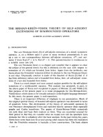
Now we will evaluate the y–eigenvalue for each of the poset tableaux for this L-block.
The only nontrivial node is node 4. Thus, the y–eigenvalue, e
y
(Λ), is the node-eigenvalue,
e
4
(Λ) = c(1, 2) + c(1, 3) −

2
2

.Theresultisgiveninfigure2.
Note that the y–eigenvalues of this labeling give exactly the same numbers as the eigen-
values of the Laplacian L
Y
. In the next section we will show that this is not coincidental.
the electronic journal of combinatorics 2 (1995), #R14 21

∅
r
r
r
r
r
e
y
(Λ) = 2
∅
r
r
r
r
r
e
y
(Λ) = −1
∅
r
r
r
r
r
e
y
(Λ) = −1
Figure 2: Example: the y-eigenvalues
5 Centerpiece Theorem for L
Y

Theorem 14 (L
Y
-Centerpiece) Let P be a linear poset with a minimum element,
ˆ
0.Let
X and Y be two (multi-)sets, subsets of P . For every labeling Λ of positive multiplicity,
each element in e
y
(Λ) is an eigenvalue of L
Y
with multiplicity

x-nodes v
m
v
(Λ).
Proof:
The proof of this theorem will be by induction on the sizes of the (multi)-sets X and
Y .Soletn = |X| = |Y | (counting multiplicities).
If n = 1 — there is nothing to prove as the Laplacian L
Y
has no pairs to switch, and
the only y-node is the maximal element for the diagram of the L-block. The Laplacian L
Y
istheone-by-onezeromatrixandtheeigenvalueofthisuniquepairiszero.
Suppose n = 2. There are several different possible combinations of relations between
sets X = {x
1
,x
2

} and Y = {y
1
,y
2
}.
• The most obvious one is x
1
<x
2
<y
1
<y
2
. In that case the Laplacian L
Y
=(y
1
,y
2
),
and the two possible elements are ζ
1
= z
x
1
,y
1
∧z
x
2

,y
2
, ζ
2
= z
x
1
,y
2
∧z
x
2
,y
1
. The Laplacian
L
Y
has the following matrix representation with respect to the basis ζ
1
,ζ
2
:
L
Y
=

01
10

The eigenvalues of L

Y
are +1 and −1. The eigenvalue of the poset tableau of type
(X,Y )
P
is given in figure 3. It also gives values +1 and −1, so the claim of the
theorem holds.
the electronic journal of combinatorics 2 (1995), #R14 22
∅
r
r
r
r
e
y
(Λ) = +1
∅
r
r
r
r
e
y
(Λ) = −1
Figure 3: poset tableaux



❅
❅
❅

∅
·
r
r
rr
e
y
(Λ) = 0



❅
❅
❅
∅
·
r
r
rr
e
y
(Λ) = 0
Figure 4: poset tableaux
• The second case is when
x
1
<x
2
<
y

1
y
2
In that case the Laplacian L
Y
does nothing (since y
1
and y
2
are not comparable),
thus the eigenvalues of L
Y
are 0. The dimension of the L-block spanned by (X, Y )
is two. The eigenvalues of the poset tableaux give the same values (figure 4), where
the ”·” in a box denotes which square was deleted in that step.
Thus in this case the theorem checks too.
• x
1
<y
1
<x
2
<y
2
or equivalently (for our purpose) x
1
<y
1
= x
2

<y
2
.
There is only one poset tableau spanned by these sets X and Y , namely the one
shown on the figure 5.
The y-eigenvalue for the poset tableau is zero in both cases.
The Laplacian L
Y
can not switch the y’s, since that would produce the element z
x
2
,y
1
which doesn’t exist. So the Laplacian L
Y
also acts as zero.
the electronic journal of combinatorics 2 (1995), #R14 23
∅
∅
r
r
r
r
e
y
(Λ) = 0
Figure 5: poset tableau
∅
r
r

r
e
y
(Λ) = 0
Figure 6: poset tableau
• x
1
<x
2
<y
1
= y
2
.
There is only one poset tableau spanned by these sets X and Y , namely the one
shown on the figure 6.
The y-eigenvalue is again zero (contents of the partition (2) minus the binomial
coefficient

2
2

). The Laplacian L
Y
doesn’t have two distinct y’s to switch, thus, it
is zero.
• x’s are the same.
x
1
= x

2
<
y
1
y
2
There is only one poset tableau spanned by these sets X and Y , namely the one
shown on the figure 7.
The y-eigenvalue is zero. The Laplacian L
Y
has no comparable y’s to switch - thus
L
Y
=0.
• x
1
= x
2
<y
1
<y
2
. There is only one poset tableau spanned by these sets X and Y ,
namely the one shown on the figure 8.
The y-eigenvalueisequalto1. TheLaplacianL
Y
can switch y
1
and y
2

but the result
would be the same element, since the x’s are indistinguishable. Thus the Laplacian
the electronic journal of combinatorics 2 (1995), #R14 24



❅
❅
❅
∅
r
rr
e
y
(Λ) = 0
Figure 7: poset tableau
∅
r
r
r
e
y
(Λ) = 1
Figure 8: poset tableau
L
Y
= Id, with the eigenvalue 1.
• In the trivial case when the x’s are not comparable the y’s are not comparable because
of linearity and the existence of a minimal element. So we have
x

1
<y
1
x
2
<y
2
.
The poset tableau again gives zero as the y-eigenvalue, and since the y’s are not
comparable, the Laplacian L
Y
is also zero.
So the theorem holds for the case n =2.
Now, we will treat the general case n>2.
• Label the y-nodes of the diagram of the L-block using the depth-first algorithm:
1. Start with a leftmost minimal y-element v.
2. If v is not the maximal unlabeled y-node go to the leftmost unlabeled cover of
v, and repeat this step. Otherwise label v with next available number from the
set {1, 2, , |Y |}.
From this labeling we see that, y
i
>y
j
⇒ i<j.
• Let P [X
1
,Y
1
],P[X
2

,Y
2
], ,P[X
c
,Y
c
] be the connected components of P[X, Y ]. In
that case the L-block V is the tensor product of the L-blocks of the P [X
i
,Y
i
]. The
the electronic journal of combinatorics 2 (1995), #R14 25
Laplacian L
Y
switches only comparable y’s, and two y’s from different connected
components are not comparable. Thus
L
Y
(v
1
⊗···⊗v
c
)=
c

i=1
v
1
⊗···⊗(L

Y
i
v
i
) ⊗···⊗v
c
.
So if v
1
, ,v
c
are eigenvectors of L
Y
with the eigenvalues e
1
, ,e
c
,thenv
1
⊗···⊗v
c
is an eigenvector with eigenvalue e
1
+ ···+ e
c
. Thus, by induction, we can label each
of the components of P [X, Y ] to get the eigenvalues of L
Y
on the total L-block V .
• Suppose that P [X,Y ] is connected. In that case, there must be a minimal element

in P [X, Y ], which must be an x-node.
Call the minimal element x
n
. Then define x
n−1
,x
n−2
, ,x
a
by:
1. x
a
>x
a+1
> ··· >x
n
,whereall> are covering relations.
2. Either
Case 1: There is more than one element covering x
a
.
Case 2: x
a
has unique cover in P [X, Y ] but it is a y-element.
Let B = {x
a
, ,x
n
},andletG =Sym(B).
Lemma 15 Let σ ∈ G,andletζ = z

x
i
1
,y
1
∧ z
x
i
2
,y
2
∧···∧z
x
i
n
,y
n
be non-zero. Then
ζ
σ
= z
σ(x
i
1
),y
1
∧ z
σ(x
i
2

),y
2
∧···∧z
σ(x
i
n
),y
n
is also non-zero.
Proof: It is sufficient to prove the lemma for the transposition (x
i
k
,x
i
l
) ∈ G.
ζ
(x
i
k
,x
i
l
)
= z
x
i
1
,y
1

∧···∧z
x
i
l
,y
l
∧···∧z
x
i
k
,y
k
∧···∧z
x
i
n
,y
n
.
Now, since (x
i
k
,x
i
l
) ∈ B, i.e., x
i
k
,x
i

l
are both less or equal to x
a
, which is below all
of the y’s–thelemmaisclear.
Lemma 16 This action of G commutes with L
Y
.
Proof: Let ζ = z
x
i
1
,y
1
∧ z
x
i
2
,y
2
∧···∧z
x
i
n
,y
n
be in our L-block, V ,lety
k
<
P

y
l
and let
σ ∈ G.Then
σ · (y
k
,y
l
) · ζ = z
σ(x
i
1
),y
1
∧···∧z
σ(x
i
k
),y
l
∧···∧z
σ(x
i
l
),y
k
∧···∧z
σ(x
i
n

),y
n
and
(y
k
,y
l
) · σ · ζ = z
σ(x
i
1
),y
1
∧···∧z
σ(x
i
k
),y
l
∧···∧z
σ(x
i
l
),y
k
∧···∧z
σ(x
i
n
),y

n
.