Báo cáo toán học: " Matrices connected with Brauer’s centralizer algebras" potx
Bạn đang xem bản rút gọn của tài liệu. Xem và tải ngay bản đầy đủ của tài liệu tại đây (383.11 KB, 39 trang )
Matrices connected with Brauer’s centralizer
algebras
∗
Mark D. McKerihan
†
Department of Mathematics
University of Michigan
Ann Arbor, MI 48109
Submitted: October 9, 1995; Accepted: October 31,1995
Abstract
In a 1989 paper [HW1], Hanlon and Wales showed that the algebra
structure of the Brauer Centralizer Algebra A
(x)
f
is completely determined
by the ranks of certain combinatorially defined square matrices Z
λ/µ
,
whose entries are polynomials in the parameter x. We consider a set of
matrices M
λ/µ
found by Jockusch that have a similar combinatorial de-
scription. These new matrices can be obtained from the original matrices
by extracting the terms that are of “highest degree” in a certain sense.
Furthermore, the M
λ/µ
have analogues M
λ/µ
that play the same role
that the Z
λ/µ
play in A
(x)
f
, for another algebra that arises naturally in
this context.
We find very simple formulas for the determinants of the matrices
M
λ/µ
and M
λ/µ
, which prove Jockusch’s original conjecture that det M
λ/µ
has only integer roots. We define a Jeu de Taquin algorithm for standard
matchings, and compare this algorithm to the usual Jeu de Taquin algo-
rithm defined by Sch¨utzenberger for standard tableaux. The formulas for
the determinants of M
λ/µ
and M
λ/µ
have elegant statements in terms of
this new Jeu de Taquin algorithm.
Contents
1Introduction 2
1.1 Acknowledgments 8
∗
Subject Class 05E15, 05E10
†
This research was supported in part by a Department of Education graduate fellowship
at the University of Michigan
1
the electronic journal of combinatorics 2 (1995),#R23 2
2 Determinants of M and M 8
2.1 Columnpermutationsofstandardmatchings 8
2.2 Product formulas for M and M 12
2.3 Eigenvalues of T
k
(x)andT
k
(y
1
, ,y
n
) 13
2.4 The column span of P 14
2.5 Computation of det M and det M 19
3 Jeu de Taquin for standard matchings 23
3.1 Definitionofthealgorithm 23
3.2 JeudeTaquinpreservesstandardness 25
3.3 DualKnuthequivalencewithJdTfortableaux 31
3.4 ThenormalshapeobtainedviaJdT 35
3.5 Analternatestatementofthemaintheorem 38
1Introduction
Brauer’s Centralizer Algebras were introduced by Richard Brauer [Brr] in 1937
for the purpose of studying the centralizer algebras of orthogonal and sym-
plectic groups on the tensor powers of their defining representations. An in-
teresting problem that has been open for many years now is to determine the
algebra structure of the Brauer centralizer algebras A
(x)
f
. Some results about the
semisimplicity of these algebras were found by Brauer, Brown and Weyl, and
have been known for quite a long time (see [Brr],[Brn],[Wl]). More recently,
Hanlon and Wales [HW1] have been able to reduce the question of the structure
of A
(x)
f
to finding the ranks of certain matrices Z
λ/µ
(x). Finding these ranks
has proved very difficult in general. They have been found in several special
cases, and there are many conjectures about these matrices which are supported
by large amounts of computational evidence. One conjecture arising out of this
work was that A
(x)
f
is semisimple unless x is a rational integer. Wenzl [Wz] has
used a different approach (involving “the tower construction” due to Vaughn
Jones [Jo]) to prove this important result. In our work we take the point of
view taken by Hanlon and Wales in [HW1]-[HW4], and we pay particular atten-
tion to the case where x is a rational integer.
We consider subsets of
+
×
+
, which we will think of as the set of positions
in an infinite matrix, whose rows are numbered from top to bottom, and whose
columns are numbered from left to right. Thus, the element (i, j) will be thought
of as the position in the ith row, and jth column of the matrix. These positions
will be called boxes.
Definition 1.1. Define the partial order <
s
, “the standard order” on
+
×
+
,
by x ≤
s
y if x appears weakly North and weakly West of y.
Definition 1.2. Define the total order <
h
, “the Hebrew order” on
+
×
+
,
by x<
h
y if y is either strictly South of x,orify is in the same row as x and
strictly West of x in that row.
the electronic journal of combinatorics 2 (1995),#R23 3
Definition 1.3. A finite subset D ⊂
+
×
+
will be called a diagram.A
matching of the diagram D is a fixed point free involution : D → D.A
matching δ of the diagram D is called standard if for every x, y ∈ D, x<
s
y
implies that δ(x) <
h
δ(y).
We will usually use to denote an arbitrary matching, while δ will be reserved
for standard matchings.
It will sometimes be convenient to think of matchings in a slightly different
way, namely as 1-factors. A 1-factor is a graph such that every vertex is incident
with exactly one edge. If isamatchingofD, then we can think of as a 1-
factor by putting an edge between x and (x) for all x ∈ D. Note that if there
isamatchingofshapeD, then D mustcontainanevennumberofboxes.
Example 1.1. There are three matchings of shape (4,2)/(2). They are repre-
sented below as the 1-factors δ, δ
and . The matchings δ and δ
are both
standard, while is not standard.
δ
ε
δ
’
==
=
Remark 1.1. An immediate consecuence of the definition for a standard match-
ing is that one can never have an edge between boxes x and y if both x<
s
y and
x<
h
y. This means that there can be no NW-SE edges in a standard matching,
nor N-S (or vertical) edges. There can be E-W (horizontal) edges however.
Let F
D
be the set of matchings of D,andletV
D
be the real vector space
with basis F
D
.LetA
D
be the set of standard matchings of D.
If λ/µ isaskewshapethenlet[λ/µ] ⊂
+
×
+
be the set of boxes (i, j)
such that µ
i
<j≤ λ
i
.IfD =[λ/µ] for some skew shape λ/µ, then we
will sometimes drop the brackets, especially in subscripts. For example, by
convention F
λ/µ
= F
[λ/µ]
.
Suppose that λ/µ is a skew shape. Let S
λ/µ
denote the symmetric group on
the set [λ/µ]. There is an S
λ/µ
action on F
λ/µ
given by
(π)(x)=π((π
−1
x)) (1.1)
where π ∈ S
λ/µ
. In terms of 1-factors, this is equivalent to saying that x and y
are adjacent in if and only if π(x)andπ(y)areadjacentinπ.
Let C
λ/µ
(resp. R
λ/µ
), the column stabilizer (resp. row stabilizer) of [λ/µ],
be the subgroup of S
λ/µ
, consisting of permutations π, such that π(x)isinthe
same column (resp. row) as x, for all x ∈ [λ/µ].
If
1
and
2
are matchings of shape [λ/µ], we obtain a new graph on the
vertex set [λ/µ] by simply superimposing the two matchings. We denote this
new graph by
1
∪
2
.Wedefineγ(
1
,
2
) to be the number of cycles in
1
∪
2
(which is the same as the number of connected components in
1
∪
2
).
Example 1.2. Below are two matchings of shape (5,4,2)/(2,1),
1
and
2
.Here
γ(
1
,
2
)=2.
the electronic journal of combinatorics 2 (1995),#R23 4
=ε
1
εε
12
=
ε
2
=
We define the A
λ/µ
× A
λ/µ
matrix M = M
λ/µ
(x) as follows:
M
ij
= M
δ
i
,δ
j
=
σ∈C
λ/µ
τ ∈R
λ/µ
sgn(σ)x
γ(στδ
i
,δ
j
)
(1.2)
where A
λ/µ
= {δ
1
, δ
s
}.
We have defined a matching of shape λ/µ to be a fixed point free involution
of [λ/µ], or equivalently a 1-factor on [λ/µ]. If |µ| = m,and|λ/µ| =2k, then
we can also think of a matching of shape λ/µ as a labelled (m, k) partial 1-
factor on the set [λ]. A labeled (m, k) partial 1-factor is a graph on f = m +2k
points, where 2k points are incident with exactly one edge, and m points (called
free points) are incident with no edges. These free points are labelled with the
numbers 1, 2, ,m. For a matching of shape λ/µ, the free points are the boxes
in [µ],andwelabeltheminorderfromlefttorightineachrow,fromthetop
row to the bottom row.
Let P
λ,m
be the set of labelled (m, k) partial 1-factors on [λ]. There is an
S
λ
action on P
λ,m
given by saying that x and y are adjacent in ,ifandonly
if π(x)andπ(y)areadjacentinπ,andifx is a free point in with label i,
then π(x) is a free point in π with label i. Note that F
λ/µ
⊆ P
λ,m
and that the
S
λ/µ
action we defined on F
λ/µ
is equivalent to the restriction of the S
λ
action
on F
λ/µ
to those permutations in S
λ
that fix [µ] pointwise. As before, we define
R
λ
(resp. C
λ
) to be the subgroup of S
λ
that stabilizes the rows (resp. columns)
of λ.
Suppose that
1
,
2
are labelled (m, k) partial 1-factors in P
λ,m
. Then
1
∪
2
is a graph on the vertex set [λ] consisting of exactly m paths (an isolated point
is considered a path of length zero), and some number γ(
1
,
2
) of cycles, each of
which has even length. Each of the m paths is a path from one labelled point to
another. Let ζ(
1
,
2
) equal 1 if each path has the same label at both endpoints,
and 0 otherwise. We can now define Z = Z
λ/µ
(x) as follows.
Z
ij
= Z
δ
i
,δ
j
=
σ∈C
λ
τ ∈R
λ
sgn(σ)ζ(στδ
1
,δ
2
)x
γ(στδ
i
,δ
j
)
(1.3)
The terms that appear in M are a subset of those that appear in Z because if
σ ∈ C
λ/µ
then σ fixes [µ] pointwise, and the same is true for all τ ∈ R
λ/µ
.Thus,
the electronic journal of combinatorics 2 (1995),#R23 5
στ fixes [µ] pointwise, and it follows that ζ(στδ
i
,δ
j
) = 1 for all i, j.Onecan
think of M as the component of Z that leaves [µ] fixed. In this paper, we are able
to find the determinant of M precisely. In order to find the determinant of Z,
one might try to get an intermediate result which would involve matrices which
only allowed the boxes in [µ] to move in certain restricted ways. If one could get
results about such matrices, and then find a way to remove the restrictions, one
might finally arrive at the determinant of Z. This would be a powerful tool for
finding the rank of Z, which is equivalent to determining the algebra structure
of A
(x)
f
completely.
If x = n ∈
+
, one can generalize the definition of the matrix Z by intro-
ducing power sum symmetric functions to keep track of the lengths of cycles.
Recall that for i ≥ 0, the ith power sum on y
1
, ,y
n
is given by
p
i
(y
1
, ,y
n
)=
n
j=1
y
i
j
. (1.4)
Note that p
i
(1, ,1) = n for all i. For any partition ν =(ν
1
,ν
2
, ,ν
l
), we
define p
ν
=
p
ν
i
.If
1
and
2
are labelled (m, k) partial 1-factors in P
λ,m
, then
define Γ(
1
,
2
) to be the partition having one part for each cycle in
1
∪
2
.If
a cycle in
1
∪
2
has length 2r, then its corresponding part in Γ(
1
,
2
)isr.
Example 1.3. Below are two (3, 4) partial 1-factors,
1
and
2
.Inthisexample
γ(
1
,
2
)=2,Γ(
1
,
2
)=(2, 1) and ζ(
1
,
2
)=1.
=ε
1
εε
12
=
ε
2
=
12
3
2
31
22
33
1
1
Define Z = Z
λ/µ
(y
1
, ,y
n
)by
Z
ij
= Z
δ
i
,δ
j
=
σ∈C
λ
τ∈R
λ
sgn(σ)ζ(στδ
1
,δ
2
)p
Γ(στδ
i
,δ
j
)
. (1.5)
It is clear that Z
λ/µ
(1, ,1) = Z
λ/µ
(n).
In [HW1], Hanlon and Wales show that if µ = ∅ and λ consists entirely
of even parts (such a partition is called even), then Z
λ/µ
(y
1
, ,y
n
) is a one
by one matrix whose only entry is a scalar multiple of the zonal polynomial
z
ν
(y
1
, ,y
n
) where λ =2ν (i.e. λ
i
=2ν
i
for all i). Zonal polynomials
the electronic journal of combinatorics 2 (1995),#R23 6
were introduced by A.T. James (see [Ja1]-[Ja3]) in connection with his work
on multidimensional generalizations of the chi-squared distribution. Here we
will just say that z
ν
is a homogeneous symmetric function of degree |ν|,and
z
ν
(1, ,1) = h
λ
(n), where h
λ
(x) is the single entry of the matrix Z
λ/∅
(x). A
formula for h
λ
(x) is given in [HW1] which we state as Theorem 2.6.
If |λ/µ| =2k, then in terms of the monomials y
i
1
1
···y
i
n
n
, the entries of
the matrix Z have degree at most k. To see this, observe that the degree of
p
Γ(στδ
i
,δ
j
)
is equal to |Γ(στδ
i
,δ
j
)|, and that |Γ(στδ
i
,δ
j
)|≤k because there are
2k edges in στδ
i
∪ δ
j
.Ifall2k edges are contained in cycles then the term will
have degree k, but if any edges are contained in paths, then the degree will be
smaller than k.
Define M = M
λ/µ
(y
1
, ,y
n
) to be the matrix obtained from Z by extract-
ing the terms of degree k.Thus,M will be a matrix consisting entirely of zeroes
and terms of degree k. As we noted above, in order for a term in Z to have
degree k,everyedgeinστδ
i
∪ δ
j
must be contained in a cycle, or equivalently
every path must be an isolated point (and this point must have the same label
in στδ
i
and δ
j
). It is not hard to see that this happens if and only if τ and σ
are both in S
λ/µ
,i.e. bothfix|µ| pointwise. Hence
M
ij
= M
δ
i
,δ
j
=
σ∈C
λ/µ
τ∈R
λ/µ
sgn(σ)p
Γ(στδ
i
,δ
j
)
. (1.6)
It follows that M
λ/µ
(1, ,1) = M
λ/µ
(n). In this sense, the matrix M
can be considered the “highest degree” part of the matrix Z, where we are
computing the “degree” of the terms using the homogeneous degree of the cor-
responding terms in the matrix Z. For example, the terms p
2
p
1
and p
3
1
have
the same homogeneous degree three. But when we specialize p
2
= p
1
= n, the
corresponding terms are n
2
and n
3
respectively. In the sense described above
however, both terms have “degree” equal to three. Also, there is more than
one way to obtain n
i
for any i>1. This means that one generally cannot
reconstruct M by substitution in M(n).
The matrix M has an interesting algebraic interpretation which we briefly
describe here. To do this we give a short description of the algebra A
(x)
f
and
the closely related algebra A
Λ
f
. See [HW1] for a more complete description.
Both algebras have the same basis, namely the set of 1-factors on 2f points.
To define the product of two such 1-factors δ
1
and δ
2
,weconstructagraph
B(δ
1
,δ
2
). We can think of this graph as a 1-factor β(δ
1
,δ
2
)togetherwithsome
number γ(δ
1
,δ
2
)ofcyclesofevenlengths2l
1
, 2l
2
, ,2l
γ(δ
1
,δ
2
)
. The product in
A
(x)
f
is given by
δ
1
∗ δ
2
= x
γ(δ
1
,δ
2
)
β(δ
1
,δ
2
).
In A
Λ
f
, the product is
δ
1
· δ
2
=
γ(δ
1
,δ
2
)
j=1
p
l
j
(y
1
, ,y
n
)
β(δ
1
,δ
2
)
the electronic journal of combinatorics 2 (1995),#R23 7
where p
i
(y
1
, ,y
n
) is the ith power sum. Since p
i
(1, ,1) = n for all i, the
specialization of A
Λ
f
to y
1
= ··· = y
n
= 1 is isomorphic to A
(n)
f
.
In A
Λ
f
there is an important tower of ideals A
Λ
f
= A
Λ
f
(0) ⊃ A
Λ
f
(1) ⊃ A
Λ
f
(2) ⊃
···.LetD
Λ
f
(k)=A
Λ
f
(k)/A
Λ
f
(k + 1). In [HW1], Hanlon and Wales express the
multiplication in D
Λ
f
(k) in terms of a matrix Z
m,k
= Z
m,k
(y
1
, ,y
n
) where
f = m +2k. Furthermore, they show that the algebra structure of D
Λ
f
(k)for
particular values of y
1
, ,y
n
is completely determined by the rank of Z
m,k
.
Their work implies that det(Z
m,k
) = 0 for the values y
1
, ,y
n
if and only if
D
Λ
f
(k) is semisimple for those values.
A typical element of D
Λ
f
(k) is a sum of terms of the form fδ where f is
a homogeneous symmetric function and δ is a certain type of 1-factor. Let
gr(fδ)=deg(f)+k. The multiplication in D
Λ
f
(k) respects this grading in the
sense that gr(f
1
δ
1
· f
2
δ
2
) ≤ gr(f
1
δ
1
) + gr(f
2
δ
2
). Let
˜
D
Λ
f
(k)betheassociated
graded algebra. One can construct matrices M
m,k
= M
m,k
(y
1
, ,y
n
)that
play the same role in
˜
D
Λ
f
(k) that the Z
m,k
play in D
Λ
f
(k). It turns out that
M
m,k
is the matrix obtained from Z
m,k
by extracting highest degree terms.
Using the representation theory of the symmetric group, one can show that
the matrix M
m,k
is similar to a direct sum of matrices M
λ/µ
where λ and µ
are partitions of f and m respectively. These matrices M
λ/µ
are precisely the
matrices M defined above. The main result of this paper is a formula for the
determinant of M, which can be interpreted as a discriminant for the algebra
˜
D
Λ
f
(k) in the same way that det Z is a discriminant for D
Λ
f
(k).
This paper is split into two main sections. In section 2, we prove several basic
facts about standard matchings which are needed to compute the determinant
of M. In particular, we find an ordering on matchings (defined in 2.4) such
that if δ is a standard matching, then any column permutation of δ yields a
matching which is weakly greater than δ in this order (see Theorem 2.5). In
Theorem 2.11 we show that the standard matchings of shape λ/µ index a basis
for an important vector space associated to λ/µ. This part of the paper is very
similar in flavor to standard constructions of the irreducible representations of
the symmetric group. Using these two theorems, we are able to give an explict
product formula for the determinant of M in Theorem 2.14. This formula has
the following form:
det M = C
2ν|λ/µ|
h
2ν
(x)
c
λ
µ 2ν
where C is some nonzero real number, and c
λ
µν
is a Littlewood-Richardson co-
efficient. The same argument also shows that for x = n ∈
+
,
det M = C
2ν|λ/µ|
z
ν
(y
1
, ,y
n
)
c
λ
µ 2ν
where the constant C is the same as the one above.
In section 3, we introduce a Jeu de Taquin algorithm for standard match-
ings. Much of this section is devoted to a comparison of this algorithm with
the electronic journal of combinatorics 2 (1995),#R23 8
the well known Jeu de Taquin algorithm for standard tableaux invented by
Sch¨utzenberger. This makes sense because there is a natural way to think
about any matching as a tableau such that a matching is standard if and only
if it is standard as a tableau. In Theorem 3.3 we show that if Jeu de Taquin
for matchings is applied to a standard matching of a skew shape with one box
removed, then the output is another standard matching. Theorem 3.5 gives a
description of how the two Jeu de Taquin algorithms compare in terms of the
dual Knuth equivalence for permutations. Theorem 3.5 is used to show in The-
orem 3.10 that if Jeu de Taquin is used to bring a standard matching of a skew
shape to a standard matching of a normal shape (the shape of a partition), then
both algorithms arrive at the same normal shape, and as a consequence of this,
the standard matching of normal shape obtained from any standard matching
is independent of the sequence of Jeu de Taquin moves chosen. Finally, using
Theorem 3.12, a result of Dennis White [Wh] we find that the number of times
the normal shape ν appears as the shape obtained from a standard matching
of shape λ/µ using Jeu de Taquin is the Littlewood-Richardson coefficient c
λ
µν
(Theorem 3.14). Using this theorem we obtain elegant restatements of the main
results from section 2 (Theorems 2.14 and 2.16) in terms of the Jeu de Taquin
algorithm for standard matchings.
1.1 Acknowledgments
The author would like to thank William Jockusch for suggesting the problem
discussed in this paper, and Phil Hanlon for valuable discussions leading to the
results described here.
2 Determinants of
M
and
M
2.1 Column permutations of standard matchings
Definition 2.1. Suppose is a matching of shape λ/µ. Define T () to be the
filling of [λ/µ] that puts i in box x if (x)isinrowi. Define
T () to be the
filling obtained by rearranging the elements in each row of T()inincreasing
orderfromlefttoright.
Example 2.1. Here are T ()and
T () for the matching shown below.
εT( )
233
1225
14
2
33
41
=
εT( )
1
11
22
2
3
3
5
3
44
23
=ε =
Lemma 2.1. If δ is a standard matching then T (δ) is a semistandard tableau.
the electronic journal of combinatorics 2 (1995),#R23 9
Proof. Suppose x ∈ [λ/µ]. If y ∈ [λ/µ] is immediately below or to the right of x
then x<
s
y.Henceδ(x) <
h
δ(y), and it follows that δ(y) must be in the same
row as δ(x)orbelow.
If y ∈ [λ/µ] is immediately below x, then δ(y) cannot be in the same row
as δ(x) because if that were the case, then δ(y) would have to be to the left of
δ(x), i.e. δ(y) <
s
δ(x). But this implies that y<
h
x, a contradiction.
Thus, T (δ) increases weakly in its rows, and strictly in its columns.
Remark 2.1. Lemma 2.1 implies that if δ is a standard matching, then T (δ)=
T (δ).
Also, it is not hard to see that δ → T(δ) is a bijection between standard
matchings of shape λ/µ and semistandard tableaux of shape λ/µ satisfying
1. Row i hasanevennumberofi’s, and
2. Row i has kj’s if and only if row j has ki’s.
For the notation described below and the following two lemmas, let δ be
some fixed standard matching of shape λ/µ.
Notation . Let R
i
denote the ith row of [λ/µ]. If x ∈ [λ/µ] then let row(x)
denote the row number in which x appears. For all i ∈ let C
i
denote the
subset of [λ/µ] defined as follows:
If i ≥ 0 then C
i
is the union of the columns of [λ/µ] that have an i +1in
the first row of
T (δ)=T (δ).
If i<0 then C
i
is the union of the columns of [λ/µ] whose top box is in row
|i| +1=1− i.
the electronic journal of combinatorics 2 (1995),#R23 10
Example 2.2. Below is T (δ) for a standard matching for which the sets R
i
and
C
i
are shown.
2
1
4
33
4
CC
R
1
R
R
R
R
2
3
4
5
-1-4
2
31
22
1
5
3
CC
14
δ = T( )=δ
Remark 2.2. Note that R
i
∩ C
j
= ∅ unless j ≥ 1 − i.
Lemma 2.2. Suppose x ∈ C
i
,andδ(x) ∈ C
j
.Then
a. row(δ(x)) ≥ row(x)+i,androw(x) ≥ row(δ(x)) + j,
b. i + j ≤ 0,and
c. If i = −j,thenrow(x)=row(δ(x)) + i,i.e.x is exactly i rows below
δ(x).
Proof. Suppose x ∈ R
k
,andδ(x) ∈ R
l
.InT(δ), position x has an l in it.
Lemma 2.1 implies that l ≥ k + i, which is precisely the first statement in a.
The second statement in a follows from the first by noting that δ(δ(x)) = x.
Both b and c are immediate consequences of a.
Lemma 2.3. Suppose i ≥ 0,andx ∈ C
i
satisfies row(δ(x)) = row(x)+i.
Suppose also that there are k columns in C
i
to the right of x. Then there are
no more than k columns in C
−i
to the left of δ(x).
Proof. Let z be a box in R
row(δ(x))
∩ C
−i
that lies to the left of δ(x). We have
z<
s
δ(x), so δ(z) <
h
x.Thus,δ(z)liesinR
row(x)
or above. But Lemma 2.2 a
implies that
row(δ(z)) ≥ row(z) − i =row(x)(2.1)
i.e. δ(z)liesinR
row(x)
or below. Furthermore, Lemma 2.2 b says that δ(z)lies
in C
i
or to its left. Therefore, δ(z)liesinR
row(x)
∩ C
i
andtotherightofx.
The number of such boxes z is obviously bounded by k.
One useful consequence of these two lemmas is the following Corollary.
Corollary 2.4. Suppose λ 2k.Then,ifλ is even, there is exactly one stan-
dard matching of shape λ.Ifλ is not even, then there are no standard matchings
of shape λ.
the electronic journal of combinatorics 2 (1995),#R23 11
Proof. Suppose that δ is a standard matching of shape λ. Observe that because
λ is normal, C
i
= ∅ for all i<0. But now, Lemma 2.2 b implies that C
i
= ∅ for
all i>0 as well. Thus [λ]=C
0
.
Now, by Lemma 2.2 c, all edges of δ must be horizontal, which implies
immediately that λ is even. Furthermore, for a single row of an even number of
boxes, it is not hard to see that there is exactly one matching that is standard,
namely the one that connects the ith box from the left to the ith box from the
right of the row. Putting all of these rows together, we see that the resulting
matching is indeed standard.
Definition 2.2. Define the total order ≺ on tableaux of shape λ/µ with weakly
increasing rows as follows:
Wri te S ≺ T , if the word w
S
obtained by reading the rows of S from left
to right, from the top row to the bottom row, lexicographically precedes the
corresponding word w
T
, obtained by reading T in the same order.
Remark 2.3. Note that ≺ induces a total order on standard matchings (but
not all matchings) of shape λ/µ,viaδ
1
≺ δ
2
if and only if T (δ
1
) ≺ T(δ
2
). This
follows from Remark 2.1, which implies that a standard matching δ is completely
determined by
T (δ). Note that this is not true of matchings in general. In other
words, there could be several matchings with the same associated tableau, but
there can be at most one standard matching associated to any tableau.
Theorem 2.5. Suppose σ ∈ C
λ/µ
,andsupposeδ is a standard matching of
shape λ/µ.Then
T (σδ) T(δ),andT(σδ)=T (δ) if and only if σδ = δ.
Proof. We induct on |[λ/µ]|.If|[λ/µ]| = 2, the statement of the theorem is
trivially true since there is only one matching of shape λ/µ in that case.
If |[λ/µ]| > 2, then let k be the smallest nonnegative integer such that
C
k
= ∅,i.e. k + 1 is the entry of T(δ) in the leftmost box of the first row. Let
H be the subgroup of the column stabilizer of [λ/µ] consisting of permutations
τ such that (τδ)(x)=δ(x) for all x ∈ R
1
∩ C
k
.
Let A = R
1
∩ C
k
,andletα (resp. β) be the word obtained by reading the
entries corresponding to the positions of A in
T (δ)(resp. T(σδ)) from left to
right. Note that α is a word consisting entirely of k +1’s.
First, we will show that β cannot precede α in the lexicographic order. Then,
we will show that if β = α,thenσ ∈ H. Once we have shown these two things,
we will be able to finish the proof of the theorem by induction.
To show that β does not precede α lexicographically, we show that β cannot
contain any letters smaller than k +1. If β contained l<k+ 1, then for some
x ∈ R
1
,(σδ)(x) ∈ R
l
. Suppose x ∈ C
i
. Note that i ≥ k,and(σδ)(x) ∈ C
j
for some j ≥ 1 − l>−k. (Recall that R
l
∩ C
j
= ∅ unless j ≥ 1 − l). Since
σ stabilizes the columns of [λ/µ], this implies that there exists some z ∈ C
i
such that δ(z) ∈ C
j
.Buti + j>k− k = 0, which contradicts Lemma 2.2
b. We conclude that β cannot precede α lexicographically. Observe that this
same argument shows that if x ∈ R
1
and (σδ)(x) ∈ R
k+1
, then x ∈ C
k
,and
(σδ)(x) ∈ C
−k
.
the electronic journal of combinatorics 2 (1995),#R23 12
Suppose now that β = α, and suppose that σ/∈ H. Write the elements of A
as x
1
,x
2
, ,x
a
in order from right to left, and let x
i
be the rightmost box in
A such that y =(σδ)(x
i
) = δ(x
i
). In R
k+1
,lety
1
,y
2
, ,y
a
be the first a boxes
from left to right. Note that for all j ∈{1, ,a}, δ(x
j
)=y
j
. Furthermore, for
each j ∈{1, ,a}, δ(y
j
)=x
j
∈ R
1
, and hence T (δ) has a 1 in position y
j
for
all such j. This implies that each such y
j
must be at the top of its column, and
hence in C
−k
.
Since β = α, y ∈ R
k+1
.Also,y = y
j
for any j ≤ i.Thusy is farther right in
R
k+1
than y
i
.Sinceσ stabilizes the columns of [λ/µ], this implies that there is
some z ∈ C
k
in the same column as x
i
, such that δ(z) is in the same column as
y. Now, by the comments above, δ(z)mustbeinC
−k
or to its right. Lemma
2.2 b implies that δ(z)mustbeinC
−k
or to its left. Thus δ(z) ∈ C
−k
, and now
Lemma 2.2 c implies that δ(z)isexactlyk rows below z. By Lemma 2.3, δ(z)
must be in the same column as y
i
, or to its left. But this contradicts the fact
that y lies to the right of y
i
and δ(z) is in the same column as y.Itfollowsthat
σ ∈ H as desired.
We have shown that
σ/∈ H =⇒
T (σδ) T(δ). (2.2)
If σ ∈ H then let µ
∗
be the partition such that [µ
∗
]=[µ] ∪ A ∪ δ(A). Let δ
∗
be
the standard matching of shape λ/µ
∗
that is δ restricted to [λ/µ
∗
]. Let σ
∗
∈ H
be a column permutation of [λ/µ] such that σ
∗
fixes A ∪ δ(A) pointwise, and
σ
∗
δ = σδ. Itisclearthatsuchaσ
∗
exists because of the definition of H.We
can think of σ
∗
as a column permutation of [λ/µ
∗
].
By induction, we have
T (σ
∗
δ
∗
) T (δ
∗
)(2.3)
and
T (σ
∗
δ
∗
)=T (δ
∗
) ⇐⇒ σ
∗
δ
∗
= δ
∗
. (2.4)
Now,
T (σδ)=T(σ
∗
δ) has the same letters as T (δ) in the positions in A ∪ δ(A),
so it is clear from (2.3) that T (σδ) T(δ). Moreover, (2.4) implies that T (σδ)=
T (δ) if and only if σδ = δ.
2.2 Product formulas for M and
M
For the remainder of this paper, we assume that |λ/µ| =2k. Itwillbeconvenient
to think of the matrices M and M as products of three matrices,
M = P
t
T
k
(x)J
M = P
t
T
k
(y
1
, ,y
n
)J.
(2.5)
Here, P is the F
λ/µ
× A
λ/µ
matrix with (, δ) entry equal to the coefficient
of in e(δ) ∈ V
λ/µ
, where e ∈ [S
λ/µ
] is given by
e =
σ∈C
λ/µ
τ ∈R
λ/µ
sgn(σ)στ. (2.6)
the electronic journal of combinatorics 2 (1995),#R23 13
In other words, P is the matrix whose ith column is the expansion of e(δ
i
)in
terms of the basis F
λ/µ
, where δ
i
is the ith standard matching of shape λ/µ.
The matrix T
k
(x) is the F
λ/µ
× F
λ/µ
matrix with (
1
,
2
)entrygivenby
T
k
(x)
1
,
2
= x
γ(
1
,
2
)
. (2.7)
We define T
k
(y
1
, ,y
n
)by
T
k
(y
1
, ,y
n
)
1
,
2
= p
Γ(
1
,
2
)
. (2.8)
Note that T
k
(x)andT
k
(y
1
, ,y
n
) are symmetric matrices.
The F
λ/µ
× A
λ/µ
matrix J is defined as follows:
J
,δ
=
1 = δ,
0 = δ.
(2.9)
We want to show that the (δ
i
,δ
j
)entryofP
t
T
k
(x)J is equal to the (δ
i
,δ
j
)
entry of M.IfY is any matrix, then let Y
denote the column of Y indexed by
.Wehave
(P
t
T
k
(x)J)
δ
i
,δ
j
= P
t
δ
i
T
k
(x)J
δ
j
= P
t
δ
i
T
k
(x)
δ
j
=
σ∈C
λ/µ
τ ∈R
λ/µ
sgn(σ)T
k
(x)
στδ
i
,δ
j
=
σ∈C
λ/µ
τ ∈R
λ/µ
sgn(σ)x
γ(στδ
i
,δ
j
)
= M
δ
i
,δ
j
.
(2.10)
Exactly the same argument shows that M = P
t
T
k
(y
1
, ,y
n
)J as well.
2.3 Eigenvalues of T
k
(x) and
T
k
(y
1
, ,y
n
)
Using the product formulas (2.5) for M and M, we can find product formulas for
det M and det M. We can do this because the matrices T
k
(x)andT
k
(y
1
, ,y
n
)
are known to have certain nice properties. What follows is a brief discussion of
these properties. For a more detailed discussion, see [HW1].
Recall that there is an S
λ/µ
action on F
λ/µ
given by
(σ)(x)=σ((σ
−1
x)). (2.11)
This action can be linearly extended to V
λ/µ
, which defines a representation
ρ : S
λ/µ
→ End(V
λ/µ
) as follows:
(ρ(σ))()=σ. (2.12)
The key fact about T
k
(x)andT
k
(y
1
, ,y
n
)thatweneedisthatbothcom-
mute with the action of S
λ/µ
. In other words, T
k
(x)andT
k
(y
1
, ,y
n
)can
the electronic journal of combinatorics 2 (1995),#R23 14
be regarded as endomorphisms of V
λ/µ
satisfying the following equations for all
σ ∈ S
λ/µ
:
ρ(σ)T
k
(x)=T
k
(x)ρ(σ)
ρ(σ)T
k
(y
1
, ,y
n
)=T
k
(y
1
, ,y
n
)ρ(σ)
(2.13)
This is an easy consequence of the following easy to prove identities (see [HW1]).
γ(σ
1
,σ
2
)=γ(
1
,
2
)
Γ(σ
1
,σ
2
)=Γ(
1
,
2
)
(2.14)
Furthermore, the S
λ/µ
action on F
λ/µ
is equivalent to the action on the
conjugacy class of fixed point free involutions of S
λ/µ
. It follows from ([M]
Ex.5, p.45) that
V
λ/µ
=
2ν
V
2ν
(2.15)
where the sum runs over all even partitions 2ν 2k. Here, V
2ν
denotes a
submodule of V
λ/µ
, isomorphic to the irreducible S
λ/µ
module indexed by 2ν.
In this notation, V
(2k)
is isomorphic to the trivial representation, while V
(1
2k
)
is
isomorphic to the sign representation.
Since V
λ/µ
decomposes into a direct sum of irreducibles V
2ν
, each of which
has multiplicity 1, it follows from Schur’s Lemma that T
k
(x) restricted to V
2ν
is a scalar operator denoted h
2ν
(x)I. Similarly, T
k
(y
1
, ,y
n
) restricted to V
2ν
is a scalar operator. Hanlon and Wales [HW1] compute both of these scalars.
Theorem 2.6. [HW1] Let 2ν 2k.Then
h
2ν
(x)=
(i,2j)∈[2ν]
(x +2j − i − 1).
Theorem 2.7. [HW1] Let 2ν 2k.ThenT
k
(y
1
, ,y
n
) restricted to V
2ν
is
the scalar operator z
ν
(y
1
, ,y
n
)I,wherez
ν
(y
1
, ,y
n
) is the zonal polynomial
indexed by ν.
2.4 The column span of P
In order to analyze M and M,wewillconsiderhowT
k
(x)andT
k
(y
1
, ,y
n
)
act on the column span of P . It turns out that this span is the same as the
space e(V
λ/µ
)=e(): ∈ F
λ/µ
, where e is defined in equation (2.6). We will
show, in fact, that the columns of P form a basis for this space.
Definition 2.3. We say that a matching of shape λ/µ is row (column) in-
creasing if every pair x<
s
y ∈ [λ/µ], that lie in the same row (column), satisfies
(x) <
h
(y).
Remark 2.4. By Lemma 3.1 A matching δ of shape λ/µ is standard if and only
if it is both row and column increasing.
the electronic journal of combinatorics 2 (1995),#R23 15
Lemma 2.8. For any matching ∈ F
λ/µ
, there exists a row permutation τ ∈
R
λ/µ
, such that τ is row increasing.
Proof. For this proof we use the description of a matching as a 1-factor. For
every i, we can choose a permutation π
(i)
which permutes row i as follows. All
the boxes in row i that are attached to row 1 are moved to the far left of row i.
The boxes that are attached to row 2 are moved to the right of those attached
to row 1 but to the left of every other box, and so on. So in π
(i)
,ifx is to the
left of y in row i, then
row(π
(i)
(x)) ≤ row(π
(i)
(y)). (2.16)
If j = i, then π
(i)
has no effect on the row to which any box in row j is attached.
Hence, if we let
π = π
(1)
π
(2)
, (2.17)
then π is a matching such that if x<
s
y are in the same row then
row(π(x)) ≤ row(π(y)). (2.18)
Let D
ij
be the set of boxes in row i that are adjacent to a box in row j in
π. Note that (D
ij
)=D
ji
. Equation 2.18 implies that D
ij
and D
ji
are sets of
consecutive boxes in their respective rows. We can assume that i ≤ j here, and
choose a permutation σ
(ij)
,ofD
ij
such that the kth box from the left of D
ij
is
attached to the kth box from the right of D
ji
in σ
(ij)
π. It is clear that σ
(ij)
π
restricted to D
ij
∪ D
ji
is row increasing.
Furthermore, σ
(ij)
has no effect on [λ/µ] \ (D
ij
∪ D
ji
), so if we let
σ =
i≤j
σ
(ij)
, (2.19)
then σπ is row increasing everywhere. Therefore, τ = σπ is the desired permu-
tation.
Now, if τ ∈ R
λ/µ
, it is clear from the definition of e in (2.6) that e(τ)=e().
This fact, together with Lemma 2.8 implies that we can reduce our spanning
set for e(V
λ/µ
)asfollows
e(V
λ/µ
)=e(): ∈ F
λ/µ
, row increasing (2.20)
Suppose that the matching of shape λ/µ is row increasing, but not column
increasing. Then there is a box x lying immediately above a box y such that
(x) >
h
(y). Let A be the set of boxes in [λ/µ] that are in the same row as y,
andatleastasfarWestasy.LetB be the set of boxes in [λ/µ] that are in the
same row as x, and at least as far East as x.
Let Sym(A ∪ B) denote the symmetric group on the set A ∪ B.Itisawell
known fact that the following relation, called the Garnir relation, holds in the
group algebra S
λ/µ
.
the electronic journal of combinatorics 2 (1995),#R23 16
x
y
A
B
D
Theorem 2.9. (Garnir relation) Let λ/µ be a skew shape with A, B ⊂ [λ/µ]
defined as above. Then
π∈Sym(A∪B)
eπ =0.
It is useful to observe here that a row increasing matching is completely
determined by T() (see Definition 2.1). Define
i,j
to be the number of boxes
in row i that are attached to a box in row j in .Since is row increasing, the
boxes in row i that are attached to row j occur together in a block. Thus, it is
not hard to see that a row increasing matching , is uniquely determined by the
numbers
i,j
, or equivalently by T ()because
i,j
is also equal to the number of
j’s in row i of T (). Note that for all i and j we have
i,j
=
j,i
.
Lemma 2.10. Suppose that the matching of shape λ/µ is row increasing, and
that x lies immediately above y in [λ/µ] with (x) >
h
(y). Define the subsets
A, B ⊂ [λ/µ] as above. If π ∈ Sym(A∪B),let
π be the row increasing matching
obtained from π using Lemma 2.8. Then T (
π) T ().
Proof. By the definitions of A and B,ifa ∈ A and b ∈ B, then (a) <
h
(b).
Suppose that x is in row i (so y is in row i + 1), and suppose that the first
difference between w
T ()
and w
T (π)
occurs in row j.
If j<i, then the only boxes in row j that can be affected by π are those
that are attached in to boxes in rows i and i +1. Thus,for all k = i, i +1, we
have (
π)
j,k
=
j,k
. It follows that
(
π)
j,i
+(π)
j,i+1
=
j,i
+
j,i+1
. (2.21)
Since the two words differ in row j,wemusthave(
π)
j,i
=
j,i
.If
(
π)
j,i
<
j,i
(2.22)
then there must be at least one box in row j that is attached in to B. Obviously,
this means that there is a box in B that is attached to row j. The observation in
the first paragraph of the proof implies that in , the boxes in A must be attached
to row j or above. If (2.22) holds, then by (2.21) we have (
π)
j,i+1
>
j,i+1
,
which implies
(
π)
i+1,j
>
i+1,j
. (2.23)
the electronic journal of combinatorics 2 (1995),#R23 17
This in turn implies that for some k<j, the number of boxes in row i +1 that
are attached to row k must be smaller in
π than in ,i.e.
(
π)
k,i+1
=(π)
i+1,k
<
i+1,k
=
k,i+1
, (2.24)
which contradicts the assumption that j is the first row in which w
T ()
and
w
T (π)
differ. We conclude that
(
π)
j,i
>
j,i
(2.25)
which implies that T(
π) ≺ T().
If j = i, then we know that for all k<i,wehave
(
π)
i,k
=(π)
k,i
=
k,i
=
i,k
, (2.26)
and
(
π)
i+1,k
=(π)
k,i+1
=
k,i+1
=
i+1,k
. (2.27)
If
(
π)
i,i
<
i,i
(2.28)
then there must be at least one box in B which is attached in to another box
in row i. Hence, by the observation in the first paragraph, every box in A must
be attached in to row i or above. So, for all k>i+ 1, the only boxes in A ∪ B
that are attached in to row k are in B. It is easy to see that for all k>i+1
(
π)
i,k
≤
i,k
. (2.29)
It follows that
(
π)
i,i
+(π)
i,i+1
≥
i,i
+
i,i+1
. (2.30)
If (2.28) holds, then by (2.30) we must have
(
π)
i+1,i
=(π)
i,i+1
>
i,i+1
=
i+1,i
. (2.31)
This implies that for some k<i, the number of boxes in row i + 1 that are
attached to row k must be smaller in
π than in , i.e.
(
π)
k,i+1
=(π)
i+1,k
<
i+1,k
=
k,i+1
, (2.32)
which contradicts the assumption that i is the first row in which w
T ()
and
w
T (π)
differ. We conclude that
(
π)
i,i
≥
i,i
. (2.33)
If (
π)
i,i
>
i,i
, then T(π) ≺ T (), so we can assume that (π)
i,i
=
i,i
.In
this case, by (2.30) we know that (
π)
i,i+1
≥
i,i+1
.If(π)
i,i+1
>
i,i+1
, then
the electronic journal of combinatorics 2 (1995),#R23 18
T (
π) ≺ T(), so we can assume that (π)
i,i+1
=
i,i+1
. But now, (2.29) implies
that (
π)
i,k
=
i,k
for all k>i+ 1. This means that w
T ()
and w
T (π)
are the
same through row i,i.e.j>i.
If j = i + 1, then for all k ≤ i we have
(
π)
i+1,k
=
i+1,k
. (2.34)
Furthermore, for all k>i+ 1, the number of boxes in A ∪ B that are attached
to row k is the same in both
π and . By assumption, the number of boxes in
row i that are attached to row k is the same in
π and , so the same is true in
row i + 1. It follows that (
π)
i+1,i+1
=
i+1,i+1
as well, which means that w
T ()
and w
T (π)
are the same through row i + 1, contradicting our assumption.
Similarly, we can show that j cannot be greater than i +1, becauseinthat
case we have
(
π)
k,l
=
k,l
(2.35)
whenever either k ≤ i +1, orl ≤ i +1. If k>i+1 andl>i+ 1, then (2.35)
holds as well since π has no effect on edges between rows k and l in that case.
We conclude that if there is a difference between w
T ()
and w
T (π)
, then it must
occur in row i or above, and we have already shown that the lemma holds in
that case.
Theorem 2.11. The set {e(δ):δ ∈ A
λ/µ
} forms a basis for the vector space
e(V
λ/µ
).
Proof. We already know that the set of e() such that is a row increasing
matching of shape λ/µ spans e(V
λ/µ
) (see (2.20)). We can improve this slightly
as follows:
e(V
λ/µ
)=e(): ∈ F
λ/µ
, row increasing,e() =0 (2.36)
Define W
λ/µ
= e(δ):δ ∈ A
λ/µ
. We will induct on the order ≺,toshow
that e() ∈ W
λ/µ
for all row increasing matchings of shape λ/µ.Ife()=0for
all such matchings, then this is trivially true. If not, let
0
be the row increasing
matching that minimizes T (
0
) with respect to ≺ among the row increasing
matchings satisfying e() =0.
We will show that
0
is a standard matching of shape λ/µ. If not, then there
is some box x and a box y immediately below x with
0
(x) >
h
0
(y). Define
the sets A and B as in Lemma 2.10. Let C be the number of permutations
π ∈ Sym(A ∪ B) such that
π
0
=
0
. Note that C = 0, since the identity clearly
works. Furthermore, note that for any matching we have
e(
)=e(). (2.37)
This follows from the definition of e, and the fact that
differs from by a row
permutation.
the electronic journal of combinatorics 2 (1995),#R23 19
Using the Garnir relation (Theorem 2.9) we now obtain
Ce(
0
)=−
π∈Sym(A∪B),π
0
=
0
e(π
0
)
= −
π∈Sym(A∪B),π
0
=
0
e(π
0
).
(2.38)
By Lemma 2.10, each
π
0
that appears in the right hand side of (2.38) satisfies
T (
π
0
) ≺ T(
0
), so by our choice of
0
,wehavee(π
0
)=0. Hence,
e(
0
)=0, (2.39)
which contradicts our choice of
0
. We deduce that there can be no such boxes
x and y,andtherefore
0
must be a standard matching, i.e.
0
∈ A
λ/µ
,and
e(
0
) ∈ W
λ/µ
.
Now, if is a row increasing matching with T () T(
0
), such that /∈ A
λ/µ
,
then there is some box x immediately above a box y with (x) >
h
(y). Define
A and B as before, and let C be the number of permutations π ∈ Sym(A ∪ B)
such that
π = . Note that C = 0. Using the Garnir relation we obtain
Ce()=−
π∈Sym(A∪B),π=
e(π). (2.40)
By Lemma 2.10, every
π that appears in the right hand side of (2.40) satisfies
T (
π) ≺ T(), so by induction every term on the right hand side is in W
λ/µ
,
which implies that e() ∈ W
λ/µ
as well.
We have shown the e(V
λ/µ
)=W
λ/µ
. It remains only to show that the set
{e(δ):δ ∈ A
λ/µ
} is linearly independent. Suppose that there is a linear relation
δ∈A
λ/µ
α
δ
e(δ) (2.41)
We want to show that α
δ
=0forallδ ∈ A
λ/µ
.Ifnot,thenletδ
0
be the standard
matching that maximizes T (δ
0
) among those δ ∈ A
λ/µ
with α
δ
=0.
In the proof of Lemma 2.12 below, we show that for any standard matching
δ, e(δ) has a non-zero δ coefficient in V
λ/µ
, and that if δ
1
and δ
2
are two standard
matchings with T (δ
1
) ≺ T (δ
2
), then the δ
2
coefficient of e(δ
1
)iszero.
In particular, for any δ ∈ A
λ/µ
such that T(δ) ≺ T(δ
0
), the δ
0
coefficient of
e(δ) is zero. Since the δ
0
coefficient of e(δ
0
)isnotzero,wemusthaveα
δ
0
=0,
contradicting our choice of δ
0
. Hence,wemusthaveα
δ
=0forallδ ∈ A
λ/µ
.
Another way to state Theorem 2.11 is that the columns of P form a basis
for the space e(V
λ/µ
).
2.5 Computation of det M and det
M
The computations of det M and det M are virtually identical, so we will only
compute det M explicitly, and merely state the corresponding result for detM.
the electronic journal of combinatorics 2 (1995),#R23 20
Suppose that v ∈ V
2ν
is an eigenvector of T
k
(x) with eigenvalue h
2ν
(x).
Since T
k
(x) commutes with the action of S
λ/µ
,wehave
T
k
(x)(e(v)) = e(T
k
(x)v)
= e(h
2ν
(x)v)
= h
2ν
(x)e(v).
(2.42)
i.e. e(v)isalsoaneigenvectorofT
k
(x) with eigenvalue h
2ν
(x). Furthermore, it
is not hard to see that the h
2ν
(x) are all distinct, so we must have e(v) ∈ V
2ν
.
We have shown that
e(V
2ν
) ⊆ V
2ν
. (2.43)
It now follows that
e(V
λ/µ
)=e
2ν2k
V
2ν
=
2ν2k
e(V
2ν
).
(2.44)
Let d
ν
= d
λ
µν
be the dimension of e(V
ν
)(thus,ifν is not even then d
ν
=0).
For every even partition ν 2k,letB
ν
= {e(v
ν
1
), ,e(v
ν
d
ν
} be a basis for e(V
ν
).
Let B
λ/µ
=
B
ν
. We now have two bases for e(V
λ/µ
), namely e(A
λ/µ
), and
B
λ/µ
.
Let Q be the F
λ/µ
× B
λ/µ
matrix whose column indexed by e(v
ν
i
) is the
expansion of e(v
ν
i
)inV
λ/µ
in terms of the basis F
λ/µ
.LetS be the A
λ/µ
×B
λ/µ
matrix such that
PS = Q. (2.45)
The matrix S is an invertible transition matrix from the basis e(A
λ/µ
), to the
basis B
λ/µ
for e(V
λ/µ
).
The importance of the matrix Q is the fact that its columns are eigenvectors
for T
k
(x). Thus,
(T
k
(x)Q)
e(v
ν
i
)
= h
ν
(x)Q
e(v
ν
i
)
. (2.46)
This is equivalent to saying that T
k
(x)Q = QD, where D is a B
λ/µ
× B
λ/µ
diagonal matrix whose diagonal entry in the column indexed by e(v
ν
i
), is h
ν
(x).
We can use these facts to study the product formulation of the matrix M as
follows:
S
t
M = S
t
P
t
T
k
(x)J
= Q
t
T
k
(x)J
= DQ
t
J
= DS
t
P
t
J.
(2.47)
the electronic journal of combinatorics 2 (1995),#R23 21
From this we obtain
det M =detD det(P
t
J)
=det(P
t
J)
2ν2k
h
2ν
(x)
d
2ν
.
(2.48)
Let N = P
t
J. Then, N is a A
λ/µ
× A
λ/µ
matrix, and det(N) is a scalar
because the matrices P and J both have entries in . It is not hard to see that
the (δ
i
,δ
j
)entryofN is the coefficient of δ
j
in e(δ
i
). We have
N
ij
= N
δ
i
,δ
j
=
σ∈C
λ/µ
τ ∈R
λ/µ
sgn(σ)χ(στδ
i
= δ
j
)
=
σ∈C
λ/µ
τ ∈R
λ/µ
sgn(σ)χ(τδ
i
= σδ
j
)
(2.49)
where χ(statement) = 1 if the statement is true and 0 otherwise.
Notation . Let R
δ
(resp. C
δ
) be the subgroup of R
λ/µ
(resp. C
λ/µ
)thatfixes
the standard matching δ.
Lemma 2.12.
det N =
δ∈A
λ/µ
|R
δ
||C
δ
|.
Proof. Renumber the standard matchings so that they appear in increasing
order with respect to ≺. Note that for any row permutation τ of [λ/µ], and any
matching of shape λ/µ,
T (τ)=T ().
If N
ij
= 0, then for some τ ∈ R
λ/µ
,andsomeσ ∈ C
λ/µ
,wehaveτδ
i
= σδ
j
.
By Theorem 2.5 we have
T (δ
j
) T(σδ
j
)
=
T (τδ
i
)
=
T (δ
i
).
(2.50)
But if i<j, then
T (δ
i
) ≺ T (δ
j
), which contradicts (2.50), so N
ij
=0. In
other words, N is lower triangular.
Suppose that for some τ ∈ R
λ/µ
, and some σ ∈ C
λ/µ
,wehave
τδ
i
= σδ
i
. (2.51)
If σ/∈ C
δ
i
, then by Theorem 2.5,
T (σδ
i
) T(δ
i
). (2.52)
For all τ ∈ R
λ/µ
T (τδ
i
)=T(δ
i
). (2.53)
the electronic journal of combinatorics 2 (1995),#R23 22
We conclude that if σ/∈ C
δ
i
,thenT(τδ
i
) = T(σδ
i
) for any τ ∈ R
λ/µ
.Hence,if
σ/∈ C
δ
i
, then (2.51) cannot occur. If σ ∈ C
δ
i
, then (2.51) holds if and only if
τ ∈ R
δ
i
. Since all permutations in C
δ
i
are even, we have
N
ii
= |R
δ
i
||C
δ
i
|. (2.54)
The Lemma clearly follows.
Lemma 2.13. d
λ
µ 2ν
= d
2ν
is equal to the Littlewood-Richardson coefficient
c
λ
µ 2ν
.
Proof. We begin with the fact that the operator e affords a skew representation
of the symmetric group S
λ/µ
. More explicitly,
eS
λ/µ
∼
=
S
λ/µ
=
η2k
c
λ
µη
S
η
(2.55)
where S
η
is the irreducible Specht module indexed by η. It is a well known fact
(see [M]) that the coefficient c
λ
µη
is equal to the number of LR fillings of shape
λ/µ whose Hebrew word has weight η (see Definition 3.6).
The following are isomorphisms of vector spaces.
e(V
2ν
)
∼
=
eS
λ/µ
(V
2ν
)
∼
=
eS
λ/µ
⊗
S
λ/µ
V
2ν
∼
=
η2k
c
λ
µη
S
η
⊗
S
λ/µ
V
2ν
.
(2.56)
But Schur’s Lemma says that S
η
⊗
S
λ/µ
V
2ν
is one dimensional if η =2ν,and
zero dimensional otherwise. Thus,
e(V
2ν
)
∼
=
c
λ
µ 2ν
S
ν
⊗
S
λ/µ
V
2ν
. (2.57)
That is, e(V
2ν
) has dimension c
λ
µ 2ν
, which is what we wanted to show.
Lemma 2.13, together with Lemma 2.12 and equation (2.48) completes the
proof of the main theorem of this paper.
Theorem 2.14.
det M =
δ∈A
λ/µ
|R
δ
||C
δ
|
2ν2k
h
2ν
(x)
c
λ
µ 2ν
.
Corollary 2.15 (Jockusch’s Conjecture). det M has only integer roots.
Proof. This is immediate from Theorem 2.14, since the polynomials h
2ν
(x)have
only integer roots.
The arguments in this section can be used nearly word for word to prove
the following generalization of Theorem 2.14. The only changes that need to be
made are M →M, T
k
(x) →T
k
(y
1
, ,y
n
)andh
2ν
(x) → z
ν
(y
1
, ,y
n
).
the electronic journal of combinatorics 2 (1995),#R23 23
Theorem 2.16.
det M =
δ∈A
λ/µ
|R
δ
||C
δ
|
2ν2k
z
ν
(y
1
, ,y
n
)
c
λ
µ 2ν
.
Example 2.3. Although the determinants of these matrices are nice, in general
their eigenvalues are not. The shape (4, 2)/(2), which is in some sense the
smallest non-trivial example (because there are two standard matchings of this
shape) already has eigenvalues that aren’t nice. Here are the matrices one gets
for that shape. The reader can verify that the determinants factor according to
theorems 2.14 and 2.16, but that this is not reflected in the eigenvalues.
M =
4x
2
4x
4x 2x
2
+2x
(2.58)
M =
4p
2
1
4p
2
4p
2
2p
2
1
+2p
2
(2.59)
3 Jeu de Taquin for standard matchings
3.1 Definition of the algorithm
Assume that D is a skew shape with one box z removed (note that any skew
shape can be considered a skew shape with one box removed by simply attaching
a corner either on the Northwest or Southeast edges and then removing that
box. Thus these definitions and results apply to plain skew shapes as well).
Suppose δ is a standard matching of D. Denote the box to the right of z by
x,andtheboxbelowbyy. Assume that either x ∈ D or y ∈ D. We define a
Northwest Jeu de Taquin (NW-JdT) move (for matchings) of δ at z as follows.
If only one of x, y lies in D then let w be that one. If both lie in D then let
w be the element of {x, y} that minimizes δ(w) with respect to <
h
.
Now, define
D
=(D \{w}) ∪{z}, (3.1)
and define δ
, a matching for D
,by
δ
(b)=
δ(b) b = z, δ(w),
δ(w) b = z,
zb= δ(w).
(3.2)
In terms of 1-factors, δ
has an edge between the boxes z and δ(w)=δ
(z),
whereas δ has an edge between w and δ(w). This one edge “moves,” and all the
others remain fixed. The move δ → δ
is called a NW-JdT move of δ at z.
Example 3.1. The following is a sequence of NW-JdT moves starting with a
standard matching of shape (6,4,2/2) and ending with a standard matching of
shape (6,3,2/1). The shaded box is the box z removed from the skew shape.
the electronic journal of combinatorics 2 (1995),#R23 24
NW-JdT NW-JdT NW-JdT
A SE-JdT move of δ is defined similarly. In this case, let x be the box above
z,andy the box to the left of z. Assume that either x ∈ D or y ∈ D.Ifonly
one of x, y lies in D then let w be that one. If both lie in D then let w be the
element of {x, y} that maximizes δ(w)withrespectto<
h
. Use equations (3.1)
and (3.2) to define D
and δ
. The move δ → δ
is called a SE-JdT move of δ at
z.
For a diagram D with n boxes, number the boxes 1 nin increasing order
with respect to <
h
. We will identify each box in D with the number assigned
to it (which is its position in the Hebrew order among the boxes of D). Under
this identification the order <
h
is the same as the natural order on the integers
1, 2, ,n,sox<
h
y and x<yare equivalent. We will normally use x<
h
y, although there will be a few cases where the other notation will be more
convenient.
Definition 3.1. A tableau T of shape D is a map T : D → . The Hebrew
word for T , h
T
, is the word T(1)T (2) T(n), and the row word for T , π
T
,is
the reverse of h
T
.
Definition 3.2. A tableau T is called standard if T is a bijection from D to
{1 n},andT increases along both rows and columns of D.IfD is the shape
of a partition λ n, then D is called a normal shape, and T is called a standard
Young tableau of normal shape.
Notice that for any tableau that is a bijection from D to {1 n}, the Hebrew
and row words are permutations of {1 n} (in one-line form). In particular
this is true for standard tableau and for matchings which we discuss below.
Amatching for the diagram D is a fixed point free involution : D → D.
Under the identification of the boxes of D with their Hebrew positions, this is
equivalent to saying that h
is a fixed point free involution of S
n
.Thus,we
can think of matchings as tableaux whose Hebrew words are fixed point free
involutions of S
n
.
Lemma 3.1. Suppose is a matching of shape D, a skew shape with one box
removed. Then is a standard matching if and only if isastandardtableau.
Proof. It is clear that if is a standard matching, then increases in both rows
and columns.
Suppose now that is a standard tableau, and suppose x<
s
y ∈ D.Ifx
and y are in the same row or column, then the clearly (x) <(y). If x and y
are not in the same row or column, then let z ∈ D be a corner of the rectangle
[x, y]
<
s
∩ D such that z = x, y. There must be such a box z since by Lemma
3.2, the entire rectangle [x, y]
<
s
lies in the skew shape, and only one of the two
corners that are not x or y could possibly be removed. Now, z is in either the
same row or column with both x and y.So,wehave(x) <(z) <(y).
the electronic journal of combinatorics 2 (1995),#R23 25
We have defined a JdT algorithm for standard matchings. There is also a
well known JdT algorithm for standard tableaux (this is the algorithm originally
named Jeu de Taquin; the algorithm defined here for standard matchings can be
considered a modified version of the original). We describe this JdT algorithm
now.
Assume that D is a skew shape with one box z removed, and T is a standard
tableau of shape of D. Denote the box to the right of z by x, and the box below
by y. Assume that either x ∈ D or y ∈ D. We define a Northwest Jeu de Taquin
(NW-JdT) move (for tableaux) of T at z as follows.
If only one of x, y lies in D then let w be that one. If both lie in D then let
w be the element of {x, y} that minimizes T (w).
Now, define
D
=(D \{w}) ∪{z}, (3.3)
and define T
, a standard tableau for D
(this is easy to show), by
T
(b)=
T (b) b = z
T (w) b = z.
(3.4)
A SE-JdT move of T is defined similarly. In this case, let x be the box above
z,andy the box to the left of z. Assume that either x ∈ D or y ∈ D.Ifonly
one of x, y lies in D then let w be that one. If both lie in D then let w be the
element of {x, y} that maximizes T (w). Use equations (3.3) and (3.4) to define
D
and T
. The move T → T
is called a SE-JdT move of T at z.
Remark 3.1. Since we can regard any standard matching δ as a tableau, we can
apply both JdT algorithms to δ. We will be interested in comparing the outputs
of these two algorithms. Note that if we perform NW-JdT moves on δ, then
both algorithms choose the same box w to move. Similarly, both algorithms
choose the same box to move in SW-JdT moves. This means that the output
of these algorithms will be a matching and a tableau of the same shape D
.
Example 3.2. We start with a standard matching of shape (4,4,3,1/1) with the
box (2,2) removed. We then apply the two JdT algorithms to compare their
outputs.
Note that the only difference between the outputs is that the numbers 6, 7
and 8 are in different places. Note also that by doing the vertical move, we are
changing the Hebrew positions of the boxes in the 6th, 7th, and 8th positions.
As we will see later, this is not a coincidence.
3.2 Jeu de Taquin preserves standardness
The following Lemma is easily proved, and will be very useful in the proof of
Theorem 3.3.
Lemma 3.2. For any skew shape λ/µ,ifx<
s
y are boxes in [λ/µ], then the
entire interval [x, y]
<
s
is contained in [λ/µ].