Báo cáo toán học: " THE THREE DIMENSIONAL POLYOMINOES OF MINIMAL AREA" docx
Bạn đang xem bản rút gọn của tài liệu. Xem và tải ngay bản đầy đủ của tài liệu tại đây (723.92 KB, 39 trang )
THE THREE DIMENSIONAL POLYOMINOES OF MINIMAL AREA
Laurent ALONSO
∗
CRIN-INRIA, Loria, BP239
54506 Vandœuvre–l`es–Nancy
France
Rapha
¨
el CERF
CNRS, Universit´e Paris Sud
Math´ematique, Bˆatiment 425
91405 Orsay Cedex, France
Submitted: December 21, 1995; Accepted: September 9, 1996
The set of the three dimensional polyominoes of minimal area and of volume n
contains a polyomino which is the union of a quasicube j × (j + δ) × (j + θ), δ, θ ∈{0, 1},
a quasisquare l × (l + ), ∈{0, 1},andabark. This shape is naturally associated to the
unique decomposition of n = j(j +δ)(j +θ)+l(l +)+k as the sum of a maximal quasicube, a
maximal quasisquare and a bar. For n a quasicube plus a quasisquare, or a quasicube minus
one, the minimal polyominoes are reduced to these shapes. The minimal area is explicitly
computed and yields a discrete isoperimetric inequality. These variational problems are the
key for finding the path of escape from the metastable state for the three dimensional Ising
model at very low temperatures. The results and proofs are illustrated by a lot of pictures.
1991 Mathematics Subject Classification. 05B50 51M25 82C44.
Key words and phrases. polyominoes, minimal area, isoperimetry, Ising model.
We thank an anonymous Referee for a very thorough reading and for many useful suggestions.
∗
L. Alonso is a Tetris expert.
Typeset by A
M
S-T
E
X
1
2
1. Introduction
Suppose we are given n unit cubes. What is the best way to set them out, in order to
obtain a shape having the smallest possible area?
A little thinking suggests the following answer: first build the greatest cube you can,
say j ×j ×j. Then complete one of its side, or even two, if you can, to obtain a quasicube
j × (j + δ) × (j + θ), where δ, θ ∈{0, 1}. With the remaining cubes, build the greatest
quasisquare possible, l × (l + ), ∈{0, 1}, and put it on a side of the quasicube. With
the last cubes, make a bar of length k<l+ and stick it against the quasisquare.
Our first main result is that this method indeed yields a three dimensional polyomino of
volume n and of minimal area, which is naturally associated to the unique decomposition of
n = j(j +δ)(j + θ)+l(l +)+k as the sum of a maximal quasicube, a maximal quasisquare
and a bar. We can compute easily the area of these shapes and we thus obtain a discrete
isoperimetric inequality. However, the structure of the set of the minimal polyominoes
having a fixed volume n depends heavily on n. Our second main result is that the set
of the minimal polyominoes of volume n is reduced to the polyominoes obtained by the
previous method if and only if n is a quasicube plus a quasisquare or a quasicube minus one.
A striking consequence of this result is that there exists an infinite sequence of minimal
polyominoes, which is increasing for the inclusion. This fact is crucial for determining
the path of escape from the metastable state for the three dimensional Ising model at
very low temperatures [2,5]. The system nucleates from one phase to another by creating
a droplet which grows through this sequence of minimal shapes. This question was our
original motivation for solving the variational problems addressed here. The corresponding
two–dimensional questions have already been handled [9,10,11]. In dimension three, we
need a general large deviation framework [5,7] and the answer to precise global variational
problems (like the previous ones), as well as to local ones: what are the best ways (as far
as area is concerned) to grow or to shrink a parallelepiped?
Neves has obtained the first important results concerning the general d–dimensional case
of this question in [8]
†
. Using an induction on the dimension, he proves the d–dimensional
discrete isoperimetric inequality from which he deduces the asymptotic behaviour of the
relaxation time. However to obtain full information on the exit path one needs more refined
variational statements which we do prove here (for instance uniqueness of the minimal
shapes for specific values of the volume) together with a precise investigation of the energy
landscape near these minimal shapes. The introduction of the projection operators is a
key to reduce efficiently the polyominoes and to obtain the uniqueness results. Bollob´as
and Leader use similar compression operators to solve another isoperimetric problem [3].
The first part of the paper deals with the two dimensional case. The two dimensional results
are indeed necessary to handle the three dimensional situation, which is the subject of the
second part. We expect that similar results hold in any dimension.
†
We thank R. Schonmann for pointing us to this reference.
3
2. The two dimensional case
We denote by (e
1
,e
2
) the canonical basis of the integer lattice
2
. A unit square is
a square of area one, whose center belongs to
2
and whose vertices belong to the dual
lattice (
+1/2)
2
. We do not distinguish between a unit square and its center: thus (x
1
,x
2
)
denotes the unit square of center (x
1
,x
2
). A two dimensional polyomino is a finite union
of unit squares. It is defined up to a translation. The set of all polyominoes is denoted
by C. Notice that our definition does not require that a polyomino is connected. However,
except for a few exceptions, we will deal with connected polyominoes. The area |c| of
the polyomino c is the number of its unit squares. We denote by C
n
the set of all the
polyominoes of area n. The perimeter P (c) of a polyomino c is the number of unit edges
of the dual lattice (
+1/2)
2
which belong only to one of the unit squares of c. Notice
that the perimeter is an even integer. For instance the perimeter of c in figure 2.1isequal
to 12 and its area is equal to 6.
figure 2.1: a 2D polyomino
Our aim is to investigate the set M
n
of the polyominoes of C
n
having a minimal perimeter.
We say that a polyomino c has minimal perimeter (or simply is minimal) if it belongs to
the set M
|c|
.
Proposition 2.1. Apolyominoc has minimal perimeter if and only if there does not
exist a rectangle of area greater than or equal to |c| having a perimeter smaller than P (c).
Proof. The perimeter of a polyomino is greater than or equal to the perimeter of its smallest
surrounding rectangle; there is equality if and only if the polyomino is convex.
figure 2.2: the sets M
1
,M
2
,M
3
,M
4
4
This characterization of minimal polyominoes gives a very little insight into the possible
shapes of minimal polyominoes. Figure 2.2 shows the sets M
n
for small values of n.Convex
polyominoes have been enumerated according to their perimeter [6] and to their perimeter
and area [4]. The perimeter and area generating function of convex polyominoes contains
implicitly some information on the number of minimal polyominoes.
Let us introduce some notations related to polyominoes. For the sake of clarity, we
need to work here with instances of the polyominoes having a definite position on the
lattice
2
i.e. we temporarily remove the indistinguishability modulo translations. Let c
be a polyomino. By c(x
1
,x
2
) we denote the unique polyomino obtained by translating c
in such a way that
min{y
1
: ∃y
2
(y
1
,y
2
) ∈ c(x
1
,x
2
) } = x
1
,
min{y
2
: ∃y
1
(y
1
,y
2
) ∈ c(x
1
,x
2
) } = x
2
.
c(0, 0)
c(−3, −3)
figure 2.3: translation
When dealing with polyominoes up to translations, we normally work with the polyomi-
noes c(0, 0), for any c in C.
The lengths and the bars. Let c be a polyomino.
We define its horizontal and vertical lengths l
1
(c)andl
2
(c)by
l
1
(c) = 1 + max{x
1
∈ : ∃x
2
∈ (x
1
,x
2
) ∈ c },
l
2
(c) = 1 + max{x
2
∈ : ∃x
1
∈ (x
1
,x
2
) ∈ c }.
In particular, for a connected polyomino, l
1
(c)=card{x
1
∈ : ∃x
2
∈ (x
1
,x
2
) ∈ c }.
We define the horizontal and vertical bars b
1
(c, l)andb
2
(c, l)forl in by
b
1
(c, l)={(x
1
,x
2
) ∈ c : x
2
= l },b
2
(c, l)={(x
1
,x
2
) ∈ c : x
1
= l }.
The bars are one dimensional sections of the polyomino. An horizontal bar will also be
called a row and a vertical bar a column. The extreme bars b
∗
1
(c)andb
∗
2
(c) are the bars
associated with the lengths l
2
(c)andl
1
(c) i.e.
b
∗
1
(c)=b
1
(c, l
2
(c) − 1),b
∗
2
(c)=b
2
(c, l
1
(c) − 1).
5
b
2
(c, 1)
figure 2.4: a bar
Addition of polyominoes. We define an operator +
1
from C × C to C by
∀c, d ∈ Cc+
1
d = c(0, 0) ∪d(l
1
(c), 0).
c
d
c +
1
d
figure 2.5: operator +
1
Similarly the operator +
2
: C × C → C is defined by c +
2
d = c(0, 0) ∪ d(0,l
2
(c)). More
generally, for an integer i, we set
c +
i
1
d = c(0, 0) ∪d(l
1
(c),i),c+
i
2
d = c(0, 0) ∪d(i, l
2
(c)).
c
d
c +
2
1
d
figure 2.6: operator +
i
1
Sometimes we will use the operator + without specifying the direction: it will mean that
the direction is in fact indifferent i.e. the statements hold for both operators +
1
and +
2
.
Finally, we define two operators on C × C with values in P(C), the subsets of C,by
c ⊕
1
d = {c +
i
1
d : l
2
(d)+i ≤ l
2
(c),i≥ 0 },c⊕
2
d = {c +
i
2
d : l
1
(d)+i ≤ l
1
(c),i≥ 0 }.
Notice that c⊕
1
d (respectively c⊕
2
d) is empty whenever l
2
(c) <l
2
(d) (resp. l
1
(c) <l
1
(d)).
6
The basic polyominoes. We will concentrate mainly on particular simple shapes. Let us
first consider the rectangles. The rectangle of horizontal length l
1
and of vertical length l
2
is denoted by l
1
× l
2
. A square is a rectangle l
1
× l
2
with l
1
= l
2
. A quasisquare is a
rectangle l
1
×l
2
with |l
1
− l
2
|≤1. The basic polyomino es are those obtained by adding a
bar to a rectangle (the length of the bar being smaller than the length of the side of the
rectangle on which it is added). More precisely the set B of basic polyominoes is
B = {l
1
× l
2
+
1
1 ×k :0≤ k<l
2
}∪{l
1
× l
2
+
2
k × 1:0≤ k<l
1
}.
figure 2.7: basic polyominoes
When we add a bar k × 1or1× k to a rectangle l
1
× l
2
, we will sometimes shorten the
notation by writing only k, the direction of the bar being then parallel to the side of the
rectangle on which it is added. For instance l
1
× l
2
+
1
k will mean l
1
× l
2
+
1
1 ×k.
We are now ready to state the first main result of this section.
Theorem 2.2. For any n, the set M
n
of the polyominoes of area n having a minimal
perimeter contains a basic polyomino of the form
(l + ) × l +
2
k × 1 where ∈{0, 1}, 0 ≤ k<l+ , n = l(l + )+k.
Remark. Notice that this statement also says that any integer n may be decomposed
as n = l(l + )+k, which is a purely arithmetical fact.
Proof. We choose an arbitrary polyomino c belonging to M
n
(which is not empty!) and
we apply to c a sequence of transformations in order to obtain a polyomino of the desired
shape. The point is that the transformations never increase the perimeter of a polyomino
nor change its area. Thus the perimeter remains constant during the whole sequence and
the final polyomino still belongs to M
n
. We first describe separately each transformation.
Projections p
1
and p
2
. The projections are defined for any polyomino. Let c be a
polyomino. The vertical projection p
2
consists in letting all the unit squares of c fall down
vertically (along the direction of e
2
, in the sense of −e
2
) on a fixed horizontal line as shown
on figure 2.8.
7
figure 2.8: vertical projection p
2
The horizontal projection p
1
is defined in the same way, working with the vector e
1
:we
push horizontally all the unit squares towards the left against a fixed vertical line (see
figure 2.9).
figure 2.9: horizontal projection p
1
Clearly, the projections do not change the area. They are projections in the sense that
p
1
◦ p
1
= p
1
,p
2
◦ p
2
= p
2
. They never increase the perimeter. Consider for instance
the vertical projection p
2
. Focusing on two adjacent vertical bars, we see that the effect
of the projection is to increase the number of vertical edges belonging simultaneously to
both bars. Moreover, the projection p
2
decreases the number of horizontal edges of a bar
which belong to only one unit square: after projection, this number is equal to 2. The
set F = p
2
◦ p
1
(C) of all projected polyominoes is the set of Ferrers diagrams. Ferrers
diagrams are convex polyominoes so that for c in F we have P (c)=2(l
1
(c)+l
2
(c)).
Filling fill(2 → 1). These transformations are defined on the set F of Ferrers diagrams.
Let c belong to F. The filling fill(2 → 1) proceeds as follows. While there remains a row
below the top row (i.e. the extreme bar b
∗
1
(c)) which is strictly shorter than the length of
the base row (that is the l
1
–length of c), we remove the rightmost unit square of the top
8
row (i.e. the square (|b
∗
1
(c)|−1,l
2
(c) − 1) and we put it into the leftmost empty cell of
the lowest incomplete row. The mechanism ends whenever there is a full rectangle below
the top row (see figure 2.10). More precisely, let l
∗
=min{l : l<l
2
(c):|b
1
(c, l)| <l
1
(c) }.
If l
∗
<l
2
(c) − 1 we take the square (|b
∗
1
(c)|−1,l
2
(c) − 1) and we put it at (|b
1
(c, l
∗
)|,l
∗
).
We do this until l
∗
equals l
2
(c) −1(thereisarectanglebelowthetoprow)orl
∗
is infinite
(c is a rectangle).
figure 2.10: filling(2 → 1)
Clearly, the filling does not change the area and never increase the perimeter. It ends with
a basic polyomino (the addition of a rectangle and a bar).
Dividing. The domain of dividing is the set V of the basic vertical polyominoes
V = {l
1
× l
2
+
2
k × 1:0≤ k<l
1
≤ l
2
}.
figure 2.11: dividing
9
Let c = l
1
× l
2
+
2
k ×1 with k<l
1
≤ l
2
be an element of V . Let l
2
− l
1
=2q + be the
euclidean division of l
2
− l
1
by 2. The divided polyomino is then (see figure 2.11)
dividing(c)=(l
1
× l
1
+
2
l
1
× q +
2
k × 1) +
1
(q + ) × l
1
.
We check easily that the dividing does not change the area nor the perimeter. In fact, the
rectangle surrounding dividing(c) is a quasisquare of perimeter 2(2l
1
+2q + +1
k=0
)=
2(l
1
+ l
2
+1
k=0
)=P (c).
The sequence of transformations. The whole sequence of transformations is depicted
in figure 2.12. Let us start with a polyomino c belonging to M
n
. We first apply the
projections p
1
and p
2
. Let d = p
2
◦ p
1
(c). We consider two cases according whether d is
”vertical” or ”horizontal”. Let s
∆
be the symmetry with respect to the diagonal x
1
= x
2
.
• If l
1
(d) ≤ l
2
(d) we set e = d.
• If l
1
(d) >l
2
(d) we set e = s
∆
(d).
Now we have l
1
(e) ≤ l
2
(e). Next we apply the filling fill(2 → 1) to e and we obtain a
polyomino f. Since the perimeter cannot decrease, the polyomino f is necessarily a basic
”vertical” polyomino. Therefore we can apply the dividing to f. Let g = dividing(f).
Finally let h = fill(2 → 1)(g). Since the perimeter has not decreased during this last
filling, h is a basic ”vertical” polyomino. Because of the previous dividing operation, its
associated rectangle is in fact a quasisquare. Thus h has the desired shape.
c
d
e with l
1
(e) ≤ l
2
(e)
f
g
h
p
2
◦ p
1
s
∆
or nothing
filling(2 → 1)
dividing
filling(2 → 1)
figure 2.12: the sequence of transformations
10
c
d
e = f
g
h
figure 2.13: an example
Figure 2.13 shows the action of the sequence of transformations. Notice that the starting
polyomino c is not minimal: it has been chosen so to emphasize the role of the projections.
Lemma 2.3. For each integer n there exists a unique 3–tuple (l, k, ) such that
∈{0, 1}, 0 ≤ k<l+ and n = l(l + )+k.
Proof. Fix a value of l. When and k vary in {0, 1}×{0 ···l+−1} the quantity l(l+)+k
takes exactly all the values in { l
2
···(l+1)
2
−1}. Thus the decomposition exists. Moreover l
is unique, necessarily equal to
√
n. We remark finally that k is the remainder of the
euclidean division of n by l + .
Corollary 2.4. The polyomino obtained at the end of the sequence of transformations
does not depend on the polyomino initially chosen in the set M
n
.
Throughout the section, the decomposition of an integer n given by lemma 2.3 will
be called ”the decomposition” of the integer, without further detail. We can now easily
compute the minimal perimeter.
Corollary 2.5. The minimal perimeter of a polyomino of area n is
min {P (c):c ∈ C
n
} =
4l +2 if l
2
+1≤ n ≤ l(l +1)
4l +4 if l
2
+ l +1≤ n ≤ (l +1)
2
where (l, k, ) is the unique 3–tuple satisfying n = l(l + )+k, ∈{0, 1},k<l+ .
11
The canonical, standard and principal polyominoes. Lemma 2.3 and corollary 2.4
allow us to define a canonical polyomino m
n
belonging to M
n
. Let n = l(l + )+k be the
decomposition of n. We set
m
n
=
l × l +
1
1 ×k if =0
(l +1)× l +
2
k × 1if =1
This polyomino m
n
is called the canonical polyomino of area n.
figure 2.14: the canonical polyominoes m
28
,m
23
For c a polyomino, we denote by c its equivalence class modulo the planar isometries which
leave the integer lattice
2
invariant, that is modulo the symmetries s
∆
(with respect to
the diagonal ∆), s
1
(with respect to the axis orthogonal to e
1
), s
2
(with respect to the axis
perpendicular to e
2
). By c
12
we denote the equivalence class modulo the two symmetries s
1
and s
2
.IfA is a subset of C, we put
A =
c∈A
c, A
12
=
c∈A
c
12
.
The set S
n
of the standard polyominoes is
S
n
=
l × l ⊕
1
1 × k if =0
(l +1)× l ⊕
2
k × 1if =1
The set
M
n
of the principal polyominoes is
M
n
= l × (l + ) ⊕
1
1 × k
l × (l + ) ⊕
2
k × 1.
The sets S
n
and
M
n
coincide only when is zero. Clearly {m
n
}⊂S
n
⊂
M
n
⊂ M
n
.Figure
2.15 shows that the inclusions may be strict.
figure 2.15: elements of {m
13
}, S
13
\{m
13
},
M
13
\ S
13
, M
13
\
M
13
In general, the set M
n
is much larger than
M
n
. It turns out that it is not the case for
specific values of n. This is the content of the second main result of this section.
12
Theorem 2.6. The set of minimal polyominoes M
n
coincides with the set of principal
polyominoes
M
n
if and only if the integer n is of the form l
2
or l(l+1)−1,l(l+1), (l+1)
2
−1.
Proof. First note that M
n
=
M
n
implies that k ∈{0,l + − 1}.Ifk = 0, then the
polyomino (l + − 1) × 1+
−1
2
(l + ) × (l −1) +
2
(k +1)× 1 belongs to M
n
.Moreoverif
k = l + − 1, this polyomino is not in the set
M
n
.ThusifM
n
is equal to
M
n
then k =0
or k = l + −1 and the integer n is of the form l(l + )orl(l + ) −1.
figure 2.16: two elements of M
23
Conversely, we will examine for these particular values of n the possible actions of the
sequence of transformations. That is, we will seek the antecedents of the final polyomino
obtained at the end of the sequence. The main idea is that we started the sequence of
transformations with a polyomino belonging to M
n
so that the perimeter of the polyomino
cannot change throughout the whole sequence.
• n = l
2
. We have fill(2 → 1)
−1
(l × l) ∩ M
n
= {l × l } (if the filling has emptied a row
to yield a square, there must have been a decrease of perimeter). Moreover,
dividing
−1
(l × l) ∩M
n
= {l ×l }, (p
2
op
1
)
−1
(l × l) ∩M
n
= {l ×l }.
Thus M
l
2
= {l ×l }.
• n = l(l +1)−1=l
2
+ l − 1. We have
fill(2 → 1)
−1
(l × l +
2
(l −1) ×1) = {l ×l +
2
(l − 1) ×1 }
dividing
−1
(l × l +
2
(l −1) ×1) = {l ×l +
2
(l − 1) ×1 },
s
−1
∆
(l × l +
2
(l −1) ×1) = {l ×l +
1
1 × (l −1) },
and also (p
2
op
1
)
−1
({l × l +
2
(l − 1) × 1,l× l +
1
1 × (l − 1) }) ∩ M
n
=
M
l
2
+l−1
so that
finally M
l(l+1)−1
=
M
l(l+1)−1
.
• n = l(l + 1). This case is similar to the previous one.
• n =(l +1)
2
−1=l(l +1)+l.Wehave
fill(2 → 1)
−1
(l × (l +1)+
2
l × 1) = {l × (l +1)+
2
l × 1 }
dividing
−1
(l × (l +1)+
2
l × 1) = {l × (l +1)+
2
l × 1 },
(s
∆
◦ p
1
◦ p
2
)
−1
(l × (l +1)+
2
l × 1) =
M
(l+1)
2
−1
.
We have thus checked that M
n
=
M
n
for all these values of n.
13
Corollary 2.7. The set M
n
is reduced to {m
n
} if and only if n is of the form l
2
.
The set M
n
coincides with S
n
if and only if n is of the form l
2
or l(l +1)−1,l(l +1),in
which case S
n
= m
n
.
Moves through the minimal polyominoes. We are interested in moving through the
polyominoes by adding or removing one unit square at a time. How far is it possible to
travel in this way through the minimal polyominoes?
Let us define three matrices q, q
−
,q
+
indexed by C ×C.First
∀c, d ∈ Cq
−
(c, d)=
1ifd ⊂ c and |c \d| =1
0 otherwise
that is, q
−
(c, d)=1ifd may be obtained by removing a unit square from c,andq
−
(c, d)=0
otherwise. Next, we put q
+
(c, d)=q
−
(d, c), that is q
+
(c, d)=1ifd may be obtained by
adding a unit square to c,andq
+
(c, d) = 0 otherwise. Finally we set q(c, d)=q
−
(c, d)+
q
+
(c, d)sothatq(c, d) = 1 if the polyominoes differ by a unit square, and q(c, d)=0
otherwise. Two polyominoes c, d are said to communicate if q(c, d)=1. IfY is a subset
of C and c is a polyomino, we set q(c, Y )=1ifc communicates with at least one element
of Y and q(c, Y ) = 0 otherwise. The quantities q
−
(c, Y ),q
+
(c, Y ) are defined similarly.
Definition 2.8. A corner of a polyomino c is a unit square of c having at least two edges
belonging to the boundary of c.
Proposition 2.9. Let l
1
,l
2
be two integers such that the rectangle l
1
× l
2
is minimal.
Let l
1
l
2
= l(l + )+k be the decomposition of l
1
l
2
. Any polyomino obtained by removing
successively m<kcorners from l
1
× l
2
is minimal.
Proof. The removal of a corner cannot increase the perimeter of a polyomino. The perime-
ter of the canonical polyomino of area l
1
l
2
−m (with m<k)is2(2l + )+2= 2(l
1
+ l
2
), so
that a polyomino obtained after the removal of m<kcorners from l
1
×l
2
is minimal.
Proposition 2.10. (characterization of the minimal polyominoes)
A minimal polyomino is either a minimal rectangle or can be obtained by removing suc-
cessively m corners from a minimal rectangle l
1
× l
2
,wherem<k, l
1
l
2
= l(l + )+k.
Proof. The polyominoes of the above list are minimal by proposition 2.9. Conversely, let c
belong to M
n
. The smallest rectangle l
1
×l
2
surrounding c is minimal (by proposition 2.1).
Let l
1
l
2
= l(l+)+k be the decomposition of l
1
l
2
. Either n = l(l+)andc is a quasisquare
or l(l +) <n≤ l
1
l
2
,sothatc canbeobtainedbyremovingm<kcorners from l
1
×l
2
.
The next lemmas describe the way we can move starting from a canonical polyomino m
n
.
Lemma 2.11. Let ι be a planar isometry. For any n not of the form l
2
or l(l+1), ι(m
n+1
)
is the unique polyomino of M
n+1
which communicates with ι(m
n
).
14
Lemma 2.12. For n of the form l
2
or l(l +1),wehave
{c ∈ M
n−1
: q
−
(M
n
,c)=1} = S
n−1
,
{c ∈ M
n+1
: q
+
(M
n
,c)=1} =
M
n+1
.
Lemma 2.13. For n not of the form l
2
or l(l +1),wehave
{c ∈ M
n−1
: q
−
(S
n
,c)=1}⊃S
n−1
,
{c ∈ M
n+1
: q
+
(S
n
,c)=1} = S
n+1
,
{c ∈ M
n−1
: q
−
(
M
n
\ S
n
,c)=1}⊃
M
n−1
\ S
n−1
,
{c ∈ M
n+1
: q
+
(
M
n
\ S
n
,c)=1} =
M
n+1
\S
n+1
.
Lemma 2.14. The rectangle l × (l +2)is minimal but cannot grow and stay minimal.
More precisely, we have q
+
(l × (l +2),M
l(l+2)+1
)=0.
Proposition 2.15. Except the quasisquares, no rectangle can grow and stay minimal.
Proof. Let l
1
× l
2
= l
1
× (l
1
+ r) be a minimal rectangle. Such a rectangle can grow
and stay minimal if and only if the decomposition of l
1
× l
2
is l
1
(l
1
+ r)=m(m + ),
and 2l
1
+ r =2m + .Thusl
2
1
+ rl
1
− m(m + ) = 0. Solving this equation, we get
2l
1
= −r +
r
2
+4m(m + ) whence 2m + =
(2m + )
2
+ r
2
−
2
, implying finally
r =0orr =1.
Definition 2.16. A sequence c
n
, ···,c
m
of polyominoes is increasing if q
+
(c
j
,c
j+1
)=1
for all j in {n ···m − 1}.
Lemma 2.17. Suppose n = l(l+1). Let c belong to S
n
and suppose there is an increasing
sequence of minimal polyominoes c
n
, ···,c
m
such that c
n
= c. Either c
n+1
belongs to S
n+1
or m is strictly less than (l +1)
2
; in the latter case, none of the polyominoes c
n+1
, ···,c
m
is standard, and they are all principal.
Proof. Suppose c
n+1
is not standard i.e. c
n+1
∈ S
n+1
.Thus,wehavec
n+1
= ι((l +1)×
l +
i
1
1 ×1) for some isometry ι and for some i,0≤ i ≤ l −1. Necessarily, for all k smaller
than max(l −1,m−n), c
n+k
= ι((l+1)×l)+
i
1
1×k for some i,0≤ i ≤ l−k. None of these
polyominoes is standard. Moreover lemma 2.14 implies that m ≤ n + l =(l +1)
2
−1.
We next state a straightforward consequence of lemma 2.17.
Corollary 2.18. Let c
0
, ···,c
n
be an increasing sequence of minimal polyominoes start-
ing from the empty polyomino (c
0
= ∅). If c
n
is a standard polyomino (i.e. belongs to S
n
)
then all the polyominoes of the sequence are standard (i.e. c
j
∈ S
j
for all j ≤ n).
We eventually sum up several facts of interest in the next propositions.
15
Proposition 2.19. The principal polyominoes can be completely shrunk through the
principal polyominoes: for any integer n and for any principal polyomino c in
M
n
,there
exists an increasing sequence c
0
, ···,c
n
of principal polyominoes such that c
0
= ∅,c
n
= c.
Proposition 2.20. The standard polyominoes can be grown or shrunk arbitrarily far
through the standard polyominoes: for any integers m ≤ n and for any standard poly-
omino c in S
m
, there exists an increasing sequence c
0
, ···,c
n
of standard polyominoes such
that c
0
= ∅, c
m
= c.
Proposition 2.21. The infinite sequence S
0
, ···,S
n
, ··· of the sets of standard poly-
ominoes is the greatest sequence of subsets of the infinite sequence M
0
, ···,M
n
, ··· of the
sets of minimal polyominoes enjoying the properties stated in proposition 2.20.
Proof. Let S
0
, ···,S
n
, ··· be a sequence included in M
0
, ···,M
n
, ··· for which proposi-
tion 2.20 holds. Suppose there exists n such that S
n
⊂ S
n
. Let c belong to S
n
\ S
n
.
Let l
1
× l
2
be the smallest rectangle surrounding c. A growing sequence of minimal poly-
ominoes starting from c necessarily reaches l
1
×l
2
. By proposition 2.15, this rectangle can
grow and stay minimal if and only if it is a quasisquare. Thus l
1
× l
2
has to be a qua-
sisquare. Suppose for instance l
1
×l
2
= l×(l +1) (the other cases are similar). Since c can
be obtained by growing the empty polyomino through minimal polyominoes, it contains
necessarily the square l
2
i.e. l
2
⊂ c ⊂ l(l + 1). It follows that c is standard.
Shrinking or growing a rectangle. We finally investigate the following problem. What
is the best way to shrink or to grow a rectangle?
Let l
1
,l
2
,k be positive integers. We define
M(l
1
× l
2
, −k)={c ∈ C
l
1
l
2
−k
: c ⊂ l
1
× l
2
,P(c) minimal }.
More precisely, a polyomino c belongs to M(l
1
× l
2
, −k) if and only if
c ∈ C
l
1
l
2
−k
,c⊂ l
1
× l
2
,P(c) = min{P (d):d ∈ C
l
1
l
2
−k
,d⊂ l
1
× l
2
}.
Similarly, we define
M(l
1
× l
2
,k)={c ∈ C
l
1
l
2
+k
: l
1
×l
2
⊂ c, P (c) minimal },
i.e. a polyomino c belongs to M(l
1
× l
2
,k) if and only if
c ∈ C
l
1
l
2
+k
,l
1
×l
2
⊂ c, P (c) = min{P (d):d ∈ C
l
1
l
2
+k
,l
1
×l
2
⊂ d }.
A natural way to remove (add) k squares (for k<l
1
,k <l
2
) is to remove (add) a bar on
a side of the rectangle; thus we define
S(l
1
×l
2
, −k)=(l
1
−1) ×l
2
⊕
1
1 ×(l
2
− k)
12
l
1
×(l
2
−1) ⊕
2
(l
1
−k) × 1
12
,
S(l
1
× l
2
,k)={l
1
×l
2
⊕
2
k × 1,l
1
× l
2
⊕
1
1 ×k }
12
.
16
figure 2.17: the set M (6 × 4, −1)
Figure 2.17 shows the set M(6 × 4, −1). Figure 2.18 shows the set M(5 × 5, −2) which
contains the set S
23
. In these cases, we see that M(6 ×4, −1) = S(6 ×4, −1) but this does
not occur in general : for instance M(5 ×5, −2)
S(5 ×5, −2).
figure 2.18: the set M(5 × 5, −2) S
23
17
Proposition 2.22. Let l
1
,l
2
,k be positive integers such that k<l
1
,k<l
2
.
The set M(l
1
× l
2
, −k) is the set of the polyominoes obtained by removing successively k
corners from l
1
× l
2
. In particular, S(l
1
×l
2
, −k) is included in M(l
1
× l
2
, −k).
Proof. Such an operation leaves the perimeter unchanged. Moreover, the perimeter of a
polyomino of M(l
1
×l
2
, −k) is necessarily 2(l
1
+ l
2
) since there remains at least one square
in each row and each column of the rectangle after the removal of k squares.
Proposition 2.23. Let l
1
,l
2
,k be positive integers such that k<l
1
,k<l
2
.
The set M(l
1
× l
2
,k) is equal to the set S(l
1
×l
2
,k).
Proof. The perimeter of a polyomino of M(l
1
×l
2
,k) is greater than or equal to 2(l
1
+l
2
)+2
(since it contains l
1
×l
2
). The polyominoes of S(l
1
×l
2
,k) have this perimeter, so that the
minimal perimeter is exactly 2(l
1
+ l
2
)+2 and S(l
1
×l
2
,k) ⊂ M(l
1
×l
2
,k). Obviously, the
polyominoes of S(l
1
× l
2
,k) are the only ones satisfying the requirements.
18
3. The three dimensional case
We denote by (e
1
,e
2
,e
3
) the canonical basis of the integer lattice
3
. A unit cube is a
cube of volume one, whose center belongs to
3
and whose vertices belong to the dual lattice
(
+1/2)
3
. We do not distinguish between a unit cube and its center: thus (x
1
,x
2
,x
3
)
denotes the unit cube of center (x
1
,x
2
,x
3
). A three dimensional polyomino is a finite union
of unit cubes. It is defined up to a translation. We denote by C
n
the set of the polyominoes
of volume n and by C the set of all polyominoes. The area A(c) of a polyomino c is the
number of two dimensional unit squares belonging to the boundary of only one unit cube
of c. Notice that the area is an even integer.
figure 3.1: a 3D polyomino
We wish to investigate the set M
n
of the polyominoes of C
n
having a minimal area. A
polyomino c is said to be minimal if it belongs to the set M
|c|
.Figure3.2 shows elements
of the sets M
n
for small values of n.
figure 3.2: the sets M
1
, ···, M
8
19
When n becomes larger, the structure of M
n
becomes very complex:
figure 3.3: some elements of M
30
For the sake of clarity, we need to work here with instances of the polyominoes having a
definite position on the lattice
3
i.e. we temporarily remove the indistinguishability mod-
ulo translations. Let c be a polyomino. By c(x
1
,x
2
,x
3
) we denote the unique polyomino
obtained by translating c in such a way that
min{y
1
: ∃(y
2
,y
3
)(y
1
,y
2
,y
3
) ∈ c(x
1
,x
2
,x
3
) } = x
1
,
min{y
2
: ∃(y
1
,y
3
)(y
1
,y
2
,y
3
) ∈ c(x
1
,x
2
,x
3
) } = x
2
,
min{y
3
: ∃(y
1
,y
2
)(y
1
,y
2
,y
3
) ∈ c(x
1
,x
2
,x
3
) } = x
3
.
When we deal with polyominoes up to translations, we normally work with the polyomi-
noes c(0, 0, 0), for any c in C.
The lengths, the bars and the slices. Let c be a polyomino.
We define its lengths j
1
(c),j
2
(c),j
3
(c) along each axis by
j
1
(c) = 1 + max{x
1
∈ : ∃(x
2
,x
3
)(x
1
,x
2
,x
3
) ∈ c },
j
2
(c) = 1 + max{x
2
∈ : ∃(x
1
,x
3
)(x
1
,x
2
,x
3
) ∈ c },
j
3
(c) = 1 + max{x
3
∈ : ∃(x
1
,x
2
)(x
1
,x
2
,x
3
) ∈ c }.
20
For a connected polyomino, we have j
1
(c)=card{x
1
∈ : ∃(x
2
,x
3
)(x
1
,x
2
,x
3
) ∈ c }.
A three dimensional polyomino is said to be planar with normal vector e
i
if its j
i
–length is
equal to one. Such a polyomino might effectively be seen as a two dimensional polyomino
by transforming its unit cubes into unit squares (and keeping the orientation induced in
the plane by the vector e
i
). Conversely, given a vector e
i
of the basis, we may see any two
dimensional polyomino as a planar three dimensional polyomino with normal vector e
i
.
We simply transform the unit squares into unit cubes and rotate the polyomino so that its
normal vector becomes e
i
. This trick will be used several times in the sequel. Let α, β be
two integers. We define the bars b
1
(c, α, β),b
2
(c, α, β),b
3
(c, α, β)by
b
1
(c, α, β)={(x
1
,x
2
,x
3
) ∈ c :(x
2
,x
3
)=(α, β) },
b
2
(c, α, β)={(x
1
,x
2
,x
3
) ∈ c :(x
1
,x
3
)=(α, β) },
b
3
(c, α, β)={(x
1
,x
2
,x
3
) ∈ c :(x
1
,x
2
)=(α, β) }.
Let γ be an integer. We define the slices s
1
(c, γ),s
2
(c, γ),s
3
(c, γ)by
s
1
(c, γ)={(x
1
,x
2
,x
3
) ∈ c : x
1
= γ },
s
2
(c, γ)={(x
1
,x
2
,x
3
) ∈ c : x
2
= γ },
s
3
(c, γ)={(x
1
,x
2
,x
3
) ∈ c : x
3
= γ }.
e
1
e
2
e
3
figure 3.4: the bar b
1
(c, 2, 7) and the slice s
2
(c, 4)
The bars (respectively the slices) are one (resp. two) dimensional sections of the polyomino.
The extreme slices s
∗
1
(c),s
∗
2
(c),s
∗
3
(c) are the slices associated to the lengths j
1
(c),j
2
(c),j
3
(c)
s
∗
1
(c)=s
1
(c, j
1
(c) − 1),s
∗
2
(c)=s
2
(c, j
2
(c) − 1),s
∗
3
(c)=s
3
(c, j
3
(c) − 1).
Addition of polyominoes. We define an operator +
1
from C×(C∪C)toC (we recall
that C is the set of two dimensional polyominoes). First, on C×C, we set
∀c, d ∈C c +
1
d = c(0, 0, 0) ∪ d(j
1
(c), 0, 0).
21
Let now c belong to C and d belong to C (that is, d is a two dimensional polyomino). We
define the three dimensional polyomino c+
1
d as follows. First, we transform d into a planar
three dimensional polyomino d
by replacing its squares by unit cubes. We rotate d
so
that its normal unit vector becomes e
1
(as if the two dimensional polyomino d was initially
included in the plane (e
2
,e
3
)). Then we use the previous definition to set c +
1
d = c +
1
d
.
The operators +
2
and +
3
from C×(C∪C)toC are defined similarly. For instance, on C×C,
we set c +
2
d = c(0, 0, 0) ∪d(0,j
2
(c), 0) and c +
3
d = c(0, 0, 0) ∪d(0, 0,j
3
(c)).
More generally, given two integers α and β, we put for c, d in C
c +
1
(α, β) d = c(0, 0, 0) ∪d(j
1
(c),α,β),
c +
2
(α, β) d = c(0, 0, 0) ∪d(α, j
2
(c),β),
c +
3
(α, β) d = c(0, 0, 0) ∪d(α, β, j
3
(c)).
In the case d is a two dimensional polyomino, c +
i
(α, β) d is defined analogously, working
with the translated polyomino d(α, β) (this is a translation into the plane containing d).
Sometimes we will use the operator + without specifying the direction: it will mean that
this direction is in fact indifferent i.e. the statements hold for +
1
, +
2
, +
3
simultaneously.
Finally we define three operators ⊕
1
, ⊕
2
, ⊕
3
from C×(C∪C)toP(C), the set of subsets
of C,by
c ⊕
1
d = {c +
1
(α, β) d : j
2
(d)+α ≤ j
2
(c),j
3
(d)+β ≤ j
3
(c),α≥ 0,β≥ 0 },
c ⊕
2
d = {c +
2
(α, β) d : j
1
(d)+α ≤ j
1
(c),j
3
(d)+β ≤ j
3
(c),α≥ 0,β≥ 0 },
c ⊕
3
d = {c +
3
(α, β) d : j
1
(d)+α ≤ j
1
(c),j
2
(d)+β ≤ j
2
(c),α≥ 0,β≥ 0 }.
Notice that c ⊕
1
d (respectively c ⊕
2
d, c ⊕
3
d) is empty whenever j
2
(d) >j
2
(c)orj
3
(d) >
j
3
(c) (resp. j
1
(d) >j
1
(c)orj
3
(d) >j
3
(c), j
1
(d) >j
1
(c)orj
2
(d) >j
2
(c)).
The basic polyominoes. We describe here some simple shapes of polyominoes of par-
ticular interest. Let j
1
,j
2
,j
3
be three integers. By j
1
×j
2
×j
3
we denote the parallelepiped
whose lengths (with respect to the axis e
1
,e
2
,e
3
)arej
1
,j
2
,j
3
. A parallelepiped j
1
×j
2
×j
3
is a cube if j
1
= j
2
= j
3
.Itisaquasicubeif|j
1
− j
2
|≤1, |j
2
− j
3
|≤1, |j
3
− j
1
|≤1.
Thus the quasicubes are the parallelepipeds (j +
1
) × (j +
2
) × (j +
3
) where the
i
’s
belong to {0, 1}.Thebasic three dimensional polyominoes are the polyominoes obtained
by adding a two dimensional basic polyomino (i.e. an element of B) to a parallelepiped.
More precisely, the set B of the basic polyominoes is
B = {j
1
×j
2
× j
3
+
1
d : d ∈ B, d ⊂ j
2
× j
3
}∪{j
1
× j
2
× j
3
+
2
d : d ∈ B, d ⊂ j
1
× j
3
}
∪{j
1
× j
2
×j
3
+
3
d : d ∈ B,d ⊂ j
1
×j
2
}.
(where B is the set of two dimensional basic polyominoes). We are now in position to state
the first main result concerning the three dimensional minimal polyominoes.
22
Theorem 3.1. For any integer n, the set M
n
of the minimal polyominoes of volume n
contains a basic polyomino of the form j ×(j + δ) × (j + θ)+
3
(l × (l + )+
2
k) (i.e. the
addition of a quasicube, a quasisquare and a bar) where , δ, θ ∈{0, 1}, 0 ≤ k<l+ ,
l(l + )+k<(j + δ)(j + θ), n = j(j + δ)(j + θ)+l(l + )+k.
Remark. This statement asserts also the existence of a decomposition of any integer n
as n = j(j + δ)(j + θ)+l(l + )+k where j, l, k, δ, θ, satisfy the above conditions.
Remark. The corresponding generalization in any dimension has been proved by Neves [8].
However, our method of proof will allow us to get quite easily the corresponding uniqueness
statement (theorem 3.5below).
Proof. The proof is done in the same spirit as the corresponding two dimensional proof.
We choose a polyomino belonging to M
n
and we apply to it a sequence of transformations
which regularize the shape of the polyomino until we get a polyomino of the desired form.
These transformations leave the volume unchanged and never increase the area, so that
the area is constant during the whole process and the final polyomino is still in M
n
.We
first describe separately each transformation.
Projections p
1
,p
2
,p
3
. These transformations are defined on the set C of all the poly-
ominoes. Let c belong to C. The projection p
3
consists in letting all the unit cubes
of c fall (in the sense of −e
3
) on a fixed plane orthogonal to e
3
, as shown on figure 3.5.
figure 3.5: projection p
3
The projections p
1
and p
2
are defined similarly, using the vectors e
1
and e
2
instead of e
3
.
The projections satisfy p
i
◦p
i
= p
i
, 1 ≤ i ≤ 3. Moreover they do not change the volume nor
increase the area. A formal proof would rely on a tedious induction and would consist in
counting the number of cubes in contact before and after the projections. It is obvious that
23
the number of horizontal contacts is maximal after application of p
3
. Moreover the number
of vertical contacts between two adjacent columns is also maximal after application of p
3
.
The set G = p
3
◦ p
2
◦ p
1
(C) of all projected polyominoes is the set of plane partitions [1].
Slice–remodelling (sli-rem). This transformation is applied to a polyomino belong-
ingtothesetG of plane partitions. Let c belong to G.Wecutc into slices accord-
ing to the direction of e
3
i.e. we consider all its intersections with the planes of equa-
tions x
3
= γ, which are the slices s
3
(c, γ). Such a slice s
3
(c, γ) may be seen as a two
dimensional polyomino of area |s
3
(c, γ)| (we simply transform the unit cubes of s
3
(c, γ)
into unit squares). We then replace s
3
(c, γ) by the associated two dimensional canoni-
cal polyomino m
|s
3
(c,γ)|
(in which all the unit squares have been transformed into unit
cubes), the orientation being specified by (e
1
,e
2
). We finally stack up all these new
slices i.e. we build the polyomino sli–rem(c)=m
|s
3
(c,0)|
+
3
m
|s
3
(c,1)|
+
3
···+
3
m
|s
∗
3
(c)|
.
figure 3.6: slice–remodelling
The slice–remodelling does not change the volume nor increase the area. In fact, the
number of horizontal contacts between two slices is maximal (equal to the number of
cubes of the smallest slice) if the two slices are associated to two dimensional canonical
polyominoes. Moreover the image of sli–rem is included in G = p
3
◦ p
2
◦ p
1
(C).
Cube–moving. This transformation moves individually cubes of the polyomino. Let c
belong to G. Let (x
1
,x
2
,x
3
) be the empty cell of smallest coordinate for the (e
3
,e
1
,e
2
)
lexicographical order such that there are three cubes at (x
1
− 1,x
2
,x
3
), (x
1
,x
2
− 1,x
3
),
(x
1
,x
2
,x
3
− 1). The cell (x
1
,x
2
,x
3
) is the cell where a cube of c will be moved. In
case x
3
= j
3
(c) − 1 the cube–moving does nothing. Suppose x
3
<j
3
(c) − 1. We now
define the unit cube of c which is to be moved. We consider the extremal section s
∗
3
(c)as
a two dimensional polyomino. As such, it is a Ferrers diagram i.e. it belongs to the set F
(see the two dimensional projections). The extreme bars b
∗
1
(s
∗
3
(c)) and b
∗
2
(s
∗
3
(c)) are well
defined as well as the lengths l
1
(s
∗
3
(c)), l
2
(s
∗
3
(c)). We omit c and s
∗
3
(c) in these notations
24
and write b
∗
1
,b
∗
2
,l
1
,l
2
in the following lines. Several cases arise according to the lengths of
these bars.
• If |b
∗
1
| < |b
∗
2
| we move (|b
∗
1
|−1,l
2
−1,j
3
− 1).
• If |b
∗
1
| > |b
∗
2
| we move (l
1
−1, |b
∗
2
|−1,j
3
− 1).
• If |b
∗
1
| = |b
∗
2
| and l
1
≤ l
2
we move (|b
∗
2
|−1,l
2
− 1,j
3
−1).
• If |b
∗
1
| = |b
∗
2
| and l
1
>l
2
we move (l
1
− 1, |b
∗
1
|−1,j
3
−1).
We repeat this elementary operation until exhaustion of any possibility (that is, until the
smallest empty cell belongs to the extreme slice s
∗
3
). The procedure necessarily ends since
the number of available empty cells below the extreme slice s
∗
3
decreases.
figure 3.7: cube–moving
The cube–moving does not change the volume nor increase the area.
Example. Suppose we apply the cube–moving to a polyomino c belonging to sli–rem(G):
thus each two dimensional section s
3
(c, γ)ofc is a canonical two dimensional polyomino.
Putting n(x
3
)=|s
3
(c, x
3
)| we have n(0) ≥ ··· ≥ n(j
3
(c) − 1). In this situation, the
elementary cube–moving operation amounts to take the only cube belonging to s
∗
3
(c)so
that s
∗
3
(c) becomes m
n(j
3
(c)−1)−1
and to put it at the smallest empty cell (x
1
,x
2
,x
3
)such
that there are three cubes at (x
1
−1,x
2
,x
3
), (x
1
,x
2
−1,x
3
), (x
1
,x
2
,x
3
−1). Notice that
25
the section s
3
(c, x
3
)=m
n(x
3
)
then becomes m
n(x
3
)+1
so that the polyomino still belongs
to sli–rem(G). When the cube–moving ends, we obtain a polyomino such that
∃r ≥ 0,n(0) = ···= n(r), ∀i, r < i < j
3
− 1,n(i) is a quasisquare,
and all the slices along e
3
are two dimensional canonical polyominoes. Figure 3.8shows
the typical shape of the polyominoes we obtain after having completed the cube–moving.
figure 3.8: after cube–moving
Bar–moving. The bar–moving transformation is defined on the set cube–moving(G).
This transformation moves bars of the polyomino. Let c belong to cube–moving(G). The
bar to be moved is one of the two extreme bars b
∗
1
or b
∗
2
of the extreme slice s
∗
3
. We first
define the bar b whichistobemoved.
• if |b
∗
1
| < |b
∗
2
| we choose b = b
∗
1
.
• if |b
∗
1
| > |b
∗
2
| we choose b = b
∗
2
.
• if |b
∗
1
| = |b
∗
2
| and l
1
≤ l
2
we choose b = b
∗
2
.
• if |b
∗
1
| = |b
∗
2
| and l
1
>l
2
we choose b = b
∗
1
.
Notice that the cube chosen to start the cube–moving operation would belong to this
bar b. We next search for an appropriate place to move b. Let b
1
be the smallest empty
bar b
1
(c, x
2
,x
3
)forthe(e
3
,e
2
) lexicographical order such that the two bars b
1
(c, x
2
−1,x
3
)
and b
1
(c, x
2
,x
3
− 1) have a length greater than or equal to the length of the bar b.We
define b
2
similarly, using the vectors (e
3
,e
1
). We define b
3
using the vectors (e
1
,e
2
) (thus
b
3
is a vertical bar) and we impose the additional condition that |b
3
| is strictly less than
j
3
(c). Notice that these bars might not exist. If none of these bars exist, the bar–moving
does nothing. If only the bar b
3
exists we move b to b
3
. If only one bar among b
1
,b
2
exists,
we move b to this bar. Suppose finally that both bars b
1
and b
2
do exist. Let x
3
(b
1
),x
3
(b
2
)