Báo cáo toán học: "A β INVARIANT FOR GREEDOIDS AND ANTIMATROIDS GARY GORDON" pptx
Bạn đang xem bản rút gọn của tài liệu. Xem và tải ngay bản đầy đủ của tài liệu tại đây (228.7 KB, 13 trang )
A β INVARIANT FOR GREEDOIDS AND ANTIMATROIDS
GARY GORDON
Department of Mathematics
Lafayette College
Easton, PA 18042
Submitted: November 12, 1996; Accepted: March 28, 1997.
Abstract. We extend Crapo’s β invariant from matroids to greedoids, con-
centrating especially on antimatroids. Several familiar expansions for β(G)
have greedoid analogs. We give combinatorial interpretations for β(G)for
simplicial shelling antimatroids associated with chordal graphs. When G is
this antimatroid and b(G) is the number of blocks of the chordal graph G,we
prove β(G)=1−b(G).
1.
Introduction
In this paper, we define a β invariant for antimatroids and greedoids. This con-
tinues the program of extending matroid invariants to greedoids which was begun
in [17], where the 2-variable Tutte polynomial was defined for greedoids. The Tutte
polynomial has been studied for several important classes of greedoids, including
partially ordered sets, rooted graphs, rooted digraphs and trees. Recently, the one-
variable characteristic polynomial ([19]) was extended from matroids to greedoids.
Crapo’s β invariant for matroids was introduced in [12]. If M is a matroid,
then β(M) is a non-negative integer which gives information about whether M is
connected and whether M is the matroid of a series-parallel network. In particular,
β(M)=0iffM is disconnected (or M consists of a single loop) [12] and β(M)=1
iff M is the matroid of a series-parallel network (or M consists of a single isthmus)
[6]. More recently (see [24]), interest has focused on characterizing matroids with
small β. A standard reference for many of the basic properties of β(M) is [28].
In Section 2, we give several elementary results, each of which extends a corre-
sponding matroid result. We define β(G) in terms of the Tutte polynomial, then
show β(G) has the same subset expansion as in the matroid case (Proposition 2.1)
and obeys a slightly different deletion-contraction recursion (Proposition 2.2). It
is still true that β(G
1
⊕ G
2
) = 0, but the converse is false (Proposition 2.3 and
Example 2.1).
Section 3 applies the activities approach of [18] to β(G). This approach allows
us to connect β(G)totheposet(F
∅
,⊆), where F
∅
is the collection of feasible
sets having no external activity. This is the greedoid version of the broken circuit
complex of a matroid, a well studied object on its own [4, 7, 8]. We get a Whitney
number expansion for β(G) (as in the matroid case) and also give a matching result
1991 Mathematics Subject Classification. Primary: 05B.
Key words and phrases. Greedoid, antimatroid, β invariant.
1
2 the electronic journal of combinatorics 4 (1997), #R13
for (F
∅
, ⊆). As a consequence of this result, we derive several expansions for β(G)
in terms of the family F
∅
.
In Section 4, we concentrate on antimatroids. Antimatroids have been studied by
a number of people in connection with convexity, algorithm design and greedoids.
In fact, antimatroids have been rediscovered several times, having been introduced
by Dilworth in the 1940’s. See [22] and [5, pages 343–4] for short and interesting
accounts of the development of antimatroids.
For antimatroids, the poset (F
∅
, ⊆) is a join-distributive join semilattice. We
use this additional structure to derive a M¨obius function formulation and several
convex set expansions for β(G).
Section 5 is devoted to an interesting example, simplicial shelling in chordal
graphs. The main theorem of this section, Theorem 5.1 shows that if G is the
antimatroid associated with a chordal graph and b(G) is the number of blocks of
G, then β(G)=1−b(G).
We take the view that the definition of β(G) considered here is probably the
most reasonable generalization from matroids to greedoids. The fact that so many
matroidal properties of β have greedoid analogs is strong evidence for this position.
In addition, there are several interesting combinatorial interpretations (not explored
here) for β(G) when G is a rooted graph, digraph, tree, poset or convex point
set. Some of these interpretations are closely related to matroidal or graphical
properties of β. This lends support to our view that the Tutte and characteristic
polynomials studied in [11, 14, 15, 16, 17, 18, 19] are (in some sense) also the ‘right’
generalizations to greedoids.
2. Definitions and fundamental properties
We assume the reader is familiar with matroid theory. Define a greedoid as
follows:
Definition 2.1. A greedoid G on the ground set E is a pair (E,F) where |E| = n
and F is a family of subsets of E satisfying
1. For every non-empty X ∈Fthere is an element x ∈ X such that X−{x}∈F;
2. For X, Y ∈Fwith |X| < |Y |, there is an element y ∈ Y − X such that
X ∪{y}∈F.
AsetF ∈Fis called feasible. The family of independent sets in a matroid
satisfy these requirements, so every matroid is a greedoid. One significant differ-
ence between matroids and greedoids is that every subset of an independent set is
independent in a matroid, but a feasible set in a greedoid will have non-feasible
subsets in general. As with matroids, the rank of a set A,denotedr(A), is the size
of the largest feasible subset of A:
r(A) = max
S∈F
{|S| : S ⊆ A}.
An extensive introduction to greedoids can be found in [5] or [23].
We now define two polynomial invariants for greedoids.
Definition 2.2. Let G be a greedoid on the ground set E.
1. Tutte polynomial:
f(G; t, z)=
S⊆E
t
r(G)−r(S)
z
|S|−r(S)
.
the electronic journal of combinatorics 4 (1997), #R13 3
2. Characteristic polynomial:
p(G; λ)=(−1)
r(G)
f(G; −λ, −1).
The Tutte polynomial for greedoids was introduced in [17], and has been studied
for various greedoid classes. A deletion-contraction recursion (Theorem 3.2 of [17])
holds for this Tutte polynomial, as well as an activities interpretation (Theorem
3.1 of [18]). The characteristic polynomial was studied in [19].
We now define β(G) for a greedoid G.
Definition 2.3. Let G be a greedoid on the ground set E with Tutte polynomial
f(G; t, z). Then
β(G)=
∂f
∂t
(−1,−1).
We could equally well define β(G)intermsofp(G;λ): β(G)=(−1)
r(G)−1
p
(1).
The following proposition follows directly from our definition and has precisely
the same form for matroids.
Proposition 2.1 (Subset sum). Let G be a greedoid. Then
β(G)=(−1)
r(G)
S⊆E
(−1)
|S|
r(S).
The next proposition follows from applying
∂
∂t
to the deletion-contraction recur-
sion in Proposition 3.2 of [17].
Proposition 2.2 (Deletion-contraction). Let G be a greedoid and let {e}∈F.
Then
β(G)=β(G/e)+(−1)
r(G)−r(G−e)
β(G − e).
We remark that since r(G − e)=r(G) for all non-isthmuses e in a matroid G,
the formula above reduces to the familiar β(G)=β(G−e)+β(G/e) for matroids.
We also note that, unlike the matroid case, β(G) < 0 is possible (as the coefficient
(−1)
r(G)−r(G−e)
may be negative). See Section 5.
Proposition 2.3 (Direct sum property). β(G
1
⊕ G
2
)=0.
Proof. Just apply
∂
∂t
to the equation f(G
1
⊕G
2
; t, z)=f(G
1
;t, z)f(G
2
; t, z) (Propo-
sition 3.7 of [17]) and note that f(G; −1, −1) = 0 for any non-empty greedoid G.
Recall that an element e is a greedoid loop if e is in no feasible set.
Corollary 2.4. If G contains greedoid loops, then β(G)=0.
Proposition 2.3 is half of Crapo’s important connectivity result for matroids
(Theorem 7.3.2 of [28]): β(M)=0ifandonlyifM=M
1
⊕M
2
(and M is not
a loop). The converse of Proposition 2.3 is false for greedoids: It is possible for
β(G) = 0 when G does not decompose as a direct sum of smaller greedoids. This
is the point of the next example.
Example 2.1. Let G =(E,F) be a greedoid with E = {a, b, c} and feasible sets
F = {∅, {a}, {b}, {a, c}, {b, c}, {a, b, c}}. Then the reader can check that f(G; t, z)=
(t+1)(t
2
(z+1)+t+1), so β(G) = 0 from Definition 2.3. But it is easy to show
that G is not a direct sum of two smaller greedoids.
4 the electronic journal of combinatorics 4 (1997), #R13
3. Activities expansions
Basis activities formed the foundation for Tuttes original work on the two-
variable dichromatic graph polynomial which now bears his name [27]. In [18],
a notion of external activity for feasible sets in a greedoid is developed. We now
briefly recall the definitions and fundamental results we will need.
A computation tree T
G
for a greedoid G is a recursively defined, rooted, binary
tree in which each vertex of T
G
is labeled by a minor of G. More precisely, if the
vertex v in T
G
receives label H for some minor H of G, we label the two children of
v by H − e and H/e, where {e} is some feasible set in H. The process terminates
when H consists solely of greedoid loops. We label the root of T
G
with G and
note that T
G
obviously depends on the order in which elements are deleted and
contracted.
When T
G
is a computation tree for a greedoid G, there is a natural bijection
between the feasible sets of G and the terminal vertices of T
G
which is given by
listing the elements of G which are contracted in arriving at the specified terminal
vertex. Define the external activity of a feasible set F with respect to the tree T
G
by ext
T
(F )=Awhere A ⊆ E is the collection of greedoid loops which labels the
terminal vertex corresponding to F .Thus,ext
T
(F )consistsoftheelementsofG
which were neither deleted nor contracted along the path from the root of T
G
to
the terminal vertex corresponding to F .
Proposition 3.1 (Feasible set expansion). Let T
G
be a computation tree for G and
let F
∅
denote the set of all feasible sets of G having no external activity. Then
β(G)=(−1)
r(G)
F ∈F
∅
(−1)
|F |−1
(r(G) −|F|).
Proof. This follows from Theorem 3.1 of [18] and our definition.
Since r(G) −|F| = 0 precisely when F is a basis for G,wecouldrestrictoursum
in Proposition 3.1 to all non-bases in F
∅
.
We are interested in the structure of the ranked poset (F
∅
, ⊆). When M is a
matroid, the family F
∅
forms a simplicial complex, called the broken circuit complex
of M. Although this structure does not generalize to greedoids, we can still interpret
some of the matroidal properties of the broken circuit complex in the more general
context of greedoids.
For matroids, the Whitney numbers of the first kind are the face enumerators
for the broken circuit complex [3]. In [19], we define Whitney numbers of the first
kind for a greedoid G via the characteristic polynomial (see Definition 2.2(2)).
Definition 3.1. If p(G; λ)=
r(G)
k=0
w
k
λ
r(G)−k
, then the coefficient w
k
is the k
th
Whitney number of the first kind for G.
In [19], we show that if T
G
is a computation tree for a greedoid G, then (−1)
k
w
k
equals the number of feasible sets in F
∅
of cardinality k, exactly as in the matroid
case. Thus the number of such feasible sets does not depend on T
G
. For matroids,
the sequence {(−1)
k
w
k
} (sometimes written {w
+
k
}) is one of many sequences asso-
ciated with matroids which is conjectured to be unimodal. (See [2] for an account
of some results concerning this and other related conjectures.) This is false for
greedoids, however—the sequence of Whitney numbers given in Example 2 of [19]
is not unimodal.
the electronic journal of combinatorics 4 (1997), #R13 5
The next proposition generalizes another matroid expansion of β(G). The proof
follows immediately from the definitions.
Proposition 3.2 (Whitney numbers expansion). Let w
k
be the k
th
Whitney num-
ber of G.Then
β(G)=
k>0
(−1)
k−1
kw
k
.
We now give a structural result for (F
∅
, ⊆).
Theorem 3.1. Let T
G
be a computation tree for a greedoid G and let (F
∅
, ⊆) be
the ranked poset of feasible sets with no external activity. Then the Hasse diagram
for (F
∅
, ⊆) has a perfect matching (in the graph theoretic sense).
Proof. Let F ∈F
∅
. Then ext
T
(F )=∅, so the terminal vertex v
F
of T
G
which
corresponds to F is an empty greedoid. Consider the vertex w in T
G
which is the
parent of v
F
.LetHbe the greedoid minor which corresponds to w. Then |H| =1,
since either H − e or H/e is empty. Further, r(H) = 1 since otherwise w would be
a terminal vertex of T
G
.ThusH={e}and r(e)=1.
There are two possibilities for which child of H the vertex v
F
can be. If v
F
corresponds to H − e, then let u
F
correspond to H/e in T
G
.Ifv
F
corresponds to
H/e, then let u
F
correspond to H − e in T
G
. In the former case, the feasible set
corresponding to u
F
covers v
F
in the poset (F
∅
, ⊆); in the latter case, the covering
relation is reversed. In either case, these two feasible sets are joined by an edge in
the Hasse diagram of (F
∅
, ⊆). This pairing of the feasible sets in F
∅
givesusthe
desired matching.
Corollary 3.3. |F
∅
| is even for any computation tree T
G
.
By Theorem 3.1 of [18], f(G;1,−1) = |F
∅
| for the Tutte polynomial f(G; t, z).
Thus we also obtain f(G;1,−1) is even for any greedoid G. Thisiseasytoprove
in other ways. It is interesting to note that when G is a graph, a celebrated
result of Stanley [25] shows the evaluation f (G;1,−1) equals the number of acyclic
orientations of G, which is obviously even. (The matroid associated to G here is
the usual cycle matroid.)
We now use the matching in Theorem 3.1 to obtain another expression for β(G).
Proposition 3.4. Let T
G
be a computation tree for a greedoid G and let F
min
⊆F
∅
denote the set of all feasible sets which are the minimal elements of the matching
given in Theorem 3.1. Then
β(G)=(−1)
r(G)
F ∈F
min
(−1)
|F |−1
.
Proof. Let F ∈F
min
. Then by the proof of Theorem 3.1, there is an element e
F
such that F ∪{e
F
}∈F
min
. Then by Proposition 3.1,
β(G)=(−1)
r(G)
F ∈F
∅
(−1)
|F |−1
(r(G) −|F|)
=(−1)
r(G)
F ∈F
min
(−1)
|F |−1
(r(G) −|F|)+(−1)
|F ∪{e
F
}|−1
(r(G) −|F ∪{e
F
}|)
=(−1)
r(G)
F ∈F
min
(−1)
|F |−1
.
6 the electronic journal of combinatorics 4 (1997), #R13
When M is a matroid, a fixed order can always be used throughout the construc-
tion of the computation tree T
M
.Lete(= loop) be the last element encountered
in a given (fixed) ordering of the elements of M. (This corresponds to e being the
first element in the order in the usual treatment of matroid activities, where we
operate on the elements of M in reverse order.) The family of all subsets of E − e
that contain no broken circuits is called the reduced broken circuit complex. Then
(F
min
, ⊆) in Proposition 3.4 is the reduced broken circuit complex of M and the
matching given in the proof of Proposition 3.4 shows that the broken circuit com-
plex (F
∅
, ⊆) is a topological cone over the reduced complex (F
min
, ⊆)withapexe.
(See Theorem 7.4.2 (iii) of [3].)
The next two expansions for β(G) are consequences of Proposition 3.4.
Corollary 3.5. Let T
G
be a computation tree for a greedoid G and let F
max
⊆F
∅
denote the set of all feasible sets which are the maximal elements of the matching
given in Theorem 3.1. Then
β(G)=(−1)
r(G)
F ∈F
max
(−1)
|F |
.
Corollary 3.6. Let T
G
be a computation tree for a greedoid G and let M be any
perfect matching in the Hasse diagram of (F
∅
, ⊆).LetM
1
⊆F
∅
denote the set of all
feasible sets which are the minimal elements of the matching M and let M
2
⊆F
∅
denote the set of all feasible sets which are the maximal elements of M.Then
1. β(G)=(−1)
r(G)
F ∈M
1
(−1)
|F |−1
,
2. β(G)=(−1)
r(G)
F ∈M
2
(−1)
|F |
.
Proof. (1) Recall that the poset (F
∅
, ⊆) is ranked. Let F
min
be defined as in the
proof of Proposition 3.4 and let M
1
(k)andF
min
(k) denote the number of feasible
sets of rank k in the families M
1
and F
min
, resp. We will show M
1
(k)=F
min
(k)
for all k by induction.
To simplify notation, let a
k
be the number of feasible sets in F
∅
of size k (so
a
k
= w
+
r−k
, where w
+
i
is the (unsigned) i
th
Whitney number for G and r = r(G)).
Let s =min{k:a
k
>0}.ThenM
1
(k)=F
min
(k)=0fork<s. We begin the
induction for k = s.ButMis a perfect matching, so every feasible set of size s
must be represented in M as a minimal member (since a
k
=0fork<s). Thus
M
1
(s)=F
min
(s).
Now assume k>s. Then M perfect implies every feasible set of size k in F
∅
is either minimal in the matching (and so contributes to M
1
(k)) or maximal in
the matching (so it contributes to M
1
(k − 1)). Thus M
1
(k)=a
k
−M
1
(k−1) =
a
k
−F
min
(k − 1) = F
min
(k) by induction. This completes the proof.
(2) This is similar to (1).
We conclude this section with an example.
Example 3.1. Let T be the tree appearing in Figure 1. Then the edge pruning
greedoid G =(E,F) is a greedoid on the edge set E where F ∈F if the edges of F
form the complement of a subtree in T. Then F
∅
is also shown in Figure 1. (Since
the greedoid is an antimatroid, F
∅
is independent of the computation tree T
G
.See
the discussion in Section 4 below.) We have outlined a perfect matching in heavy
lines. Thus, by Corollary 3.6(2), β(T )=(−1)
4
(−1)
2
+3(−1)
3
+(−1)
4
= −1.
the electronic journal of combinatorics 4 (1997), #R13 7
4. Antimatroids
Definition 4.1. An antimatroid A =(E,F) is a greedoid which satisfies F
1
,F
2
∈
F implies F
1
∪ F
2
∈F.
For an antimatroid A,theposet(F,⊆) of feasible sets forms a semimodular
lattice. (In fact, a greedoid G is an antimatroid iff (F, ⊆) is a semimodular lattice).
Antimatroids are dual to convex geometries. See [5, 23] for a detailed account. For
an antimatroid A =(E,F), let (C, ⊆) be the collection of convex sets in A, i.e.,
C = {C ⊆ E : E − C ∈F}. A convex set K ⊆ E is free if every subset of K is also
convex. The collection of all free sets, denoted C
F
, forms an order ideal in (C, ⊆).
a
b
c
d
T
abcd
abc abd acd bcd
ab ac
ad
a
cd
F
∅
Figure 1.
For antimatroids, F ∪ ext
T
(F )=σ(F), where σ(F ) is the rank closure operator.
Hence ext
T
(F ) is independent of the computation tree T
A
. (In fact, this charac-
terizes antimatroids among all greedoids—see Proposition 2.5 of [18].) Thus C
F
is
composed of the complements of the feasible sets of F
∅
for any computation tree
T
A
. Our first proposition simply translates the feasible set expansion of Proposition
3.1 into this setting.
Proposition 4.1 (Convex set expansion). Let A be an antimatroid with free con-
vex sets C
F
.Then
β(A)=
K∈C
F
(−1)
|K|−1
|K|.
Proof. If T = T
A
is any computation tree for A, then it follows from Theorem
2.5 of [18] that ext
T
(F )=∅precisely when E − F is a free convex set. Then by
Proposition 3.1, we have
β(A)=(−1)
r(A)
F ∈F
∅
(−1)
|F |−1
(r(A) −|F|)
=(−1)
n
K∈C
F
(−1)
n−|K|−1
|K|
=
K∈C
F
(−1)
|K|−1
|K|.
8 the electronic journal of combinatorics 4 (1997), #R13
If A is an antimatroid and S ⊆ E, then there is a unique smallest convex set
which contains S (see Section 8.7 of [5]). Define the convex closure operator τ(S)
by
τ (S)=
C∈C
{C : S ⊆ C}.
Then it is straightforward to verify r(A − S)=|A−τ(S)|. This observation leads
to the next expansion for β(A).
Proposition 4.2 (τ (S) expansion). Let A be an antimatroid. Then
β(A)=
S⊆E
(−1)
|S|−1
|τ(S)|.
Proof. From Proposition 2.1,
β(A)=(−1)
r(A)
S⊆E
(−1)
|S|
r(S)
=(−1)
n
S⊆E
(−1)
|A−S|
r(A − S)
=(−1)
n
S⊆E
(−1)
|A−S|
|A − τ (S)|
= n
S⊆E
(−1)
|S|
−
S⊆E
(−1)
|S|
|τ(S)|
=
S⊆E
(−1)
|S|−1
|τ(S)|.
The next result gives a different kind of expansion for the characteristic polyno-
mial p(A; λ). In particular, we give a combinatorial interpretation to the coefficients
of p(A; λ) when this polynomial is written in terms of the basis {(λ +1)
k
}
k≥0
.
Proposition 4.3. Let A be an antimatroid with r(A)=nand let f
k
be the number
of intervals in C
F
which are isomorphic to the Boolean algebra B
k
.Then
p(A;λ)=(−1)
n
n
k=0
(−1)
k
f
k
(λ +1)
k
.
Proof. The semilattice C
F
is meet-distributive. If g
k
denotes the number of elements
of C
F
which cover exactly k elements of C
F
, then g
n−k
= w
+
k
, the (unsigned)
k
th
Whitney number. Thus, g
k
is the number of free convex sets of size k.By
Proposition 8 of [19], we get p(A; λ)=(−1)
n
n
k=0
(−1)
k
g
k
λ
k
. Then problem 19,
page 156 of [26] gives the result.
Corollary 4.4. Let f
k
be the number of intervals in C
F
which are isomorphic to
the Boolean algebra B
k
.Then
β(A)=
k>0
(−2)
k−1
kf
k
.
The next result gives an expansion for β(A) for an antimatroid A which is similar
to the M¨obius function formulation for a matroid. (See Section 7.3 of [28].) Let
µ(C, D) denote the M¨obius function on the lattice (C, ⊆).
the electronic journal of combinatorics 4 (1997), #R13 9
Proposition 4.5 (M¨obius function). Let A be an antimatroid and let (C, ⊆) be
the lattice of convex sets. Then
β(A)=−
C∈C
µ(∅,C)|C|.
Proof. This follows from Theorem 1 of [19] and the definition of β(A).
Recall that if G =(E, F) is a greedoid and S ⊆ E, then the restriction of G to
S, written G|S, is a greedoid on the ground set S whose feasible sets are just the
feasible sets of G which are contained in S. Equivalently, G|S = G − (E −S). Note
that when A is an antimatroid, A|S is an antimatroid precisely when S is a feasible
set.
We can prove the next result by applying M¨obius inversion in (C, ⊆)orbyap-
plying Proposition 11 of [19].
Proposition 4.6. Let A =(E, F) be an antimatroid. Then
∅=F ∈F
β(A|F )=n.
We end this section by translating Corollary 3.6 in the convex setting.
Proposition 4.7. Let A be an antimatroid and let M be any perfect matching in
(C
F
, ⊆).LetM
1
⊆C
F
denote the set of all feasible sets which are the minimal
elements of the matching M and let M
2
⊆C
F
denote the set of all feasible sets
which are the maximal elements of M.Then
1. β(A)=
C∈M
1
(−1)
|C|
,
2. β(A)=
C∈M
2
(−1)
|C|−1
.
It is interesting to note that the expansions for β(A) in terms of convex subsets
generally have a simpler form than other expansions. In particular, the forms given
for β(A) in Propositions 4.1, 4.2, 4.5, and 4.7 seem especially compact.
5. Simplicial shelling in chordal graphs
We now apply β to the class of chordal graphs. Let G be a chordal graph, i.e., a
graph in which every cycle of length strictly greater than 3 has a chord. A vertex v
is called simplicial is its neighbors form a clique. Every chordal graph has at least
two simplicial vertices [20]. Then we get an antimatroid structure A(G)onthe
vertex set V by repeatedly eliminating simplicial vertices, i.e., F ⊆ V is feasible
if there is some ordering of the elements of F ,say{v
1
,v
2
, ,v
k
}, so that for all
i (1 ≤ i ≤ k), v
i
is simplicial in G −{v
1
, ,v
i−1
}. This process of repeatedly
removing simplicial verties is called simplicial shelling.
Let b(G) be the number of blocks of the chordal graph G.(Ablock is a maximal
subgraph which contains no cut-vertex.) The main theorem of this section is the
following.
Theorem 5.1. Let G be a connected chordal graph. Then β(G)=1−b(G).
The proof of the theorem will follow several preliminary lemmas.
Lemma 5.1. K ⊆ V is a free convex set if and only if the vertices of K form a
clique in G.
10 the electronic journal of combinatorics 4 (1997), #R13
Proof. Suppose K ⊆ V is a free convex set. Then V − K is feasible (since K
is convex), and all subsets of vertices containing V − K are also feasible (since
K is free). We write K = {v
1
,v
2
, ,v
r
}. Then, for all i (1 ≤ i ≤ r), the set
(V − K) ∪{v
i
} feasible means v
i
is simplicial in the induced subgraph on K, i.e.,
the vertices {v
1
, ,v
i−1
,v
i+1
, ,v
r
} form a clique. Thus, the vertices of K form
acliqueinG.
Now let K be a clique in G. We must show that K is convex. (It is clear that if
K is convex, then it must also be free.) Let B
d
(v) denote the closed ball of radius d
about v. By (2.2) of [20], B
d
(v)isconvex.Hence,K=
v∈K
B
1
(v) is also convex
(since the intersection of convex sets is convex).
We now interpret greedoid deletion and contraction for chordal graphs. When
G is a chordal graph, we write A(G) for the antimatroid corresponding to G (as
above). Thus, if v is a simplicial vertex in G,wecanperformthegreedoid opera-
tions of deletion and contraction, yielding new antimatroids A(G) − v and A(G)/v,
respectively. The next result describes the convex sets in each of these antimatroids.
We omit the straightforward proof.
Lemma 5.2. Let v be a simplicial vertex in a chordal graph G (with associated
antimatroid A(G))andletC⊆V(G)with v/∈C.Then
1. C is convex in A(G)/v iff C is convex in A(G).
2. C is convex in A(G) − v iff C ∪{v}is convex in A(G).
This lemma allows us to interpret deletion and contraction of the simplicial
vertex v in terms of the chordal graph G. By Lemma 5.2(1), the antimatroid
structure on A(G)/v is isomorphic to the antimatroid structure on the chordal
graph G − v, i.e., the graph G with the vertex v (and all incident edges) removed.
Thus A(G)/v
∼
=
A(G − v). Deletion is more problematic for these antimatroids;
in general, there is no chordal graph H with A(H) isomorphic to the deletion
antimatroid A(G) − v. In spite of this difficulty, Lemma 5.2(2) still provides a
graphical interpretation for A(G) − v.
To simplify notation, we will write G/v instead of A(G)/v and G − v instead
of A(G) − v.Sincer(G−v)=r(G)−1 for any simplicial vertex v,wegetthe
following:
Lemma 5.3. Let v be a simplicial vertex in a chordal graph G.Then
β(G)=β(G/v) − β(G − v).
The next result follows immediately from Lemmas 5.1 and 5.2(2).
Lemma 5.4. Let v be a simplicial vertex in a chordal graph G.ThenKis a free
convex set in G − v iff K ∪{v} forms a clique in G.
The next result follows from the definition of a simplicial vertex.
Lemma 5.5. Let v be a simplicial vertex in a chordal graph G which is a block.
Then G/v isalsoablock.
Lemma 5.6. Let G be a chordal graph (with at least one edge) which is a block.
Then β(G)=0.
Proof. We proceed by induction on n = |V |.Ifn<2, then G is not a block. Thus
we begin the induction with n =2. ButthenGmust be an edge, and it is easy to
see β(G)=0.
the electronic journal of combinatorics 4 (1997), #R13 11
Let v be a simplicial vertex. Then by Lemma 5.3, we have β(G)=β(G/v) −
β(G − v). By Lemma 5.5, G/v is a block, so β(G/v) = 0 by induction. It remains
to show β(G − v) = 0. Let N(v) ⊆ V be the vertices adjacent to v in G and write
m = |N(v)|.Sincevis simplicial, N(v) forms a clique. By Propostion 4.1 and
Lemma5.4,wehave
β(G−v)=
K⊆N(v)
(−1)
|K |−1
|K|
=
m
k=0
(−1)
k−1
k
m
k
=0
since m>1.Thus β(G)=0.
Our last lemma describes how β behaves under two graph constructions.
Lemma 5.7. Let G be a chordal graph.
1. If G
1
and G
2
are connected components of G,thenβ(G)=β(G
1
)+β(G
2
).
2. If G
1
and G
2
are subgraphs of G with exactly one vertex v in common, then
β(G)=β(G
1
)+β(G
2
)−1.
Proof. (1) Let K denote the family of all (vertex sets of) cliques of G and K
i
the
cliques of G
i
(for i =1,2). By Lemma 5.1 and Proposition 4.1,
β(G)=
K∈K
(−1)
|K|−1
|K|
=
K∈K
1
(−1)
|K|−1
|K| +
K∈K
2
(−1)
|K |−1
|K|
= β(G
1
)+β(G
2
).
(2) This is exactly the same as part 1, except the clique {v} is counted twice
in the sum β(G
1
)+β(G
2
). This clique contribute 1 to each block; thus β(G)=
β(G
1
)+β(G
2
)−1.
We are now ready to prove Theorem 5.1.
Proof. Suppose G is composed of k blocks. We proceed by induction on k.Ifk=1,
then the result follows by Lemma 5.6. Now assume k ≥ 2andletBbe a block which
contains exactly one cut-vertex of G. (Such a block always exists—see Theorem
2.15 of [10]). Let v be this cut-vertex of G and perform the operation of vertex
splitting at v to obtain a new graph H with exactly two connected components B
and C (as in Figure 2).
H
C
B
G
v
B
C
Figure 2.
Now β(G)=β(B)+β(C)−1 by Lemma 5.7(2). By Lemma 5.6, β(B)=0. By
induction, since C is composed of k − 1blocks,β(C)=1−(k−1). Combining
these equations gives us β(G)=1−k, as required.
12 the electronic journal of combinatorics 4 (1997), #R13
Corollary 5.8. Let G be a tree with n edges. Then β(G)=1−n.
Proof. Each edge of a tree is a block, so the result follows from the theorem.
There are several possibilities for future research in this area. Computing β(G)
for other classes of greedoids, e.g., rooted graphs, rooted digraphs, trees, posets
(both the single and double shelling antimatroids) and convex point sets in Eu-
clidean space should prove worthwhile. We mention one result [1] in this context:
If C is a finite set of points in the plane, then define an antimatroid A(C)asfollows
[23]: K ⊆ C is convex iff K = H ∩C for some (ordinary) convex subset of the plane
H. Then β(C) equals the number of points in C which are interior to the convex
hull of C.
the electronic journal of combinatorics 4 (1997), #R13 13
References
[1] C. Ahrens, G. Gordon and E. McMahon, Finite subsets of the plane and the β invariant,in
preparation.
[2] M. Aigner, Whitney numbers, in Combinatorial Geometries (N. White, ed.), Encyclopedia
of Mathematics and Its Applications, Vol. 29, pp. 139-160, Cambridge Univ. Press, London,
1987.
[3] A. Bj¨orner, Homology amd shellability of matroids and geometric lattices,inMatroidAp-
plications (N. White, ed.), Encyclopedia of Mathematics and Its Applications, Vol. 40, pp.
226-283, Cambridge Univ. Press, London, 1992.
[4] A. Bj¨orner and G. Ziegler, Broken circuit complexes: Factorizations and generalizations,J.
Comb. Theory (B) 51 (1991), 96-126.
[5] A. Bj¨orner and G. Ziegler, Introduction to Greedoids, in Matroid Applications (N. White,
ed.), Encyclopedia of Mathematics and Its Applications, Vol. 40, pp. 284-357, Cambridge
Univ. Press, London, 1992.
[6] T. Brylawski, A combinatorial model for series-parallel networks,Trans.Amer.Math.Soc.,
154 (1971), 1-22.
[7] T. Brylawski, The broken-circuit complex,Trans.Amer.Math.Soc.,234 (1977), 417-433.
[8] T. Brylawski and J. Oxley, The broken-circuit complex: Its structure and factorizations,Eur.
J. Comb. 2 (1981), 107-121.
[9] T. Brylawski and J. Oxley, The Tutte Polynomial and its Applications, in Matroid Appli-
cations (N. White, ed.), Encyclopedia of Mathematics and Its Applications, Vol. 40, pp.
123-225, Cambridge Univ. Press, London, 1992.
[10] G. Chartrand and L. Lesniak, Graphs & Digraphs, Second Edition, Wadsworth &
Brooks/Cole, Monterey, CA, 1986.
[11] S. Chaudhary and G. Gordon, Tutte polynomials for trees,J.GraphTheory,15 (1991),
317-331.
[12] H. Crapo, A higher invariant for matroids,J.Comb.Theory2(1967), 406-417.
[13] P. Edelman and R. Jamison, The theory of convex geometries,Geom.Ded.19 (1985), 247-
270.
[14] G. Gordon, A Tutte polynomial for partially ordered sets,J.Comb.Theory(B)59 (1993),
132-155.
[15] G. Gordon, Series-parallel posets and the Tutte polynomial,DiscreteMath.158 (1996), 63-75.
[16] G. Gordon, E. McDonnell, D. Orloff and N. Yung, On the Tutte polynomial of a tree, Cong.
Numer., 108 (1995), 141-151.
[17] G. Gordon and E. McMahon, A greedoid polynomial which distinguishes rooted arborescences,
Proc.Amer.Math.Soc.,107 (1989), 287-298.
[18] G. Gordon and E. McMahon, Interval partitions and activities for the greedoid Tutte poly-
nomial,Adv.inAppl.Math.18 (1997), 33-49.
[19] G. Gordon and E. McMahon, A greedoid characteristic polynomial,Contemp.Math.197
(1996), 343-351.
[20] R. E. Jamison-Waldner, A perspective on abstract convexity: Classifying alignments by va-
rieties, in Convexity and Related Combinatorial Geometry, (D. C. Kay and M. Breen, eds.),
Marcel Dekker, Inc., New York (1982).
[21] E. McMahon, On the greedoid polynomial for rooted graphs and rooted digraphs,J.Graph
Theory, 17 (1993), 433-442.
[22] B. Monjardet, A use for frequently rediscovering a concept,Order1(1985), 415-417.
[23] B. Korte, L. Lovsz and R. Schrader, Greedoids, Springer-Verlag, Berlin, 1991.
[24] J. Oxley, On Crapo’s beta invariant for matroids,Stud.inAppl.Math.66 (1982), 267-277.
[25] R. Stanley, Acyclic orientations of graphs,DiscreteMath.5(1973), 171-178.
[26] R. Stanley, Enumerative Combinatorics, Vol. 1, Wadsworth & Brooks/Cole, Monterey, CA,
1986.
[27] W. T. Tutte, A contribution to the theory of chromatic polynomials,Can.J.Math.6,80-91.
[28] T. Zaslavsky, The M¨obius function and the characteristic polynomial, in Combinatorial Ge-
ometries (N. White, ed.), Encyclopedia of Mathematics and Its Applications, Vol. 29, pp.
114-138, Cambridge Univ. Press, London, 1987.
Department of Mathematics, Lafayette College, Easton, PA 18042
E-mail address: