Báo cáo toán học: "DETERMINANT IDENTITIES AND A GENERALIZATION OF THE NUMBER OF TOTALLY SYMMETRIC SELF-COMPLEMENTARY PLANE PARTITIONS" pptx
Bạn đang xem bản rút gọn của tài liệu. Xem và tải ngay bản đầy đủ của tài liệu tại đây (388.05 KB, 62 trang )
DETERMINANT IDENTITIES AND A GENERALIZATION
OF THE NUMBER OF TOTALLY SYMMETRIC
SELF-COMPLEMENTARY PLANE PARTITIONS
C. Krattenthaler
†
Institut f¨ur Mathematik der Universit¨at Wien,
Strudlhofgasse 4, A-1090 Wien, Austria.
e-mail:
WWW: />Submitted: September 16, 1997; Accepted: November 3, 1997
Abstract. We prove a constant term conjecture of Robbins and Zeilberger (J. Com-
bin. Theory Ser. A 66 (1994), 17–27), by translating the problem into a determinant
evaluation problem and evaluating the determinant. This determinant generalizes the
determinant that gives the number of all totally symmetric self-complementary plane
partitions contained in a (2n)×(2n)×(2n) box and that was used by Andrews (J. Com-
bin. Theory Ser. A 66 (1994), 28–39) and Andrews and Burge (Pacific J. Math. 158
(1993), 1–14) to compute this number explicitly. The evaluation of the generalized
determinant is independent of Andrews and Burge’s computations, and therefore in
particular constitutes a new solution to this famous enumeration problem. We also
evaluate a related determinant, thus generalizing another determinant identity of An-
drews and Burge (loc. cit.). By translating some of our determinant identities into
constant term identities, we obtain several new constant term identities.
1. Introduction. I started work on this paper originally hoping to find a proof of
the following conjecture of Robbins and Zeilberger [16, Conjecture C’=B’] (caution:
in the quotient defining B
it should read (m +1+2j) instead of (m +1+j)), which
we state in an equivalent form.
1991 Mathematics Subject Classification. Primary 05A15, 15A15; Secondary 05A17, 33C20
Key words and phrases. determinant evaluations, constant term identities, totally symmetric
self-complementary plane partitions, hypergeometric series.
†
Supported in part by EC’s Human Capital and Mobility Program, grant CHRX-CT93-0400 and the
Austrian Science Foundation FWF, grant P10191-MAT
Typeset by A
M
S-T
E
X
1
the electronic journal of combinatorics 4 (1997), #R27 2
Conjecture. Let x and n be nonnegative integers. Then
CT
0≤i<j≤n−1
(1 − z
i
/z
j
)
n−1
i=0
(1 + z
−1
i
)
x+n−i−1
0≤i<j≤n−1
(1 − z
i
z
j
)
n−1
i=0
(1 − z
i
)
=
n−1
i=0
(3x+3i+1)!
(3x+2i+1)! (x+2i)!
(n−2)/2
i=0
(2x +2i+ 1)! (2i)! if n is even (1.1a)
2
x
n−1
i=1
(3x+3i+1)!
(3x+2i+1)! (x+2i)!
(n−1)/2
i=1
(2x +2i)! (2i − 1)! if n is odd. (1.1b)
Here, CT(Expr) means the constant term in Expr, i.e., the coefficient of z
0
1
z
0
2
···z
0
n
in Expr.
I thought this might be a rather boring task since in the case x = 0 there existed
already a proof of the Conjecture (see [16]). This proof consists of translating the
constant term on the left-hand side of (1.1) into a sum of minors of a particular matrix
(by a result [16, Corollary D=C] of Zeilberger), which is known to equal the number of
totally symmetric self-complementary plane partitions contained in a (2n)×(2n)×(2n)
box (by a result of Doran [4, Theorem 4.1 + Proof 2 of Theorem 5.1]). The number
of these plane partitions had been calculated by Andrews [1] by transforming the sum
of minors into a single determinant (using a result of Stembridge [15, Theorem 3.1,
Theorem 8.3]) and evaluating the determinant. Since Zeilberger shows in [16, Lemma
D’=C’] that the translation of the constant term in (1.1) into a sum of minors of
some matrix works for generic x, and since Stembridge’s result [15, Theorem 3.1]
still applies to obtain a single determinant (see (2.2)), my idea was to evaluate this
determinant by routinely extending Andrews’s proof of the totally symmetric self-
complementary plane partitions conjecture, or the alternative proofs by Andrews and
Burge [2]. However, it became clear rather quickly that this is not possible (at least
not routinely). In fact, the aforementioned proofs take advantage of a few remarkable
coincidences, which break down if x is nonzero. Therefore I had to devise new methods
and tools to solve the determinant problem in this more general case where x =0.
In the course of the work on the problem, the subject became more and more
exciting as I came across an increasing number of interesting determinants that could
be evaluated, thus generalizing several determinant identities of Andrews and Burge
[2], which appeared in connection with the enumeration of totally symmetric self-
complementary plane partitions. In the end, I had found a proof of the Conjecture,
but also many more interesting results. In this paper, I describe this proof and all
further results.
The proof of the Conjecture will be organized as follows. In Theorem 1, item (3) in
Section 1 it is proved that the constant term in (1.1) equals the positive square root of
a certain determinant, actually of one determinant, namely (2.2a), if n is even, and of
another determinant, namely (2.2b), if n is odd. In addition, Theorem 1 provides two
more equivalent interpretations of the constant term, in particular a combinatorial
interpretation in terms of shifted plane partitions, which reduces to totally symmetric
self-complementary plane partitions for x =0.
the electronic journal of combinatorics 4 (1997), #R27 3
The main idea that we will use to evaluate the determinants in Theorem 1 will be
to generalize them by introducing a further parameter, y, see (3.1) and (4.1). The
generalized determinants reduce to the determinants of Theorem 1 when y = x. Many
of our arguments do not work without this generalization. In Section 3 we study the
two-parameter family (3.1) of determinants that contains (2.2a) as special case. If
y = x + m, with m a fixed integer, Theorem 2 makes it possible to evaluate the
resulting determinants. This is done for a few cases in Corollary 3, including the case
y = x (see (3.69)) that we are particularly interested in. Similarly, in Section 4 we
study the two-parameter family (4.1) of determinants that contains (2.2b) as special
case. Also here, if y = x + m, with m a fixed integer, Proposition 5 makes it possible
to evaluate the resulting determinants. This is done for two cases in Corollary 6,
including the case y = x (see (4.42)) that we are particularly interested in. This
concludes the proof of the Conjecture, which thus becomes a theorem. It is restated
as such in Theorem 11. However, even more is possible for this second family of
determinants. In Theorem 8, we succeed in evaluating the determinants (4.1) for
independent x and y, taking advantage of all previous results in Section 4.
There is another interesting determinant identity, which is related to the afore-
mentioned determinant identities. This is the subject of Section 5. It generalizes a
determinant identity of Andrews and Burge [2]. Finally, in Section 6 we translate our
determinant identities of Sections 4 and 5 into constant term identities which seem to
be new. Auxiliary results that are needed in the proofs of our Theorems are collected
in the Appendix.
Since a first version of this article was written, q-analogues of two of the determi-
nant evaluations in this article, Theorems 8 and 10, were found in [9]. No q-analogues
are known for the results in Section 3. Also, it is still open whether the q-analogues of
[9] have any combinatorial meaning. Another interesting development is that Amde-
berhan (private communication) observed that Do dgson’s determinant formula (see
[18, 17]) can be used to give a short inductive proof of the determinant evaluation
in Theorem 10 (and also of its q-analogue in [9]), and could also be used to give an
inductive proof of the determinant evaluation in Theorem 8 (and its q-analogue in [9])
provided one is able to prove a certain identity featuring three double summations.
2. Transformation of the Conjecture into a determinant evaluation prob-
lem. In Theorem 1 below we show that the constant term in (1.1) equals the positive
square root of some determinant, one if n is even, another if n is odd. Also, we pro-
vide a combinatorial interpretation of the constant term in terms of shifted plane
partitions. Recall that a shifted plane partition of shape (λ
1
,λ
2
, ,λ
r
) is an array
π of integers of the form
π
1,1
π
1,2
π
1,3
π
1,λ
1
π
2,2
π
2,3
π
2,λ
2
.
.
.
.
.
.
.
.
.
π
r,r
π
r,λ
r
such that the rows and columns are weakly decreasing. Curiously enough, we need
this combinatorial interpretation to know that we have to choose the positive root
once the determinant is evaluated.
the electronic journal of combinatorics 4 (1997), #R27 4
Theorem 1. Let x and n be nonnegative integers. The constant term in (1.1) equals
(1) the sum of all n × n minors of the n × (2n − 1) matrix
x + i
j − i
0≤i≤n−1, 0≤j≤2n+x−2
, (2.1)
(2) the number of shifted plane partitions of shape (x + n − 1,x+n−2, ,1),
with entries between 0 and n, where the entries in row i are at least n − i,
i =1,2, ,n−1,
(3) the positive square root of
det
0≤i,j≤n−1
x+2i−j<r≤x+2j−i
2x+i+j
r
if n is even, (2.2a)
2
2x
det
0≤i,j≤n−2
(2x+i+j+1)! (3x+3i+4)(3x+3j+4)(3j−3i)
(x+2i−j+2)! (x+2j−i+2)!
if n is odd, (2.2b)
if the sums in (2.2a) are interpreted by
B
r=A+1
Expr(r)=
B
r=A+1
Expr(r) A<B
0 A=B
−
A
r=B+1
Expr(r) A>B.
(2.3)
Proof. ad (1). This was proved by Zeilberger [16, Lemma D’=C’]. (Note that we
have performed a shift of the indices i, j in comparison with Zeilberger’s notation.)
ad (2). Fix a minor of the matrix (2.1),
det
0≤i,j≤n−1
x + i
λ
j
− i
say. By the main theorem of nonintersecting lattice paths [6, Cor. 2; 15, Theorem 1.2]
(see Proposition A1) this determinant has an interpretation in terms of nonintersect-
ing lattice paths. By a lattice path we mean a lattice path in the plane consisting
of unit horizontal and vertical steps in the positive direction. Furthermore, recall
that a family of paths is called nonintersecting if no two paths of the family have
a point in common. Now, the above determinant equals the number of all families
(P
0
,P
1
, ,P
n−1
) of nonintersecting lattice paths, where P
i
runs from (−2i, i)to
(x−λ
i
,λ
i
), i =0,1, ,n−1. An example with x =2,n=5,λ
1
=1,λ
2
=3,λ
3
=4,
λ
4
=7,λ
5
= 9 is displayed in Figure 1.a. (Ignore P
−1
for the moment.)
Hence, we see that the sum of all minors of the matrix (2.1) equals the number
of all families (P
0
,P
1
, ,P
n−1
) of nonintersecting lattice paths, where P
i
runs from
(−2i, i)tosome point on the antidiagonal line x
1
+x
2
= x (x
1
denoting the horizontal
coordinate, x
2
denoting the vertical coordinate), i =0,1, ,n−1. Next, given such
the electronic journal of combinatorics 4 (1997), #R27 5
•••••••••••••
•••••••••••••
•••••••••••••
•••••••••••••
•••••••••••••
•••••••••••••
•••••••••••••
•••••••••••••
•••••••••••••
•••••••••••••
•••••••••••••
•••••••••••••
•••••••••••••
✲
✻❅
❅
❅
❅
❅
❅
❅
❅
❅
❅
❅
❅
❅
❅
❅
❅
❅
❅
•
•
•
•
•
•
•
•
•
•
•
x
1
x
2
P
−1
P
0
P
1
P
2
P
3
P
4
x
1
+x
2
=x
a. nonintersecting lattice paths
−→
•••••••
•••••••
•••••••
•••••••
•••••••
•••••••
•••••••
•••••••
✲
✻❅
❅
❅
❅
❅
❅
❅
❅
❅
❅
❅
❅
•••••
•
•
•
•
x
1
x
2
P
0
P
1
P
2
P
3
P
4
x
1
+x
2
=x
b. noncrossing lattice paths
555544
43333
3332
311
11
0
d. shifted plane partition
←−
❄
•••••••
•••••••
•••••••
•••••••
•••••••
•••••••
•••••••
•••••••
✲
✻❅
❅
❅
❅
❅
❅
❅
❅
❅
❅
❅
❅
01
1
1
1
2
3
3
3
3
3
3
3
3
4
4
4
5
5
5
5
c. filling of the regions
Figure 1
a family (P
0
,P
1
, ,P
n−1
) of nonintersecting lattice paths, we shift P
i
by the vector
(i, −i), i =0,1, ,n−1. Thus a family (P
0
,P
1
, ,P
n−1
) of lattice paths is obtained,
where P
i
runs from (−i, 0) to some point on the line x
1
+ x
2
= x, see Figure 1.b.
The new paths may touch each other, but they cannot cross each other. Therefore,
the paths P
0
,P
1
, ,P
n−1
cut the triangle that is bordered by the x
1
-axes, the line
x
1
+ x
2
= x, the vertical line x
1
= −n + 1 into exactly n + 1 regions. We fill these
regions with integers as is exemplified in Figure 1.c. To be more precise, the region to
the right of P
0
is filled with 0’s, the region between P
0
and P
1
is filled with 1’s, ,
the electronic journal of combinatorics 4 (1997), #R27 6
the region between P
n−2
and P
n−1
is filled with (n − 1)’s, and the region to the left
of P
n−1
is filled with n’s. Finally, we forget about the paths and reflect the array of
integers just obtained in an antidiagonal line, see Figure 1.d. Clearly, a shifted plane
partition of shape (x+n−1,x+n−2, ,1) is obtained. Moreover, it has the desired
property that the entries in row i are at least n − i, i =1,2, ,n−1. It is easy to
see that each step can be reversed, which completes the proof of (2).
ad (3). It was proved just before that the constant term in (1.1) equals the number
of all families (P
0
,P
1
, ,P
n−1
) of nonintersecting lattice paths, where P
i
runs from
(−2i, i) to some point on the antidiagonal line x
1
+ x
2
= x, i =0,1, ,n−1.
Now, let first n be even. By a theorem of Stembridge [15, Theorem 3.1] (see
Proposition A2, with A
i
=(−2i, i), i =0,1, ,n−1, I = (the lattice points on the
line x
1
+ x
2
= x)), the number of such families of nonintersecting lattice paths equals
the Pfaffian
Pf
0≤i<j≤n−1
Q(i, j)
, (2.4)
where Q(i, j) is the number of all pairs (P
i
,P
j
) of nonintersecting lattice paths, P
i
running from (−2i, i) to some point on the line x
1
+ x
2
= x, and P
j
running from
(−2j, j) to some point on the line x
1
+ x
2
= x.
In order to compute the number Q(i, j) for fixed i, j,0≤i<j≤n−1, we follow
Stembridge’s computation in the proof of Theorem 8.3 in [15]. We define b
kl
to be the
number of all pairs (P
i
,P
j
)ofintersecting lattice paths, where P
i
runs from (−2i, i)
to (x − k, k), and where P
j
runs from (−2j, j)to(x−l, l). Since the total number of
lattice paths from (−2i, i)tox
1
+x
2
=xis 2
x+i
, it follows that 2
2x+i+j
−Q(i, j)isthe
number of pairs of intersecting lattice paths from (−2i, i) and (−2j, j)tox
1
+x
2
=x.
Hence,
2
2x+i+j
− Q(i, j)=
k,l
b
kl
=
k<l
b
lk
+
k≥l
b
lk
,
the last equality being a consequence of the fact that b
kl
= b
lk
, which is proved by
the standard path switching argument (find the first meeting point and interchange
terminal portions of the paths from thereon, see the proofs of [6, Cor. 2; 15, Theo-
rem 1.2]). When k ≤ l, every path from (−2i, i)to(x−l, l) must intersect every path
from (−2j, j)to(x−k,k), so we have b
kl
=
x+i
l−i
x+j
k−j
. Thus,
2
2x+i+j
− Q(i, j)=
0≤k<l≤x+2i−j
x + i
l + j − i
x + j
k
+
0≤k≤l≤x+2i−j
x + i
l + j − i
x + j
k
.
Now we replace l by x +2i−j−l in the first sum and k by x +2i−j−k in the
the electronic journal of combinatorics 4 (1997), #R27 7
second sum. This leads to
2
2x+i+j
− Q(i, j)=
k+l<x+2i−j
x + i
l
x + j
k
+
k+l≥x+2i−j
x + i
l + j − i
x + j
k +2j−2i
.
For fixed values of r = k + l both sums can be simplified further by the Vandermonde
sum (see e.g. [7, sec. 5.1, (5.27)]), so
2
2x+i+j
− Q(i, j)=
r<x+2i−j
2x + i + j
r
+
r≥x+2i−j
2x + i + j
r +3j−3i
,
and finally, after replacement of r by 2x+i+j−r in the first sum, and by 2x+4i−2j−r
in the second sum,
Q(i, j)=2
2x+i+j
−
r>x+2j−i
2x + i + j
r
−
r≤x+2i−j
2x + i + j
r
=
x+2i−j<r≤x+2j−i
2x + i + j
r
. (2.5)
As is well-known, the square of a Pfaffian equals the determinant of the correspond-
ing skew-symmetric matrix (see e.g. [15, Prop. 2.2]). The quantity Q(i, j), as given
by (2.5), has the property Q(i, j)=−Q(j, i), due to our interpretation (2.3) of limits
of sums. Hence, the square of the Pfaffian in (2.4) equals det
0≤i<j≤n−1
Q(i, j)
,
which in view of (2.5) is exactly (2.2a). That the Pfaffian itself is the positive square
root of the determinant is due to the combinatorial interpretation in item (2) of the
Theorem. Thus, item (3) is established for even n.
Now let n be odd. Still, by the proof of (2), the constant term in (1.1) equals the
number of all families (P
0
,P
1
, ,P
n−1
) of nonintersecting lattice paths, where P
i
runs from (−2i, i) to some point on the antidiagonal line x
1
+ x
2
= x, i =0,1, ,n−1.
However, to apply Theorem 3.1 of [15] again we have to add a “dummy path” P
−1
of
length 0, running from (2x, −x)to(2x, −x), say (cf. the Remark after Theorem 3.1
in [15]; however, we order all paths after the dummy path). See Figure 1.a for the
location of P
−1
. We infer that the constant term in (1.1) equals
Pf
−1≤i<j≤n−1
Q(i, j)
, (2.6)
where Q(i, j) is the number of all pairs (P
i
,P
j
) of nonintersecting lattice paths, P
i
running from (−2i, i) to the line x
1
+ x
2
= x if i ≥ 0, P
−1
running from (2x, −x)to
x
1
+x
2
=x(hence, to (2x, −x)), and P
j
running from (−2j, j) to the line x
1
+x
2
= x.
If 0 ≤ i<j≤n−1, then Q(i, j)=
x+2i−j<r≤x+2j−i
2x+i+j
r
according to the
computation that led to (2.5). Moreover, we have Q(−1,j)=2
x+j
since a pair
the electronic journal of combinatorics 4 (1997), #R27 8
(P
−1
,P
j
) is nonintersecting for any path P
j
running from (−2j, j)tox
1
+x
2
=x.
The latter fact is due to the location of P
−1
, see Figure 1.a. Therefore, the square of
the Pfaffian in (2.6) equals
det
−1≤i,j≤n−1
.
.
.
.
.
.
.
.
.
.
.
.
.
.
.
.
.
.
.
.
0
−2
x+i
2
x+j
x+2i−j<r≤x+2j−i
2x+i+j
r
i = −1
i ≥ 0
.
j = −1 j ≥ 0
(2.7)
We subtract 2 times the (j − 1)-st column from the j-th column, j = n − 1,n−
2, ,2, in this order, and we subtract 2 times the (i − 1)-st row from the i-th row,
i = n − 1,n−2, ,2. Thus, by simple algebra, the determinant in (2.7) is turned
into
det
−1≤i,j≤n−1
.
.
.
.
.
.
.
.
.
.
.
.
.
.
.
.
.
.
.
.
.
.
.
.
.
.
.
.
.
.
.
.
.
.
.
.
.
.
.
.
.
.
.
.
.
.
.
.
.
.
00
0
0
.
.
.
0
−2
x
2
x
∗∗
∗
∗
.
.
.
∗
(2x+i+j−1)! (3x+3i+1)(3x+3j+1)(3j−3i)
(x+2i−j+1)! (x+2j−i+1)!
i=−1
i=0
i≥1
.
j=−1 j=0 j≥1
(2.8)
By expanding this determinant along the top row, and the resulting determinant along
the left-most column, we arrive at (2.2b), upon rescaling row and column indices.
Thus the proof of Theorem 1 is complete.
Remark. Mills, Robbins and Rumsey [10, Theorem 1 + last paragraph of p. 281]
showed that shifted plane partitions of shape (n−1,n−2, ,1), where the entries in
row i are at least n − i and at most n, i =1,2, ,n−1, are in bijection with totally
symmetric self-complementary plane partitions contained in a (2n)×(2n)×(2n)box.
Hence, by item (2) of Theorem 1, the number (1.1) generalizes the number of these
plane partitions, to which it reduces for x =0.
The idea that is used in the translation of item (1) into item (2) of Theorem 1 is
due to Doran [4, Proof of Theorem 4.1], who did this translation for x = 0. However,
our presentation is modelled after Stembridge’s presentation of Doran’s idea in [15,
Proof of Theorem 8.3].
3. A two-parameter family of determinants. The goal of this section is to eval-
uate the determinant in (2.2a). We shall even consider the generalized determinant
D(x, y; n) := det
0≤i,j≤n−1
x+2i−j<r≤y+2j−i
x + y + i + j
r
, (3.1)
for integral x and y, which reduces to (2.2a) when y = x. In fact, many of our argu-
ments essentially require this generalization and would not work without it. Recall
that the sums in (3.1) have to be interpreted according to (2.3).
the electronic journal of combinatorics 4 (1997), #R27 9
The main result of this section, Theorem 2 below, allows to evaluate D(x, y; n)
when the difference m = y − x is fixed. It is done explicitly for a number of cases
in the subsequent Corollary 3, including the case m = 0 which gives the evaluation
of (2.2a) that we are particularly interested in. For the sake of brevity, Theorem 2
is formulated only for y ≥ x (i.e., for m ≥ 0). The corresponding result for y ≤ x is
easily obtained by taking advantage of the fact
D(x, y; n)=(−1)
n
D(y, x; n), (3.2)
which results from transposing the matrix in (3.1) and using (2.3).
Theorem 2. Let x, m, n be nonnegative integers with m ≤ n. Then, with the usual
notation (a)
k
:= a(a +1)···(a+k−1), k ≥ 1, (a)
0
:= 1, of shifted factorials, there
holds
D(x, x + m; n) = det
0≤i,j≤n−1
x+2i−j<r≤x+m+2j−i
2x + m + i + j
r
=
n−1
i=1
(2x + m + i)! (3x + m +2i+2)
i
(3x +2m+2i+2)
i
(x+2i)! (x + m +2i)!
×
(2x + m)!
(x + m/2)! (x + m)!
·
n/2−1
i=0
(2x +2m/2 +2i+1)·P
1
(x;m, n), (3.3)
where P
1
(x; m, n) is a polynomial in x of degree ≤m/2.Ifnis odd and m is even,
the polynomial P
1
(x; m, n) is divisible by (2x + m + n). For fixed m, the polynomial
P
1
(x; m, n) can be computed explicitly by specializing x to −(m+n)/2+t−1/2,t=
0,1, ,m/2, in the identity (3.67). This makes sense since for these specializations
the determinant in (3.67) reduces to a determinant of size at most 2t +1,asis
elaborated in Step 6 of the proof, and since a polynomial of degree ≤m/2 is
uniquely determined by its values at m/2 +1 distinct points.
Proof. The proof is divided into several steps. Our strategy is to transform D(x, x +
m; n) into a multiple of another determinant, namely D
B
(x, x + m; n), by (3.6), (3.8)
and (3.10), which is a polynomial in x, then identify as many factors of the new
determinant as possible (as a polynomial in x), and finally find a bound for the
degree of the remaining polynomial factor.
For big parts of the proof we shall write y for x+m. We feel that this makes things
more transparent.
Step 1. Equivalent expressions for D(x, y; n). First, in the definition (3.1) of
D(x, y; n) we subtract 2 times the (j − 1)-st column from the j-th column, j =
n − 1,n−2, ,1, in this order, and we subtract 2 times the (i − 1)-st row from the
the electronic journal of combinatorics 4 (1997), #R27 10
i-th row, i = n − 1,n−2, ,1. By simple algebra we get
D(x, y; n)
= det
0≤i,j≤n−1
.
.
.
.
.
.
.
.
.
.
.
.
.
.
.
.
.
.
.
.
x<r≤y
x+y
r
(x+y+j)! (x+2y+3j+1)
(x−j+1)! (y+2j)!
−
(x+y+i)! (2x+y+3i+1)
(x+2i)! (y−i+1)!
(x+y+i+j−1)! (y−x+3j−3i)
(x+2i−j+1)! (y+2j−i+1)!
×(2x+y+3i+1)(x+2y+3j+1)
i=0
i≥1
.
j=0 j≥1
(3.4)
On the other hand, if in the definition (3.1) of D(x, y; n) we subtract 1/2 times the
(j + 1)-st column from the j-th column, j =0,1 ,n−2, in this order, and if we
subtract 1/2 times the (i + 1)-st row from the i-th row, i =0,1, ,n−2, we get
D(x, y; n)
= det
0≤i,j≤n−1
.
.
.
.
.
.
.
.
.
.
.
.
.
.
.
.
.
.
.
.
1
4
(x+y+i+j+1)! (y−x+3j−3i)
(x+2i−j+2)! (y+2j−i+2)!
×(2x+y+3i+4)(x+2y+3j+4)
1
2
(x+y+i+n)! (2x+y+3i+4)
(x+2i−n+3)! (y+2n−i−2)!
−
1
2
(x+y+j+n)! (x+2y+3j+4)
(x+2n−j−2)! (y+2j−n+3)!
x+n−1<r≤y+n−1
x+y+2n−2
r
i≤n−2
i=n−1
.
j ≤n−2 j =n−1
(3.5)
Step 2. An equivalent statement of the Theorem. We consider the expression (3.4).
We take as many common factors out of the i-th row, i =0,1, ,n−1, as possible,
such that the entries become polynomials in x and y. To be precise, we take
(x + y + i)! (2x + y +3i+1)
(x+2i)! (y +2n−i−1)!
out of the i-th row, i =1,2, ,n−1, and we take
(x + y)!
(x + y)/2!(y+2n−2)!
out of the 0-th row. Furthermore, we take (x +2y+3j+ 1) out of the j-th column,
j =1,2, ,n−1. This gives
D(x, y; n)
=
(x + y)!
(x + y)/2!(y+2n−2)!
n−1
i=1
(x + y + i)! (2x + y +3i+1)(x+2y+3i+1)
(x+2i)! (y +2n−i−1)!
× det
0≤i,j≤n−1
.
.
.
.
.
.
.
.
.
.
.
.
.
.
.
.
.
.
.
.
S(x, y; n)
(x+y+1)
j
(x−j+2)
(y−x)/2+j−1
×(y+2j+1)
2n−2j−2
−(y−i+2)
2n−2
(x+y+i+1)
j−1
(x+2i−j+2)
j−1
×(y+2j−i+2)
2n−2j−2
(y−x+3j−3i)
i=0
i≥1
,
j=0 j≥1
(3.6)
the electronic journal of combinatorics 4 (1997), #R27 11
where S(x, y; n) is given by
S(x, y; n)=
(y−x)/2
r=1
(x + r +1)
(y−x)/2−r
(y − r +1)
2n+r−2
+
(y−x)/2−1
r=0
(x + r +1)
(y−x)/2−r
(y − r +1)
2n+r−2
. (3.7)
For convenience, let us denote the determinant in (3.6) by D
A
(x, y; n). In fact,
there are more factors that can be taken out of D
A
(x, y; n) under the restriction that
the entries of the determinant continue to be polynomials. To this end, we multiply
the i-th row of D
A
(x, y; n)by(y+2n−i)
i−1
, i =1,2, ,n −1, divide the j-th
column by (y +2j+1)
2n−2j−2
, j =1,2, ,n−1, and divide the 0-th column by
(y +1)
2n−2
. This leads to
n−1
i=1
(y +2n−i)
i−1
n−1
j=1
1
(y +2j+1)
2n−2j−2
·
1
(y+1)
2n−2
·D
A
(x, y; n)
= det
0≤i,j≤n−1
.
.
.
.
.
.
.
.
.
.
.
.
.
.
.
.
.
.
.
.
T (x, y)
(x+y+1)
j
(x−j+2)
(y−x)/2+j−1
−(y−i+2)
i−1
(x+y+i+1)
j−1
(x+2i−j+2)
j−1
×(y+2j−i+2)
i−1
(y−x+3j−3i)
i=0
i≥1
,
j=0 j≥1
(3.8)
where T (x, y) is given by
T (x, y)=
(y−x)/2
r=1
(x + r +1)
(y−x)/2−r
(y − r +1)
r
+
(y−x)/2−1
r=0
(x + r +1)
(y−x)/2−r
(y − r +1)
r
, (3.9)
or, if we denote the determinant in (3.8) by D
B
(x, y; n),
D
A
(x, y; n)=(y+1)
2n−2
n−1
i=1
(y +2i+1)
n−i−1
·D
B
(x, y; n). (3.10)
A combination of (3.3), (3.8), and (3.10) then implies that Theorem 2 is equivalent
to the statement:
With D
B
(x, y; n) the determinant in (3.8), there holds
D
B
(x, y; n)=
n−1
i=1
(2x + y +2i+2)
i−1
(x+2y+2i+2)
i−1
×
n/2−1
i=0
(2x +2(y−x)/2+2i+1)·P
1
(x;y−x, n), (3.11)
the electronic journal of combinatorics 4 (1997), #R27 12
where P
1
(x; y − x, n) satisfies the properties that are stated in Theorem 2.
Recall that y = x + m, where m is a fixed nonnegative integer. In the subsequent
steps of the proof we are going to establish that (3.11) does not hold only for integral
x, but holds as a polynomial identity in x. In order to accomplish this, we show in
Step 3 that the first product on the right-hand side of (3.11) is a factor of D
B
(x, y; n),
then we show in Step 4 that the second product on the right-hand side of (3.11) is a
factor of D
B
(x, y; n), and finally we show in Step 5 that the degree of D
B
(x, y; n)is
at most 2
n−1
2
+ n/2 + (y − x)/2, which implies that the degree of P
1
(x; y −x, n)
is at most (y − x)/2 = m/2. Once this is done, the proof of Theorem 2 will be
complete (except for the statement about P
1
(x; y − x, n) for odd n and even m, which
is proved in Step 4, and the algorithm for computing P
1
(x; y − x, n) explicitly, which
is described in Step 6).
Step 3.
n−1
i=1
(2x+y+2i+2)
i−1
(x+2y+2i+2)
i−1
is a factor of D
B
(x, y; n). Here
we consider the auxiliary determinant
D
B
(x, y, ¯y; n), which arises from D
B
(x, y; n)
(the determinant in (3.8)) by replacing each occurence of y by ¯y, except for the entries
in the 0-th row, where we only partially replace y by ¯y,
D
B
(x, y, ¯y; n)
:= det
0≤i,j≤n−1
.
.
.
.
.
.
.
.
.
.
.
.
.
.
.
.
.
.
.
.
T (x, y)
(x+¯y+1)
j
(x−j+2)
(y−x)/2+j−1
−(¯y−i+2)
i−1
(x+¯y+i+1)
j−1
(x+2i−j+2)
j−1
×(¯y+2j−i+2)
i−1
(¯y−x+3j−3i)
i=0
i≥1
,
j=0 j≥1
(3.12)
with T (x, y) given by (3.9). Clearly,
D
B
(x, y, ¯y; n) is a polynomial in x and ¯y (recall
that y = x + m) which agrees with D
B
(x, y; n) when ¯y = y. We are going to prove
that
D
B
(x, y, ¯y; n)=
n−1
i=1
(2x +¯y+2i+2)
i−1
(x+2¯y+2i+2)
i−1
·P
2
(x, y, ¯y; n), (3.13)
where P
2
(x, y, ¯y; n) is a polynomial in x and ¯y. Obviously, when we set ¯y = y, this
implies that
n−1
i=1
(2x + y +2i+2)
i−1
(x+2y+2i+2)
i−1
is a factor of D
B
(x, y; n),
as desired.
To prove (3.13), we first consider just one half of this product,
n−1
i=1
(2x +¯y+2i+
2)
i−1
. Let us concentrate on a typical factor (2x +¯y+2i+l+ 1), 1 ≤ i ≤ n − 1,
1 ≤ l<i. We claim that for each such factor there is a linear combination of the
rows that vanishes if the factor vanishes. More precisely, we claim that for any i, l
with 1 ≤ i ≤ n − 1, 1 ≤ l<ithere holds
(i+l)/2
s=l
(2i − 3s + l)
(i − s)
(i − 2s + l +1)
s−l
(s−l)!
(x +2s+1)
2i−2s
(−x−2i−l+s)
i−s
·(row s of D
B
(x, y, −2x − 2i − l − 1; n)) = (row i of D
B
(x, y, −2x − 2i − l − 1; n)).
(3.14)
the electronic journal of combinatorics 4 (1997), #R27 13
To see this, we have to check
(i+l)/2
s=l
(2i − 3s + l)
(i − s)
(i − 2s + l +1)
s−l
(s−l)!
(x +2s+1)
2i−2s
(−x−2i−l+s)
i−s
·(−2x−2i−l−s+1)
s−1
=(−2x−3i−l+1)
i−1
, (3.15)
which is (3.14) restricted to the 0-th column, and
(i+l)/2
s=l
(2i − 3s + l)
(i − s)
(i − 2s + l +1)
s−l
(s−l)!
(x +2s+1)
2i−2s
(−x−2i−l+s)
i−s
×(−x−2i−l+s)
j−1
(x+2s−j+2)
j−1
×(−2x−2i−l+2j−s+1)
s−1
(−3x−2i−l+3j−3s−1)
=(−x−i−l)
j−1
(x+2i−j+2)
j−1
(−2x−3i−l+2j+1)
i−1
(−3x−l+3j−5i−1),
(3.16)
which is (3.14) restricted to the j-th column, 1 ≤ j ≤ n − 1. Equivalently, in terms
of hypergeometric series (cf. the Appendix for the definition of the F -notation), this
means to check
2
(1 − 2i − 2l − 2x)
l−1
(1+2l+x)
2i−2l
(−2i−x)
i−l
×
5
F
4
1−
2i
3
+
2l
3
,−
i
2
+
l
2
,
1
2
−
i
2
+
l
2
,−2i−x, 2i +2l+2x
−
2i
3
+
2l
3
,1−i+l,
1
2
+ l +
x
2
, 1+l+
x
2
;1
=(−2x−3i−l+1)
i−1
(3.17)
and
2
(−x − 2i)
j−1
(−x − 2i)
i−l
(−3x − 4l +3j−2i−1) (−2x − 2l +2j−2i+1)
l−1
×(x−j+2l+2)
2i+j−2l−1
·
6
F
5
4
3
+
2i
3
−j+
4l
3
+x, 1 −
2i
3
+
2l
3
,
1
3
+
2i
3
− j +
4l
3
+ x, −
2i
3
+
2l
3
,
−
i
2
+
l
2
,
1
2
−
i
2
+
l
2
, −1 − 2i + j − x, 2i − 2j +2l+2x
1−i+l, 1 −
j
2
+ l +
x
2
,
3
2
−
j
2
+ l +
x
2
;1
=(−3x−l+3j−5i−1) (1 − 3i +2j−l−2x)
i−1
×(−i−l−x)
j−1
(2+2i−j+x)
j−1
(3.18)
Now, the identity (3.17) holds since the
5
F
4
-series in (3.17) can be summed by Corol-
lary A5, and the identity (3.18) holds since the
6
F
5
-series in (3.18) can be summed
by Lemma A6.
The product
n−1
i=1
(2x +¯y+2i+2)
i−1
consists of factors of the form (2x +¯y+a),
4 ≤ a ≤ 3n − 3. Let a be fixed. Then the factor (2x +¯y+a) occurs in the product
n−1
i=1
(2x +¯y+2i+2)
i−1
as many times as there are solutions to the equation
a =2i+l+1, with 1 ≤ i ≤ n − 1, 1 ≤ l<i. (3.19)
the electronic journal of combinatorics 4 (1997), #R27 14
For each solution (i, l), we subtract the linear combination
(i+l)/2
s=l
(2i − 3s + l)
(i − s)
(i − 2s + l +1)
s−l
(s−l)!
(x +2s+1)
2i−2s
(−x−2i−l+s)
i−s
·(row s of D
B
(x, y, ¯y; n)) (3.20)
of rows of
D
B
(x, y, ¯y; n) from row i of D
B
(x, y, ¯y; n). Then, by (3.14), all the entries
in row i of the resulting determinant vanish for ¯y = −2x − 2i − l − 1. Hence, (2x +
¯y +2i+l+1)=(2x+¯y+a) is a factor of all the entries in row i, for each solution
(i, l) of (3.19). By taking these factors out of the determinant we obtain
D
B
(x, y, ¯y; n)=(2x+¯y+a)
#(solutions (i,l) of (3.19))
· D
(a)
B
(x, y, ¯y; n), (3.21)
where D
(a)
B
(x, y, ¯y; n) is a determinant whose entries are rational functions in x and
¯y, the denominators containing factors of the form (x + c) (which come from the
coefficients in the linear combination (3.20)). Taking the limit x →−cin (3.21) then
reveals that these denominators cancel in the determinant, so that D
(a)
B
(x, y, ¯y; n)is
actually a polynomial in x and ¯y. Thus we have shown that each factor of
n−1
i=1
(2x+
¯y +2i+2)
i−1
divides D
B
(x, y, ¯y; n) with the right multiplicity, hence the complete
product divides
D
B
(x, y, ¯y; n).
The reasoning that
n−1
i=1
(x +2¯y+2i+2)
i−1
is a factor of D
B
(x, y, ¯y; n) is similar.
Also here, let us concentrate on a typical factor (x +2¯y+2j+l+ 1), 1 ≤ j ≤ n − 1,
1 ≤ l<j. This time we claim that for each such factor there is a linear combination
of the columns that vanishes if the factor vanishes. More precisely, we claim that for
any j, l with 1 ≤ j ≤ n − 1, 1 ≤ l<jthere holds
(j+l)/2
s=l
(2j − 3s + l)
(j − s)
(j − 2s + l +1)
s−l
(s−l)!
(¯y +2s+1)
2j−2s
·(column s of D
B
(−2¯y − 2j − l − 1,y,¯y;n))
= (column j of
D
B
(−2¯y − 2j − l − 1,y,¯y;n)). (3.22)
This means to check
(j+l)/2
s=l
(2j − 3s + l)
(j − s)
(j − 2s + l +1)
s−l
(s−l)!
(¯y +2s+1)
2j−2s
×(−¯y−2j−l)
s
(−2¯y − 2j − l − s +1)
(y−x)/2+s−1
=(−¯y−2j−l)
j
(−2¯y − 3j − l +1)
(y−x)/2+j−1
, (3.23)
the electronic journal of combinatorics 4 (1997), #R27 15
which is (3.22) restricted to the 0-th row, and
(j+l)/2
s=l
(2j − 3s + l)
(j − s)
(j − 2s + l +1)
s−l
(s−l)!
(¯y +2s+1)
2j−2s
×(−¯y−2j−l+i)
s−1
(−2¯y − 2j − l +2i−s+1)
s−1
×(¯y +2s−i+2)
i−1
(3¯y +2j+l−3i+3s+1)
=(−¯y−2j−l+i)
j−1
(−2¯y−3j−l+2i+1)
j−1
(¯y+2j−i+2)
i−1
(3¯y +5j+l−3i+1),
(3.24)
which is (3.22) restricted to the i-th row, 1 ≤ i ≤ n − 1. If we plug
(−¯y − 2j − l)
s
=
(−¯y − 2j − l)
j
(−¯y − 2j − l + s)
j−s
into (3.23), we see that (3.23) is equivalent to (3.15) (replace x by ¯y and i by j).
Likewise, by plugging
(−¯y − 2j − l + i)
s−1
=
(−¯y − 2j − l + s)
i−1
(−¯y − 2j − l + s)
j−s
(−¯y − 2j − l + i)
j−1
(−¯y − j − l)
i−1
into (3.24), we see that (3.24) is equivalent to (3.16) (replace x by ¯y and interchange
i and j). By arguments that are similar to the ones above, it follows that
n−1
i=1
(x +
2¯y +2i+2)
i−1
divides D
B
(x, y, ¯y; n).
Altogether, this implies that
n−1
i=1
(2x+¯y+2i+2)
i−1
(x+2¯y+2i+2)
i−1
divides
D
B
(x, y, ¯y; n), and so, as we already noted after (3.13), the product
n−1
i=1
(2x + y +
2i +2)
i−1
(x+2y+2i+2)
i−1
divides D
B
(x, y; n), as desired.
Step 4.
n/2−1
i=0
(2x+2(y − x)/2+2i+1) is a factor of D
B
(x, y; n). We consider
(3.5). In the determinant in (3.5) we take
1
2
(x + y + i + 1)! (2x + y +3i+4)
(x+2i+ 2)! (y +2n−2)!
out of the i-th row, i =0,1, ,n−2, we take
(x + y + n)!
(x +2n−2)! (y +2n−2)!
out of the (n − 1)-st row, and we take
1
2
(y +2j+3)
2n−2j−4
(x+2y+3j+4)
the electronic journal of combinatorics 4 (1997), #R27 16
out of the j-th column, j =0,1, ,n−2. Then we combine with (3.6) and (3.10)
(recall that D
B
(x, y; n) is the determinant in (3.6)), and after cancellation we obtain
D
B
(x, y; n)=
1
2
2n−2
(x+y+1)
n
((x+y)/2+1)
2n−2−(y−x)/2
(y +1)
2n−2
× det
0≤i,j≤n−1
.
.
.
.
.
.
.
.
.
.
.
.
.
.
.
.
.
.
.
.
(x+y+i+2)
j
(x+2i−j+3)
j
×(y+2j−i+3)
i
(y−x+3j−3i)
(x+y+i+2)
n−1
(x+2i−n+4)
n−1
×(y+2n−i−1)
i
−(x+y+n+1)
j
(x+2n−j−1)
j
×(y+2j−n+4)
n−1
U(x, y; n)
i≤n−2
i=n−1
,
j ≤n−2 j =n−1
(3.25)
where
U(x, y; n)=
y−x−1
r=0
(x + y + n +1)
n−2
(x+n+r)
n−r−1
(y+n−r)
r+n−1
.
The determinant on the right-hand side of (3.25) has polynomial entries. Note that in
case of the (n−1,n−1)-entry this is due to n−r−1 ≥ n−(y −x−1)−1=n−m≥0
(recall that y = x + m), the last inequality being an assumption in the statement of
the Theorem. The product in the numerator of the right-hand side of (3.25) consists
of factors of the form (x + y +a)=(2x+m+a) with integral a. Some of these factors
cancel with the denominator, but all factors of the form (2x +2b+ 1), with integral
b, do not cancel, and so because of (3.25) divide D
B
(x, y; n). These factors are
(m+n)/2−m/2−1
i=0
(2x +2m/2 +2i+1)
(with m = y − x, of course). Since
(m + n)/2−m/2−1=
n/2 n odd, m even
n/2−1 otherwise,
it follows that
n/2−1
i=0
(2x +2m/2 +2i+ 1) is a factor of D
B
(x, y; n), and if n is
odd and m is even (2x + m + n) is an additional factor of D
B
(x, y; n).
Summarizing, so far we have shown that the equation (3.11) holds, where P
1
(x; y−
x, n)=P
1
(x;m, n)issome polynomial in x, that has (2x + m + n) as a factor in case
that n is odd and m is even. It remains to show that P
1
(x; m, n) is a polynomial in
x of degree ≤m/2, and to describe how P
1
(x; m, n) can be computed explicitly.
Step 5. P
1
(x; m, n) is a polynomial in x of degree ≤m/2. Here we write x + m
for y everywhere. We shall prove that D
A
(x, x + m; n) (which is defined to be the
determinant in (3.6)) is a polynomial in x of degree at most 2
n
2
+
n−1
2
+ n/2 +
m/2. By (3.10) this would imply that D
B
(x, x+m; n) is a polynomial in x of degree
the electronic journal of combinatorics 4 (1997), #R27 17
at most 2
n−1
2
+ n/2 + m/2, and so, by (3.11), that P
1
(x; m, n) is a polynomial
in x of degree at most m/2, as desired.
Establishing the claimed degree bound for D
A
(x, x + m; n) is the most delicate
part of the proof of the Theorem. We need to consider the generalized determinant
D
A
(x, z(1),z(2), ,z(n−1); n)=D
A
(n)
which arises from D
A
(x, x + m; n) by replacing each occurence of i in row i by an
indeterminate, z(i)say,i=1,2, ,n−1,
D
A
(x, z(1),z(2), ,z(n−1); n)
:= det
0≤i,j≤n−1
.
.
.
.
.
.
.
.
.
.
.
.
.
.
.
.
.
.
.
.
S(x, x + m; n)
(2x+m+1)
j
(x−j+2)
m/2+j−1
×(x+m+2j+1)
2n−2j−2
−(x+m−z(i)+2)
2n−2
(2x+m+z(i)+1)
j−1
(x+2z(i)−j+2)
j−1
×(x+m+2j−z(i)+2)
2n−2j−2
(m+3j−3z(i))
i=0
i≥1
,
j=0 j≥1
(3.26)
where S(x, x + m; n) is given by (3.7).
This determinant is a polynomial in x, z(1),z(2), ,z(n−1). We shall prove that
the degree in x of this determinant is at most 2
n
2
+
n−1
2
+ n/2 + m/2, which
clearly implies our claim upon setting z(i)=i,i=1,2, ,n−1.
Let us denote the (i, j)-entry of
D
A
(n)byA(i, j). In the following computation
we write S
n
for the group of all permutations of {0, 1, ,n−1}. By definition of the
determinant we have
D
A
(n)=
σ∈S
n
sgn σ
n−1
j=0
A(σ(j),j),
and after expanding the determinant along the 0-th row,
D
A
(n)=A(0, 0)
σ∈S
n−1
n−2
j=0
A(σ(j)+1,j+1)
+
n−1
=1
(−1)
A(0,)
σ∈S
n−1
sgn σ
n−2
j=0
A(σ(j)+1,j+χ(j ≥)), (3.27)
where χ(A)=1 if A is true and χ(A)=0 otherwise. Now, by Lemma A10 we know
that for i, j ≥ 1wehave
A(i, j)=
p,q≥0
2
j
α
p,q
(j) x
p
z(i)
q
, (3.28)
the electronic journal of combinatorics 4 (1997), #R27 18
where α
p,q
(j) is a polynomial in j of degree ≤ 2(2n − 3 − p − q)+q−1. It should be
noted that the range of the sum in (3.28) is actually
0 ≤ p ≤ 2n − 4, 0 ≤ q ≤ 2n − 3,p+q≤2n−3. (3.29)
Furthermore, by Lemma A9 we know that for j ≥ 1wehave
A(0,j)=
p≥0
2
j
β
p
(j)x
p
, (3.30)
where β
p
(j) is a polynomial in j of degree ≤ 2(2n + m/2−3−p). Also, for i ≥ 1
let
A(i, 0) = −(x + m − z(i)+2)
2n−2
=
p,q≥0
γ
p,q
x
p
z(i)
q
. (3.31)
Plugging (3.28) and (3.31) into (3.27), and writing ¯z(i) instead of z(i+1) for notational
convenience, we get
D
A
(n)=A(0, 0)
p
0
, ,p
n−2
≥0
q
0
, ,q
n−2
≥0
2
(
n
2
)
x
p
0
+···+p
n−2
n−2
j=0
α
p
j
,q
j
(j +1)
σ∈S
n−1
sgn σ
n−2
j=0
¯z(σ(j))
q
j
+
n−1
=1
(−1)
A(0,)
p
0
, ,p
n−2
≥0
q
0
, ,q
n−2
≥0
2
(
n
2
)
−
x
p
0
+···+p
n−2
γ
p
0
,q
0
n−2
j=1
α
p
j
,q
j
(j + χ(j ≥ ))
×
σ∈S
n−1
sgn σ
n−2
j=0
¯z(σ(j))
q
j
= A(0, 0)
p
0
, ,p
n−2
≥0
q
0
, ,q
n−2
≥0
2
(
n
2
)
x
p
0
+···+p
n−2
n−2
j=0
α
p
j
,q
j
(j + 1) det
0≤i,j,≤n−2
(¯z(i)
q
j
)
+
n−1
=1
(−1)
A(0,)
p
0
, ,p
n−2
≥0
q
0
, ,q
n−2
≥0
2
(
n
2
)
−
x
p
0
+···+p
n−2
γ
p
0
,q
0
n−2
j=1
α
p
j
,q
j
(j + χ(j ≥ ))
× det
0≤i,j,≤n−2
(¯z(i)
q
j
). (3.32)
The determinants in (3.32) vanish whenever q
j
1
= q
j
2
for some j
1
= j
2
. Hence, in
the sequel we may assume that the summation indices q
0
,q
1
, ,q
n−2
are pairwise
distinct, in both terms on the right-hand side of (3.32). In particular, we may assume
that in the first term the pairs (p
0
,q
0
),(p
1
,q
1
), ,(p
n−2
,q
n−2
) are pairwise distinct,
and that in the second term the pairs (p
1
,q
1
),(p
2
,q
2
), ,(p
n−2
,q
n−2
) are pairwise
distinct. What we do next is to collect the summands in the inner sums that are
the electronic journal of combinatorics 4 (1997), #R27 19
indexed by the same set of pairs. So, if in addition we plug (3.30) into (3.32), we
obtain
D
A
(n)=A(0, 0)
{(p
0
,q
0
), ,(p
n−2
,q
n−2
)}
2
(
n
2
)
x
p
0
+···+p
n−2
×
τ∈S
n−1
det
0≤i,j≤n−2
(¯z(i)
q
τ(j)
)
n−2
j=0
α
p
τ(j)
,q
τ(j)
(j +1)
+
p,p
0
,q
0
≥0
{(p
1
,q
1
), ,(p
n−2
,q
n−2
)}
2
(
n
2
)
x
p+p
0
+···+p
n−2
γ
p
0
,q
0
n−1
=1
(−1)
β
p
()
×
τ∈
˜
S
n−2
det
0≤i,j≤n−2
(¯z(i)
q
τ(j)
)
n−2
j=1
α
p
τ(j)
,q
τ(j)
(j + χ(j ≥ )) (3.33)
where
˜
S
n−2
denotes the group of all permutations of {0, 1, ,n − 1} that fix 0.
Clearly, we have
det
0≤i,j≤n−2
(¯z(i)
q
τ(j)
) = sgn τ det
0≤i,j≤n−2
(¯z(i)
q
j
). (3.34)
Moreover, there holds
n−1
=1
(−1)
β
p
()
τ∈
˜
S
n−2
sgn τ
n−2
j=1
α
p
τ(j)
,q
τ(j)
(j + χ(j ≥ ))
=
n−1
=1
(−1)
β
p
() det
1≤i,j≤n−2
α
p
i
,q
i
(j + χ(j ≥ ))
=(−1)
n−1
det
1≤i,j≤n−1
α
p
i
,q
i
(j) i ≤ n−2
β
p
(j) i =n−1
, (3.35)
the step from the last line to the next-to-last line being just expansion of the deter-
minant along the bottom row. Using (3.34) and (3.35) in (3.33) then yields
D
A
(n)=A(0, 0)
{(p
0
,q
0
), ,(p
n−2
,q
n−2
)}
2
(
n
2
)
x
p
0
+···+p
n−2
× det
0≤i,j≤n−2
(¯z(i)
q
j
) det
0≤i,j≤n−2
α
p
i
,q
i
(j +1)
+(−1)
n−1
p,p
0
,q
0
≥0
{(p
1
,q
1
), ,(p
n−2
,q
n−2
)}
2
(
n
2
)
x
p+p
0
+···+p
n−2
γ
p
0
,q
0
× det
0≤i,j≤n−2
(¯z(i)
q
j
) det
1≤i,j≤n−1
α
p
i
,q
i
(j) i ≤ n−2
β
p
(j) i =n−1
. (3.36)
We treat the two terms on the right-hand side of (3.36) separately. Recall that we
want to prove that the degree in x of
D
A
(n) is at most 2
n
2
+
n−1
2
+ n/2 + m/2.
the electronic journal of combinatorics 4 (1997), #R27 20
What regards the first term,
A(0, 0)
{(p
0
,q
0
), ,(p
n−2
,q
n−2
)}
2
(
n
2
)
x
p
0
+···+p
n−2
× det
0≤i,j≤n−2
(¯z(i)
q
j
) det
0≤i,j≤n−2
α
p
i
,q
i
(j +1)
, (3.37)
we shall prove that the degree in x is actually at most 2
n
2
+
n−1
2
+ (n − 1)/2 +
m/2. Equivalently, when disregarding A(0, 0) = S(x, x + m; n), whose degree in x
is 2n − 2+m/2 (see (3.7)), this means to prove that the degree in x of the sum in
(3.37) is at most 3
n−1
2
+ (n − 1)/2.
So we have to examine for which indices p
0
, ,p
n−2
,q
0
, ,q
n−2
the determinants
in (3.37) do not vanish. As we already noted, the first determinant does not vanish
only if the indices q
0
,q
1
, ,q
n−2
are pairwise distinct. So, without loss of generality
we may assume
0 ≤ q
0
<q
1
<···<q
n−2
. (3.38)
Turning to the second determinant in (3.37), we observe that because of what
we know about α
p
i
,q
i
(j + 1) (cf. the sentence containing (3.28)) each row of this
determinant is filled with a single polynomial evaluated at 1, 2, ,n−1. Let M be
some nonnegative integer. If we assume that among the polynomials α
p
i
,q
i
(j + 1),
i =0,1, ,n−2, there are M + 1 polynomials of degree less or equal M − 1, then
the determinant will vanish. For, a set of M + 1 polynomials of maximum degree
M − 1 is linearly dependent. Hence, the rows in the second determinant in (3.37)
will be linearly dependent, and so the determinant will vanish. Since the degree of
α
p
i
,q
i
(j + 1) as a polynomial in j is at most 2(2n − 3 − p
i
− q
i
)+q
i
−1 (again, cf. the
sentence containing (3.28)), we have that
the number of integers 2(2n − 3 − p
i
− q
i
)+q
i
−1, i =0,1, ,n−2,
that are less or equal M − 1 is at most M.
(3.39)
Now the task is to determine the maximal value of p
0
+ p
1
+ ···+p
n−2
(which is
the degree in x of the sum in (3.37) that we are interested in), under the conditions
(3.38) and (3.39), and the additional condition
0 ≤ p
i
≤ 2n − 4, 0 ≤ q
i
≤ 2n − 3,p
i
+q
i
≤2n−3, (3.40)
which comes from (3.29). We want to prove that this maximal value is 3
n−1
2
+
(n − 1)/2. To simplify notation we write
ε
i
=2n−3−p
i
−q
i
. (3.41)
Thus, since
n−2
i=0
p
i
=(n−1)(2n − 3) −
n−2
i=0
(q
i
+ ε
i
),
the electronic journal of combinatorics 4 (1997), #R27 21
we have to prove that the minimal value of
q
0
+ q
1
+ ···+q
n−2
+ε
0
+ε
1
+···+ε
n−2
, (3.42)
under the condition (3.38), the condition that
ε
i
≥ 0,i=0,1, ,n−2, (3.43)
(which comes from the right-most inequality in (3.40) under the substitution (3.41)),
the condition that
the number of integers 2ε
i
+ q
i
− 1, i =0,1, ,n−2,
that are less or equal M − 1 is at most M,
(3.44)
(which is (3.39) under the substitution (3.41)), and the condition
if q
0
= 0, then ε
0
≥ 1, (3.45)
(which comes from (3.40) and (3.41)), is
n−1
2
+ (n − 1)/2.
As a first, simple case, we consider q
0
≥ 1. Then, from (3.38) it follows that the
sum
n−2
i=0
q
i
alone is at least
n
2
=
n−1
2
+(n−1), which trivially implies our claim.
Therefore, from now on we assume that q
0
= 0. Note that this in particular implies
ε
0
≥ 1, because of (3.45).
Next, we apply (3.44) with M = 2. In particular, since among the first three
integers 2ε
i
+ q
i
− 1, i =0,1,2, only two can be less or equal 1, there must be an
i
1
≤ 2 with 2ε
i
1
+ q
i
1
− 1 ≥ 2. Without loss of generality we choose i
1
to be minimal
with this property. Now we apply (3.44) with M =2ε
i
1
+q
i
1
. Arguing similarly, we
see that there must b e an i
2
≤ 2ε
i
1
+ q
i
1
with 2ε
i
2
+ q
i
2
− 1 ≥ 2ε
i
1
+ q
i
1
. Again,
we choose i
2
to be minimal with this property. This continues, until we meet an
i
k
≤ 2ε
i
k−1
+ q
i
k−1
with 2ε
i
k
+ q
i
k
− 1 ≥ n − 2. That such an i
k
must be found
eventually is seen by applying (3.44) with n − 2.
Let us collect the facts that we have found so far: There exists a sequence i
1
,i
2
, ,
i
k
of integers satisfying
0 ≤ i
1
<i
2
<···<i
k
≤n−2 (3.46)
(this is because of the minimal choice for each of the i
j
’s),
i
1
≤ 2,i
2
≤2ε
i
1
+q
i
1
, , i
k
≤2ε
i
k−1
+q
i
k−1
, (3.47)
and
2ε
i
k
+ q
i
k
− 1 ≥ n − 2. (3.48)
The other inequalities are not needed later.
Now we turn to the quantity (3.42) that we want to bound from above. We have
n−2
i=0
q
i
+
n−2
i=0
ε
i
=
n−2
i=0
(q
i
− i)+
n−1
2
+
n−2
i=0
ε
i
. (3.49)
the electronic journal of combinatorics 4 (1997), #R27 22
For convenience, we write ˜q
i
for q
i
− i in the sequel. Because of (3.38) we have
˜q
i
≥ 0,i=0,1, ,n−2, (3.50)
and
˜q
i
≥ ˜q
j
, for i ≥ j. (3.51)
For a fixed i let s be maximal such that i
s
≤ i. Then, because of (3.51), there holds
q
i
− i =˜q
i
=(˜q
i
−˜q
i
s
)+(˜q
i
s
−˜q
i
s−1
)+···+(˜q
i
2
−˜q
i
1
)+˜q
i
1
≥(˜q
i
s
− ˜q
i
s−1
)+···+(˜q
i
2
−˜q
i
1
)+˜q
i
1
.
Using this, (3.50) and (3.48), in (3.49), we obtain
n−2
i=0
q
i
+
n−2
i=0
ε
i
≥
n − 1
2
+(n−1−i
1
)˜q
i
1
+
k
s=2
(n − 1 − i
s
)(˜q
i
s
− ˜q
i
s−1
)
+
n−2
i=0
ε
i
− ε
i
k
+
n − 1 − q
i
k
2
. (3.52)
Now, by (3.47) we have for q
i
k
that
q
i
k
=˜q
i
k
+i
k
=˜q
i
1
+
k
s=2
(˜q
i
s
− ˜q
i
s−1
)+i
k
(3.53)
≤ ˜q
i
1
+
k
s=2
(˜q
i
s
− ˜q
i
s−1
)+2ε
i
k−1
+q
i
k−1
.
A similar estimation holds for q
i
k−1
, etc. Thus, by iteration we arrive at
q
i
k
≤ k˜q
i
1
+
k
s=2
(k − s + 1)(˜q
i
s
− ˜q
i
s−1
)+2(ε
i
1
+···+ε
i
k−1
)+i
1
.
Using this inequality in (3.52), we get
n−2
i=0
q
i
+
n−2
i=0
ε
i
≥
n − 1
2
+
n − 1
2
(3.54a)
+(n−1−i
1
−
k
2
)˜q
i
1
+
k
s=2
(n − 1 − i
s
−
k − s +1
2
)(˜q
i
s
− ˜q
i
s−1
)
(3.54b)
+
n−2
i=0
ε
i
−
k
s=1
ε
i
s
−
i
1
2
. (3.54c)
the electronic journal of combinatorics 4 (1997), #R27 23
By (3.50), (3.51), and since because of (3.46) we have
n − 1 − i
s
−
k − s +1
2
≥n−1−(n−2−k+s)−
k−s+1
2
=
k−s+1
2
≥0, (3.55)
all terms in the line (3.54b) are nonnegative. If i
1
= 0, then by (3.43) the line (3.54c)
is nonnegative. If 1 ≤ i
1
≤ 2(i
1
cannot be larger because of (3.47)), then ε
0
occurs
in the line (3.54c). As we already noted, we have ε
0
≥ 1 since we are assuming that
q
0
= 0 in which case (3.45) applies. So, ε
0
− i
1
/2 ≥ 0, which in combination with
(3.43) again implies that the line (3.54c) is nonnegative.
Hence, we conclude
n−2
i=0
q
i
+
n−2
i=0
ε
i
≥
n − 1
2
+
n − 1
2
,
which is what we wanted.
The reasoning for the second term om the right-hand side of (3.36),
(−1)
n−1
p,p
0
,q
0
≥0
{(p
1
,q
1
), ,(p
n−2
,q
n−2
)}
2
(
n
2
)
x
p+p
0
+···+p
n−2
γ
p
0
,q
0
× det
0≤i,j≤n−2
(¯z(i)
q
j
) det
1≤i,j≤n−1
α
p
i
,q
i
(j) i ≤ n−2
β
p
(j) i =n−1
, (3.56)
is similar, only slightly more complicated. We shall prove that the degree in x in
(3.56) is at most 2
n
2
+
n−1
2
+ n/2 + m/2, which by the discussion in the first
paragraph of Step 5 is what we need.
So, we have to determine the maximal value of p +p
0
+···+p
n−2
such that the de-
terminants in (3.56) do not vanish. Basically, we would now more or less run through
the same arguments as before. Differences arise mainly in the considerations concern-
ing the second determinant (which is slightly different from the second determinant
in (3.37)). What has to be used here is that β
p
(j) is a polynomial in j of degree
≤ 2(2n + m/2−3−p) (see the sentence containing (3.30)). If we make again the
substitutions
ε
i
=2n−3−p
i
−q
i
,i=1,2, ,n−2, (3.57)
and in addition the substitutions
ε
0
=2n−2−p
0
−q
0
, (3.58)
and
ε =2n+m/2−3−p, (3.59)
we obtain eventually the following conditions that are necessary to make these two
determinants not vanish: There must hold
0 ≤ q
1
<q
2
<···<q
n−2
, and q
0
is distinct from the other q
i
’s, (3.60)
the electronic journal of combinatorics 4 (1997), #R27 24
(this is the substitute for (3.38)),
ε
i
≥ 0,i=0,1, ,n−2, and ε ≥ 0, (3.61)
(this is the substitute for (3.43)), and finally,
the number of integers in the set {2ε
i
+ q
i
− 1:i=1,2, ,n−2}∪{2ε}
that are less or equal M − 1 is at most M,
(3.62)
(this is the substitute for (3.44)). Since by the substitutions (3.57)–(3.59) we have
p +
n−2
i=0
p
i
=2
n
2
+2
n−1
2
+(n−1) +
m
2
− ε −
n−2
i=0
(q
i
+ ε
i
),
the task is to prove that the minimal value of
q
0
+ q
1
+ ···+q
n−2
+ε+ε
0
+ε
1
+···+ε
n−2
, (3.63)
equals
n−1
2
+ (n − 2)/2.
Next in the arguments for the first term on the right-hand side of (3.36) came the
sequence of applications of (3.44). Hence, now we apply (3.62) repeatedly. Actually,
there is only one slight change, with the start. Namely, first we apply (3.62) with
M =2ε+ 1. Since then 2ε is already less or equal M − 1, among the first 2ε +1
integers 2ε
i
+ q
i
− 1, i =1,2, ,2ε+ 1, only 2ε can be less or equal 2ε. Hence there
must be an i
1
≤ 2ε + 1 with 2ε
i
1
+ q
i
1
− 1 ≥ 2ε + 1. Continuing in the same manner
as before, we obtain a sequence i
1
,i
2
, ,i
k
of integers satisfying
1 ≤ i
1
<i
2
<···<i
k
≤n−2, (3.64)
i
1
≤ 2ε +1,i
2
≤2ε
i
1
+q
i
1
, , i
k
≤2ε
i
k−1
+q
i
k−1
, (3.65)
and
2ε
i
k
+ q
i
k
− 1 ≥ n − 2. (3.66)
Now we turn to the quantity (3.63) that we want to bound from above. We want to
parallel the computation (3.49)–(3.54). However, since by (3.60) the q
i
’s are slightly
unordered (in comparison with (3.38)), we have to modify the definition of ˜q
i
. Namely,
let t be the uniquely determined integer such that q
t
<q
0
<q
t+1
, if existent, or t =0
if q
0
<q
1
,ort=n−2ifq
n−2
<q
0
. Then we define
˜q
i
:=
q
0
− t if i =0,
q
i
−i+ 1 if 1 ≤ i ≤ t
q
i
− i if i>t.
If we modify (3.49) accordingly,
n−2
i=0
q
i
+
n−2
i=0
ε
i
=(q
0
−t)+
t
i=1
(q
i
− i +1)+
n−2
i=t+1
(q
i
− i)+
n−1
2
+
n−2
i=0
ε
i
,
the electronic journal of combinatorics 4 (1997), #R27 25
all subsequent steps that lead to (3.54) can be performed without difficulties. (A little
detail is that in (3.53) the equality q
i
k
=˜q
i
k
+i
k
has to be replaced by the inequality
q
i
k
≤ ˜q
i
k
+ i
k
.) Also, the estimation (3.55) still holds true because of (3.64). Hence,
when we use the first inequality in (3.65), together with (3.50), (3.51), (3.55), (3.61),
in (3.54), we obtain
n−2
i=0
q
i
+ ε +
n−2
i=0
ε
i
≥
n − 1
2
+
n − 1
2
+
n−2
i=0
ε
i
+ ε −
k
s=1
ε
i
s
−
2ε +1
2
≥
n−1
2
+
n−2
2
,
which is what we wanted.
The proof that the degree of the polynomial P
1
(x; m, n) is at most m/2 is thus
complete.
Step 6. An algorithm for the explicit computation of P
1
(x; m, n). Also here, we
write x + m for y everywhere. A combination of (3.11) and (3.25) yields
P
1
(x; m, n)=
1
2
2n−2
(m+n)/2−m/2
i=1
(2x +2m/2 +2i)
(x+m/2 +1)
2n−2−m/2
(x + m +1)
2n−2
×
n−1
i=1
1
(3x + m +2i+2)
i−1
(3x +2m+2i+2)
i−1
× det
0≤i,j≤n−1
.
.
.
.
.
.
.
.
.
.
.
.
.
.
.
.
.
.
.
.
(2x+m+i+2)
j
(x+2i−j+3)
j
×(x+m+2j−i+3)
i
(m+3j−3i)
(2x+m+i+2)
n−1
(x+2i−n+4)
n−1
×(x+m+2n−i−1)
i
−(2x+m+n+1)
j
(x+2n−j−1)
j
×(x+m+2j−n+4)
n−1
U(x, x + m; n)
i≤n−2
i=n−1
.
j ≤n−2 j =n−1
(3.67)
By Step 5, we know that the degree of P
1
(x; m, n) is at most m/2. Hence, if we are
able to determine the value of P
1
(x; m, n)atm/2 + 1 different specializations, then
we can compute P
1
(x; m, n) explicitly, e.g. by Lagrange interpolation.
The specializations that we choose are of the form −v − 1/2, where v is some
nonnegative integer. The first thing to be observed is that if we set x = −v − 1/2,
v integral, in (3.67), then the denominator on the right-hand side of (3.67) does not
vanish. So, everything is well-defined for this type of specialization.
Next, we observe that for x = −v − 1/2 “usually” (this will be specified in a
moment) a lot of entries in the determinant in (3.67) will vanish. More precisely,
since (2x + m + i +2)
j
, which is a term in each entry of the determinant except for
the (n − 1,n−1)-entry, vanishes if i ≤−2x−m−2=2v−m−1 and i + j ≥