Báo cáo toán học: "The asymptotic number of set partitions with unequal block sizes" pot
Bạn đang xem bản rút gọn của tài liệu. Xem và tải ngay bản đầy đủ của tài liệu tại đây (269.41 KB, 37 trang )
The asymptotic number of set partitions with unequal block
sizes
A. Knopfmacher
Department of Computational and Applied Mathematics
University of Witwatersrand
Johannesburg, South Africa
e-mail:
A. M. Odlyzko
AT&T Labs - Research
Florham Park, New Jersey 07932, USA
e-mail:
B. Pittel
1
Department of Mathematics
Ohio State University
Columbus, Ohio 43210, USA
e-mail:
L. B. Richmond
Department of Combinatorics and Optimization
University of Waterloo
Waterloo, Ontario N2L 3G1, Canada
e-mail:
D. Stark
2
Department of Mathematics and Statistics
University of Melbourne
Parkville, Victoria 3052, Australia
e-mail:
G. Szekeres
Department of Mathematics
University of New South Wales
Kensington, New South Wales 2033, Australia
e-mail:
N. C. Wormald
3
Department of Mathematics and Statistics
University of Melbourne
Parkville, Victoria 3052, Australia
e-mail:
Submitted: April 20, 1998; Accepted: October 21, 1998.
1
Research supported by the “Focus on Discrete Probability Program” at the Dimacs Center of Rutgers
University in Spring of 1997, and under NSA Grant MDA 904-96-1-0053.
2
Current address: BRIMS, Hewlett-Packard Labs, Filton Road, Stoke Gifford, Bristol Bs12 6QZ, UK
3
Research supported by Australian Research Council
the electronic journal of combinatorics 6 (1999), #R2 1
Abstract
The asymptotic behavior of the number of set partitions of an n-element set into blocks
of distinct sizes is determined. This behavior is more complicated than is typical for set par-
tition problems. Although there is a simple generating function, the usual analytic methods
for estimating coefficients fail in the direct approach, and elementary approaches combined
with some analytic methods are used to obtain most of the results. Simultaneously, we
obtain results on the shape of a random partition of an n-element set into blocks of distinct
sizes.
Mathematics Subject Classification (1991): 05A18, 05A16
1. Introduction
The literature on enumerating set partitions is not as extensive as that on ordinary
partitions, but it is large. We refer to [4, 11, 17] for references to recent papers. In this
note we investigate b
n
, the number of partitions of an n-element set with blocks of unequal
sizes.
Carlitz [6] has shown that b
n
has the explicit generating function
F (z)=
∞
n=0
b
n
n!
z
n
=
∞
k=1
1+
z
k
k!
. (1.1)
In addition, according to Wilf (p. 96 in [22]), F(z) is a special case of an enumerator in an
exponential family for hands whose cards all have different weights.
One interesting aspect of our work is that although F (z) is defined very simply and
is entire, we do not obtain our estimates by the usual analytic methods which start by
applying Cauchy’s formula to express a coefficient as a contour integral. There are other
problems with similar generating functions for which the asymptotics are easy to derive.
For example, evaluation of sums of multinomial coefficients (p. 126 in [7]) leads to the
generating function
G(z)=
∞
k=1
1 −
z
k
k!
−1
. (1.2)
The function G(z) has a first order pole at z = 1 with residue
R =
∞
k=2
1 −
1
k!
−1
=2.529477 .
the electronic journal of combinatorics 6 (1999), #R2 2
The next smallest singularities are the first order poles at ±
√
2. Therefore [z
n
]G(z), the
coefficient of z
n
in the Taylor series expansion of G(z), satisfies
[z
n
]G(z)=R+O(2
−n/2
) .
The analysis of [z
n
]G(z) is simple because G(z) has a single dominant singularity at
z = 1. If we consider
H(z)=
∞
k=1
1+
z
k
k
, (1.3)
then [z
n
]H(z) is the probability that a permutation on n letters will have all cycle lengths
distinct. The unit circle is a natural boundary of analyticity for H(z) and there are no
singularities of H(z)in|z|<1, so the situation is more complicated than for G(z). Greene
and Knuth [12] used a Tauberian theorem to show that
[z
n
]H(z) ∼ e
−γ
as n →∞,
where γ =0.577 is Euler’s constant. A generating function similar to H(z) arises when
we consider the analogous problem of determining the probability that a polynomial over a
finite field with q elements has only distinct degree irreducible factors. See [15].
The function F(z) is entire and has nonnegative coefficients, so at first glance it might
appear that it should be easy to obtain the asymptotics of its coefficients, easier even than
for H(z). The usual method for doing this is the saddle point method. It works well in many
situations where the generating function is smooth and grows rapidly. However, it cannot
be applied to F (z). The basic saddle point conditions are not satisfied, as the high order
logarithmic derivatives of F (z)forzreal are not sufficiently small. At a more fundamental
level, the saddle point method fails here because it requires that on a circle centered at the
origin, the integrand can be large only in a small neighborhood of the positive real axis.
The function F (z)haskevenly spaced zeros on each circle of radius
(k!)
1/k
∼ k/e as k →∞.
On the other hand, on the circle of radius r =(k+1/2)/e, a short analysis shows that
|F (z)| >F(r)/10, say. Therefore the integrand is not small outside a small region, and the
saddle point method cannot possibly work.
The generating function F (z) is also one of the relatively rare cases where the simple
bound
[z
n
]F (z) ≤ min
x>0
F (x)x
−n
,
the electronic journal of combinatorics 6 (1999), #R2 3
gives a poor result. This bound holds for all generating functions with nonnegative coeffi-
cients, and it is often too weak by only a fractional power of n (cf. [16]). For our function
F (z), defined by (1.1), this bound is off only by a constant factor when n = k +m (m+1)/2
for k either very small or very close to m.Itispoorwhenm ≤ k ≤ (1 −)m and m →∞,
on the other hand.
For most values of n, we shall use elementary estimates and some well-known bounds
for ordinary partitions (of a number) to express most values of b
n
in terms of the number
of ordinary partitions of k with bounded or determined largest part. For some particularly
recalcitrant values of n, this requires more sophisticated analytic techniques. Analysis of
the partitions of k completes the task.
We use (1.1) and define a
n
by
a
n
=[z
n
]F(z)=
b
n
n!
=
h
1
<h
2
<···<h
r
h
j
=n
1
r
j=1
h
j
!
. (1.4)
We will show in Proposition 2.2 that the largest term in this sum, when n = m(m+1)/2+k,
0 ≤k ≤m,is
(m+1−k)!
m+1
j=1
j!
,
which comes from r = m, {h
1
, ,h
m
}= {1,2, ,m+1}−{m+1−k}. This proposition
is not actually used as part of the proof of our asymptotic estimates, but rather to motivate
the following definition. We define f(m, k)tobea
n
divided by this largest term, that is,
b
n
= n!
(m +1−k)!f(m, k)
m+1
j=1
j!
. (1.5)
Figure 1 presents a graph of log f(200,k)for0≤k≤200, which represents the values
of a
n
for 20100 ≤ n ≤ 20300. It shows that the oscillations of f(m, k) are large even for
small values of m.
One disadvantage of f (m, k) as a measure of the behavior of b
n
is that it compares b
n
to the contribution of the largest term, which does not behave smoothly. Table 1 presents
another measure of the irregularity in the behavior of the coefficients b
n
.Itshowsthe
asymptotic form of b
n+1
/b
n
for n near m(m +1)/2asm→∞. It is of interest to note that
b
n
grows roughly like the square root of the total number of partitions of an n element set,
denoted say by B
n
, in the sense that log b
n
∼
1
2
log B
n
as n →∞.
the electronic journal of combinatorics 6 (1999), #R2 4
k
log f(200,k)
0 50 100 150 200
01234567
Figure 1: log f(200,k)
j
−3 −2 −1012 3
ratio
1
8
m
2
1
4
m
2
1
2
m
2
1
2
mm
3
4
m
5
6
m
Table 1: Asymptotic behavior of the ratio b
N+j+1
/b
N+j
for N = m(m +1)/2asm→∞.
Equation (1.4) shows that b
n
can be interpreted as a certain weighted sum over the ordi-
nary partitions of n with distinct parts. The analogous combinatorial sum over unrestricted
partitions of n has as its exponential generating function the function G(z) of Eq. (1.2).
The same sum over compositions (ordered partitions) of n is B(n)=
n
k=1
k!S(n, k), the
number of ordered partitions of an n element set. Finally, by the multinomial theorem, the
same sum over ordered n-tuples of nonnegative integers is n
n
.
Forthesimilarweightedsum
h
j
=n
1
r
j=1
h
j
over partitions with distinct parts we have the generating function H(z)ofEq.(1.3)con-
sidered by Greene and Knuth. The corresponding sums over unrestricted partitions and
the electronic journal of combinatorics 6 (1999), #R2 5
compositions are treated in [14].
The shape of an unrestricted set partition was studied in [8] and [19]. It was proved,
for instance, that in a typical set partition almost all elements of the set are in blocks of
size close to log n ([8]). This situation contrasts sharply with the present topic of partitions
with distinct block sizes. In this case, we show that a typical partition has blocks of sizes
1, 2, ,s, where s is approximately
√
2n, with a few missing. We obtain various precise
results about the distribution of the missing sizes, from which the shape is determined
completely.
2. Main results
Let p(n)andQ(x) be defined by
Q(x)=
∞
k=0
p(n)x
n
=
∞
l=1
1
1 − x
l
,
so that p(n) denotes the number of partitions of (the number) n,andQis its ordinary
generating function. Also, define p(n, k) to be the number of partitions of n with largest
part at most k. We will have use of the rough bound
p(n) ≤ exp(π
2n/3) (2.1)
(valid for all n ≥ 1; see Apostol [2] for instance) and the more precise
p(n) ∼
1
4
√
3n
exp
π
2n/3
(2.2)
as n →∞. Moreover, it is well known from Erd˝os and Lehner [10], that for almost all
partitions of n the largest part is asymptotic to (π
2/3)
−1
n
1/2
log n;thus
p(n, [n
1/2
log n]) ∼ p(n) (2.3)
as n →∞.
Theorem 2.1. Let n = k + m(m +1)/2 and 0 ≤ k ≤ m. Then with f(m, k) defined by
(1.5), we have as m →∞the asymptotic relations
f(m, k) ∼
[m]
k
m
k
p(k) , if k = o(m
2/3
/ log m) ,
1
(s +1)!
v≥0
d
0
<···<d
v
d
0
+···+d
v
=s+1
v
j=0
d
j
! , if k = m −s, s fixed .
the electronic journal of combinatorics 6 (1999), #R2 6
Theorem 2.2. Let n = k + m(m +1)/2 and 0 ≤ k ≤ m. Then with ω(m) denoting an
arbitrary function such that ω(m) →∞as m →∞, we have as m →∞
f(m, k) ∼
k
t=0
[m +1−k+t]
t
m
t
p(t, k −t)
for
√
m log m<k<m−ω(m).
This formula is actually valid for the small k range as well, and when k is fairly large it
can be expressed in an interesting way.
Proposition 2.1. Let n = k + m(m +1)/2, 0 ≤k ≤m. Then with f (m, k) defined by
(1.5) and ω(m) denoting an arbitrary function →∞as m →∞,wehaveasm→∞
f(m, k) ∼
k
t=0
[m +1−k+t]
t
m
t
p(t, k −t)
if 0 ≤ k<m−ω(m),and
f(m, k) ∼ Q(1 −k/m)
provided Cm
3/4
log m<k<m−ω(m)for some C>0.
Remark. Note that the formula given for f(m, k) in Theorem 2.1 or Proposition 2.1 is
asymptotic to p(k)fork=o(
√
m). It is curious that, as shown in Proposition 2.1, the
asymptotics change from this Taylor series coefficient of a generating function to a value of
that generating function as k varies.
To obtain the asymptotics of f(m, k) it is still necessary to evaluate the summation
involving p(t, k −t) in Theorem 2.2 for a wide range of k.For0<µ<1/3, define
S
1
= S
1
(µ)=
1
(24µk)
1/4
1 − µ
1 − 3µ
1/2
exp
F (µk)+2c
µk
, (2.4)
where c = π/
√
6andF(t) is defined for 0 ≤ t ≤ k by
F (t)=(m−k+t)log
1+
t
m−k
+tlog
1 −
k
m
− t.
Also, define
S
0
= e
F (k)
p(k) ∼
1
4
√
3k
exp
2c
√
k +(m−k)log
m
m−k
−k
,
where we used (2.2). Our final asymptotic formula for f (m, k) in terms of simple functions
isthefollowing. Notethatwepermitβ→0andβ→∞.
the electronic journal of combinatorics 6 (1999), #R2 7
Theorem 2.3. Take m and k as in Theorem 2.1. Set
β = cm/k
3/2
and determine ξ by
β =
8
27
+
2
27c
4
log m
m
1
3
+
ξ
m
1
3
.
For 0 <β≤2/3
√
3,letµbe the (unique) solution of
µ
1/2
(1 − µ)=β, 0 <µ≤1/3.
Then
f(m, k) ∼
S
0
, if ξ →∞,
S
0
+S
1
, if ξ = O(1),
S
1
, if ξ →−∞ and k = o(m),
1
(s +1)!
v≥0
d
0
<···<d
v
d
0
+···+d
v
=s+1
v
j=0
d
j
! , if k = m −s, s fixed .
Moreover, for ξ = O(1),
f(m, k) ∼
√
2
√
3c
1
6
m
7
96
exp
15
32
c
4
3
m
1
3
×
1
9
√
2c
exp
513
64
c
4
3
ξ −
243
128
c
2
+
2
1
4
3
1
4
exp
81
64
c
4
3
ξ −
217
384
c
2
.
Remark on “continuity” of estimates.
This theorem was proved by continuously adding unsuspecting collaborators until the
proverbial camel’s back could hold no longer. Conceptually, what is a camel, if not a horse
designed by a committee? In our case, it was not even a camel, just a function f (m, k).
Its graph in Figure 1 has some suspicious humps, due, no doubt, to the tail behavior!
So it would be comforting to check that the last theorem provides a piece-wise smooth
asymptotic description for f(m, k) dependent on how large k is, compared to m. The first
three formulas for f(m, k) indicate three distinct modes of asymptotic behavior, subcritical
(ξ →∞), near-critical (ξ = O(1)), and supercritical (ξ →−∞). The ξ- parametrization
and the last formula for the near-critical case ξ = O(1) provides a smooth interpolation (a
magnified bridge) between the three modes. Indeed, it will be seen in the proof that, for
ξ = O(1), the first of the two terms in the long parenthetical factor comes from S
0
,the
the electronic journal of combinatorics 6 (1999), #R2 8
second - from S
1
, and the first (second, resp.) term is dominant if ξ →∞(if ξ →−∞,
resp.). Thus, for k = o(m), the various asymptotics gracefully merge into each other at
the borders of their respective spheres of influence, and f (m, k) has no humps, except legal
ones! (Actually we shall see that the estimate S
0
+ S
1
is valid for ε
1
<β<
8
27
+ ε
2
,for
ε
1
>0andε
2
sufficiently small.) Next consider large k, in particular the expression in
Theorem 2.1 for k = m − O(1). If we let f(x)=
k≥1
k!x
k
we see that the terms with
v ≥ 1 are bounded by [x
s+1
]f(x)
v+1
. However [x
s+1
]
v≥0
f(x)
v+1
∼ (s + 1)! by Bender[3,
Theorem 3]. Thus lim
s→∞
f(m, m −s) = 1, and so the expression for k = m −O(1) merges
with the expression for large k in Proposition 2.1.
Further remarks. It is also worth checking the extent of overlap of the various formulae
we have for f (m, k). If k = δm
2
3
then
S
0
∼ p(k)
[m]
k
m
k
∼ p(k)exp
−
1
2
δ
2
m
1
3
−
1
6
δ
3
+O(m
−
1
3
)
and so by Theorem 2.3 the range of the first expression in Theorem 2.1 can be extended to
o(m
2
3
) and even ξ →∞, which is the limit of its range of validity.
We next check the range of validity of the second formula in Proposition 2.1. If k =
xm
3
4
then β = cx
−
3
2
m
−
1
8
= o(1) so f(k,m) ∼ S
1
. Now since
√
µ(1 − µ)=βwe have
µ = β
2
+2β
4
+7β
6
+O(β
8
)so
µk = c
2
x
−2
m
1
2
+2c
4
x
−5
m
1
4
+7c
6
x
−8
+O
m
−
1
4
,
(m−k+µk)log
1+
µk
m − k
= µk +
(µk)
2
2(m −k)
+ O(m
−
1
2
),
µk log
1 −
k
m
= −
µk
2
m
−
µk
3
2m
2
+ O(m
−
1
4
).
Thus
F (µk)=−
c
2
x
m
1
4
+
c
4
2x
4
+O(m
−
1
4
).
Furthermore
2c(µk)
1
2
=2c
2
x
−1
m
1
4
+2c
4
x
−4
+O(m
−
1
4
)
so
exp(F (µk)+2c
µk)=exp
c
2
x
m
1
4
+
5c
4
2x
4
+O(m
−
1
8
)
.
the electronic journal of combinatorics 6 (1999), #R2 9
As (24µk)
1
4
∼
√
2πm
1
8
x
−1
2
we now have
S
1
∼
x
1/2
m
−1/8
√
2π
exp
c
2
m
1/4
x
+
5c
4
2x
4
.
However
Q(1 − k/m)=Q
e
k
m
−
k
2
2m
2
+O
k
3
m
3
and it is well known (see for instance Andrews [1]) that
Q(e
s
)=e
π
2
/6s
s/2π(1 + O(s)) (2.5)
and hence Q(1 −k/m) ∼ f (k, m)ifk=xm
3/4
for fixed x.
Note next that if k = o(m) but km
−3/4
→∞then β → 0soµ∼β
2
and µk ∼ c
2
m
2
/k
2
=
o(m
1/2
). Thus
(m − k + t)log
1+
t
m−k
=t+O
t
2
m−k
=t+o(1),
so the sum over those t for which t = µk + O
(µk)
7/8
in
t
e
F (t)
p(t) is asymptotic
to
t
p(t)(1 − k/m)
t
(summed over these t). We shall see however that the sum over
the other t in
t
e
F (t)
p(t) is negligible. If |t − µk|≥(µk)
7/8
then p(t)(1 − k/m)
t
≤
p(µk)(1 −µk/m)
µk
exp(−δ(µk)
1/4
) for some δ>0 so the sum over these t of p(t)(1 −k/m)
t
is asymptotic to Q(1 − k/m). Thus the range of validity of f (k, m) ∼ Q(1 − k/m), the
second formula in Proposition 2.1, is m −k →∞and km
−3/4
→∞.
As a final remark, it can be easily verified that, as functions of k,bothf(m, k)andS
0
attain their respective maxima at k ∼ c
2/3
m
2/3
.
From now on, whenever we refer to n, m and k, we will always assume that n =
m(m +1)/2+k,0≤k≤m.Let
Π(n, r)=
(h
1
,h
2
, ,h
r
):1≤h
1
<h
2
<···<h
r
,
r
j=1
h
j
= n
(2.6)
be the set of partitions of the integer n into r distinct parts, and let
Π(n)=
r≥1
Π(n, r) .
Note that Π(n, r)=∅for r ≥ m +1. Forπ∈Π(n, r), π =(h
1
,h
2
, ,h
r
), let
P (π)=
1
r
j=1
h
j
!
.
the electronic journal of combinatorics 6 (1999), #R2 10
Thus
a
n
=
π∈Π(n)
P (π) .
We will say that π =(h
1
,h
2
, ,h
r
)=[u, u
]−[w]if{h
1
, ,h
r
}= {u, u +1, ,u
}−{w}.
Thus π consists of all the integers in an interval with the possible exception of a single
integer, the “hole.” In the case of the partition π
0
=[1,m+1]−[m+1−k], we will say
that π
0
is the canonical partition of n.
Proposition 2.2. For any r, the maximum of P (π) over π ∈ Π(n, r) is achieved uniquely
by π =[u, u
] − [w] for some u ≤ w ≤ u
. The maximum of P (π) over all π ∈ Π(n) is
achieved by the canonical partition π
0
.
To get started in our analysis when m−k →∞it is convenient to characterise partitions
according to which block or part sizes are missing. For π ∈ Π(n, m) as in (2.6), let d
0
<
···<d
v
, where v = h
m
−m −1 ≥ 0, denote the “holes” of π, that is all the numbers from 1
to h
m
− 1 which do not appear in π. Observe that properly inserting the missing numbers
into π results in the complete staircase diagram with m + v + 1 steps, that is
m+v+1
j=1
j = n + d
0
+ ···+d
v
,
or
k = n −
m(m +1)
2
=λ
0
+···+λ
v
,λ
i
:= m +1+i−d
i
.
Since d
i
is strictly increasing, λ
i
is nonincreasing. Also λ
v
≥ 1, because d
v
≤ h
m
−1=v+m.
Thus λ =(λ
0
, ,λ
v
) is a partition of k,whichwecallthehole partition corresponding
to π or to the associated set partition, from which π can be recovered (given n). When
we come to describe the likely shape of π, we will be comparing P (π)toP(π
0
), and it is
immediate that
P (π)=
v
j=0
d
j
!
m+v+1
j=1
j!
−1
,
P (π
0
)=(m+1−k)!
v
j=1
(m + j +1)!
m+v+1
j=1
j!
−1
,
since π
0
has a single hole m +1−k, and its largest part is m +1. Thus
P(π)
P(π
0
)
=
d
0
!
(m+1−k)!
·
v
i=1
d
i
!
(m + i +1)!
the electronic journal of combinatorics 6 (1999), #R2 11
=[m+1−k+t]
t
·
v
i=1
1
[m +1+i]
λ
i
, (2.7)
where t = λ
1
+ +λ
v
. It is this formula that will make the notion of the hole partition
so useful for us.
The partition
t = λ
1
+ +λ
v
will itself play an important role around the difficult range k ≈ m
2/3
. It is important to
note the upper bound
λ
1
≤ k −t,
which holds because λ
0
= k −t.
By the “shape” of a partition of an n-set we mean the multiset of the cardinalities of
its blocks. As noted just above, for the partitions into distinct parts, the shape (which is a
set) is characterised by the partition {λ
i
}. We can conclude various results about the shape
of a random partition from our main results on asymptotics.
Define Ω
n
to be the probability space whose elements are partitions λ = {λ
0
, ,λ
v
}of
k, with probability proportional to the number of partitions of an n-set with hole partition
λ.Notethatrcan be regarded as a random variable on Ω
n
since it is determined in a natural
way from λ bythefactthatthersmallest integers other than those holes determined by
λ sum to n. We say that a random partition π is distributed asymptotically uniformly as a
partition of a number (possibly with a bound on the largest part size) if the total variation
distance between the distribution of π and the uniformly distributed partitions of the same
number (with the same part size bound, if it is specified) tends to 0 as n →∞.Wealso
say that an event occurs almost surely if its probability tends to 1 as n →∞.
First we consider small k.
Proposition 2.3. For sufficiently large D,andk<m
2/3
/D log n,wehaver=malmost
surely, and λ ∈ Ω
n
is distributed asymptotically uniformly as a random partition of k.
Next we have a less conclusive result for a wider range of k.
Proposition 2.4. For k ≥ 0 with m − k →∞,forλ=(λ
0
, ,λ
v
) ∈Ω
n
, r = m almost
surely, and
(i) the sub-partition (λ
1
, ,λ
v
) is distributed asymptotically uniformly as a random par-
tition of k − λ
0
with largest part at most λ
0
.
the electronic journal of combinatorics 6 (1999), #R2 12
(ii) conditional upon k, the distribution of λ
0
and the distribution of a random variable X
with P(X = j) proportional to
[m +1−j]
k−j
m
k−j
p(k−j, j)
have total variation distance tending to 0.
When k grows considerably larger than the trouble-spot near m
2/3
, we can simplify the
previous statement by dropping the bound on the part size. This can be stated as follows.
Proposition 2.5. For some c>0,ifk>cm
2/3
and m−k →∞then for λ =(λ
0
, ,λ
v
)∈
Ω
n
, the sub-partition (λ
1
, ,λ
v
) is distributed asymptotically uniformly as a random par-
tition of t, where the distribution of t and the distribution of a random variable X with
P(X = i) proportional to
[m +1−k+i]
i
m
i
p(i)
have total variation distance tending to 0.
In fact, from the proof of Theorem 2.3, it is easy to deduce more about the distribution of
X.
For the remaining, very large, values of k,wehavethefollowing.
Proposition 2.6. If s is fixed and k = m −s then in a random partition of n with distinct
block sizes, h
r
= m +1 almost surely. Furthermore, the holes d
0
, ,d
v
are a random
partition of s +1 into distinct parts in which the probability is asymptotically proportional
to
v
j=0
d
j
!.
These propositions have immediate corollaries for random partitions of an n-set into
blocks of distinct sizes. For instance, the largest part almost surely has size m +1 by
Proposition 2.6 when m −k is bounded. On the other hand, when m −k →∞Proposition
2.4 gives that r = m almost surely, which means the largest part has size m +1+v.Here
vis the number of parts in the random partition λ
1
, ,λ
v
as discussed in Proposition 2.4,
and so this proposition determines its distribution asymptotically, as do Propositions 2.3
and 2.5. The simplest result on this is given by Proposition 2.3, that for k<m
2/3
/D log n,
v will be distributed asymptotically as the number of parts, plus 1, in a random partition
of k.
the electronic journal of combinatorics 6 (1999), #R2 13
3. Structure of Proof
The propositions and theorems are proved in this section, and proofs of the lemmas used
here are given in the next section. First we show that almost all of the set partitions under
consideration have precisely r = m blocks, unless m − k is bounded, in which case d
0
is
bounded.
Lemma 3.1. For m − k →∞,
a
n
∼
h
1
<h
2
<···<h
m
h
j
=n
1
r
j=1
h
j
!
.
If m−k is bounded, the contribution to the summation in (1.4) from partitions with d
0
→∞
is negligible.
Considering the definition of f(m, k) at (1.4) and (1.5), we can write f(m, k) as the sum
of P (π)/P (π
0
)overallπ∈Π(n, r) and over all appropriate r. Lemma 3.1 implies that only
terms with r = m are significant for m −k →∞, and so in this case
f(m, k) ∼
k
t=0
[m +1−k+t]
t
m
t
g(m, t, k −t)=
[m+1]
k
m
k
g(m, k) (3.1)
where
g(m, s, b)=
b≥λ
1
≥λ
2
≥···≥λ
v
λ
1
+···λ
v
=s
v
i=1
m
λ
i
[m +1+i]
λ
i
(3.2)
and (as seen by writing λ
0
for k −t)
g(m, s)=
λ
0
≥λ
1
≥···≥λ
v
λ
i
=s
v
i=0
m
λ
i
[m +1+i]
λ
i
. (3.3)
Note that g(m, s) is the same as g(m, s, b) except that it has no restriction on the largest
part size.
Lemma 3.2. For some constant c, the summation in (3.1) is asymptotically unchanged
whenitisrestrictedto
t<cmin{m
2/3
,m
2
/k
2
}
and it is also asymptotically unchanged if λ
1
in (3.2) is resticted to
λ
1
<
√
m(log m)
3/2
.
the electronic journal of combinatorics 6 (1999), #R2 14
Due to these upper bounds on t, it is possible to determine the behaviour of g(m, s, b)
when k is not near m
2/3
using the following lemma.
Lemma 3.3. For D large enough and s<m
2/3
/D log m,
g(m, s) ∼ p(s)
as s →∞, and furthermore, for some fixed function w(n) → 0, almost all partitions
λ
0
, ,λ
v
of s satisfy
1 −
v
i=0
m
λ
i
[m +1+i]
λ
i
≤w(n).
Values of t between the upper bounds in Lemmas 3.2 and 3.3 are taken care of primarily
by the following result, which we prove by analysing a function which has already been
studied in connection with card shuffling.
Lemma 3.4. (i) For M
s
= o(s) with M
s
>
√
s log s and s = O(m
2/3
),
g(m, s, M
s
) ∼ p(s)
as s →∞, and furthermore
(ii) for some fixed function w(n) → 0, almost all partitions λ
1
, ,λ
v
of s with λ
1
≤ M
s
satisfy
1 −
v
i=1
m
λ
i
[m +1+i]
λ
i
≤w(n).
Proof of Theorem 2.1
First consider k<m
2/3
/D log m. Lemma 3.1 implies that only terms with r = m are
significant, Lemma 3.3 gives g(m, k) ∼ p(k), and so the formula on the right in (3.1)
becomes
[m +1]
k
m
k
p(k)∼
[m]
k
m
k
p(k).
This gives the first part of the theorem.
Next consider m − k bounded, let s denote m − k, and as usual let d
0
, ,d
v
denote
the holes in π. Partitions with less than m parts are now significant in (1.4). Note that the
largest part h
r
is at least m.Ifh
r
=mthen k =0,andm−kis not bounded so we do not
the electronic journal of combinatorics 6 (1999), #R2 15
have to consider this here. Next suppose h
r
= m + 1. We will show that this is the only
significant case. Note that
1+2+···+(m+1)−d
0
−d
1
−···−d
v
= h
1
+h
2
+···+h
r
=(1+2+···+m)+k
=1+2+···+(m+1)−s−1,
so d
0
+ d
1
+ ···+d
v
= s+1. SinceP(π)=
v
i=0
d
i
!
m+1
i=1
1
i!
, the second part of Theorem
2.1 follows if these are the only significant partitions. So now suppose h
r
≥ m +2. Then
h
1
+h
2
+···+h
r
≥ 1+2+···+(m+2)−d
0
−···−d
v
>n+(m+2)−d
0
−···−d
v
.
But the sum on the left is n and so, since the d
i
are distinct, d
v
≥
√
m. From Lemma 3.1
we have d
0
bounded. So adding 1 to the part d
0
− 1(ifd
0
= 1, this means creating a new
part 1) and subtracting 1 from the part d
v
+ 1 multiplies the contribution to (1.4) by at
least d
v
/d
0
→∞. The number of ways of reversing this operation is bounded (the only
possible ambiguity caused by holes moving to 0 or to the top at h
r
) and we conclude that
these partitions are not significant.
Proof of Theorem 2.2
Take any k>
√
mlog m, but m − k →∞. We break the terms in the summation in (3.1)
into groups according to the value of t.
Case 1. t ≥ k −k
2/3
.
By Lemma 3.2 we can assume k = O(m
2/3
). Then
[m +1]
k−t
m
k−t
∼1
for all such t. Thus, on multiplication by this quantity, the sum of the terms with t in this
range is
k
t=k−k
2/3
[m +1−k+t]
t
m
t
g(m, t, k − t) ∼
k
t=k−k
2/3
[m]
k
m
k
g(m, t, k − t).
the electronic journal of combinatorics 6 (1999), #R2 16
But this equals
[m]
k
m
k
g(m, k, k
2/3
). Now by Lemma 3.4 this is asymptotic to
[m]
k
m
k
p(k), which
is in turn asymptotic to
k
t=k−k
2/3
[m +1−k+t]
t
m
t
p(t, k −t)
by (2.3).
Case 2. log m<t<k−k
2/3
.
By Lemma 3.2, we can assume that λ
0
(= k −t)isatmost
√
m(log m)
3/2
.Thisiso(k). So
by Lemma 3.4, and then using (2.3), g(m, t, k − t) ∼ p(t) ∼ p(t, k − t), and so
[m +1−k+t]
t
m
t
g(m, t, k − t) ∼
[m +1−k+t]
t
m
t
p(t, k −t) (3.4)
as required. Since Lemma 3.4 requires s →∞, we deal with small t separately in the next
case.
Case 3. t ≤ log m.
Here, immediately from the definition (3.2), g(m, t, k − t) ∼ p(t, k −t) and so we again
have (3.4). This gives the theorem.
Proof of Proposition 2.1
Since p(t, k − t) is equal to the number of partitions of k with largest part equal to k − t,
the formula in Theorem 2.2 can be written as
k
λ
0
=0
[m +1−λ
0
]
k−λ
0
m
k−λ
0
p(k−λ
0
,λ
0
) (3.5)
or
λ
0
≥λ
1
≥···
λ
0
+λ
1
+···=k
[m +1−λ
0
]
k−λ
0
m
k−λ
0
. (3.6)
The summand in (3.6) for any term with λ
0
<m
1/2−
(>0 arbitrarily small) is asymptotic
to [m]
k
/m
k
. Hence these terms contribute asymptotically p(k)[m]
k
/m
k
to the summation.
On the other hand, the contribution from terms with λ
0
≥ m
1/2−
can be estimated using
(3.5), where for each λ
0
the term is at most p(k − λ
0
,λ
0
) ≤p(k−λ
0
). For k ≤
√
m log m,
this contribution is o(p(k)[m]
k
/m
k
). The first part of Proposition 2.1 follows.
From Lemma 3.2, only the terms with t<cm
2
/k
2
are significant in the statement of
Theorem 2.1. Note that m
2
/k
2
= O(m
1/2
/ log
2
m). Suppose k = o(m). Now
[m +1−k+t]
t
=(m+1−k)
t
exp
t
2
2(m +1−k)
+O
t
3
(m+1)
2
∼ (m +1−k)
t
. (3.7)
the electronic journal of combinatorics 6 (1999), #R2 17
Hence,
t
[m +1−k+t]
t
m
t
p(t, k −t) ∼
t
(1 − k/m)
t
p(t)
= Q(1 − k/m).
If k ≥ m/ω(n) for some x>0andm+1−k>ω
3
(n), then by (3.7)
t≥ω(n)
[m +1−k+t]
t
m
t
p(t, k −t) ≤
t≥ω(n)
(1 − x/2)
t
p(t)
= o(1).
Note that
t<ω(n)
[m +1−k+t]
t
m
t
p(t, k −t) ∼
t<ω(n)
[m +1−k+t]
t
m
t
p(t)
∼
t<ω(n)
(1 − k/m)
t
p(t)
∼ Q(1 − k/m).
Proof of Theorem 2.3
The last part of the theorem, referring to m − k bounded, is the same as in Theorem 2.1.
For m − k →∞but k = o(m), the theorem is covered by Proposition 2.1 together with the
check (in the remarks after the statement of the present theorem) that the formula there
corresponds with the formula in the present theorem for such k. For the rest, we can assume
k = o(m)andstartfrom
f(m, k) ∼
k
t=0
[m +1−k+t]
t
m
t
p(t, k −t),
which is valid for k = o(m), according to Proposition 2.1. By Stirling’s formula,
log
[m +1−k+t]
t
m
t
=log(m+1−k+t)! − log(m +1−k)! −t log m
=(m−k+t+3/2) log(m −k + t +1)−t
−(m−k+3/2) log(m − k +1)−tlog m + o(1)
=(m−k)log
1+
t
m−k
−t+tlog
1 −
k −t
m
+ o(1)
=(m−k+t)log
1+
t
m−k
+tlog
1 −
k
m
− t + o(1)
= F (t)+o(1).
the electronic journal of combinatorics 6 (1999), #R2 18
(We note for later reference that
F
(t)=log
1−
k−t
m
,F
(t)=
1
m−k+t
,F
(t)=O(m
−2
).) (3.8)
Thus
f(m, k) ∼
k
t=0
e
F (t)
p(t, k −t). (3.9)
To proceed, notice that
p(t, k −t) ≤ p(t) ≤ exp(2c
√
t)
by (2.1), and so
e
F (t)
p(t, k −t) ≤ e
G(t)
,G(t):=F(t)+2c
√
t.
Recall that we introduced β via k
3/2
= cm/β.
Case 1. Consider the small β’s first. Pick a small ε>0 and suppose that β ≤ ε and that
k = o(m), which is equivalent to βk
1/2
→∞. An easy calculation shows that G(t)hastwo
stationary points
t
0
= β
2
k
1+O
β
2
+
1
βk
1/2
,
t
1
= k − βk(1 + O(β)),
which are a local maximum and local minimum respectively. Further, with more algebra,
G(t
0
)=
2c
√
t
0
−
kt
0
m
1+O
β
2
+
1
βk
1/2
= cβk
1/2
1+O
β
2
+
1
βk
1/2
, (3.10)
G(k)=−
k
2
2m
1+O(β+(βk
2
1/2)
−1
)
+2c
√
k
= −
ck
1/2
2β
1+O(β+(βk
1/2
)
−1
)
. (3.11)
Since G(t
0
) ≥ G(k), G(t) attains its absolute maximum at t
0
.Also,fort≤t
∗
=t
0
+t
7/8
0
,
G
(t)=
1
m−k+t
−
c
2t
3/2
(3.12)
≤−
c
2.5t
3/2
0
,
whence
e
G(t
∗
)
≤ exp
G(t
0
) −
c(t
∗
− t
0
)
2
5t
3/2
0
=exp(G(t
0
)−
1
5
ct
1/4
0
). (3.13)
the electronic journal of combinatorics 6 (1999), #R2 19
Introduce t
∗∗
= βk. It is easy to see that
G(t
∗∗
)=−
t
∗∗
k
m
1+O
β
2
+
1
βk
1/2
= −ck
1/2
1+O
β
2
+
1
βk
1/2
, (3.14)
and that, for t ∈ [t
∗
,t
∗∗
],
G
(t) ≤ G
(t
∗
)=G
(t
0
)+G
(
˜
t)(t
∗
− t
0
)
(for some
˜
t ∈ [t
0
,t
∗
])
≤−
c
2.5
t
−5/8
0
.
(The inflection point
ˆ
t of G(t) is of order kβ
2/3
kβ,sothatG
(t) decreases for t ≤ t
∗∗
.)
Therefore, for t ∈ [t
∗
,t
∗∗
], we bound
e
G(t+1)
e
G(t)
≤ exp
−
c
2.5
t
−5/8
0
, (3.15)
so the terms e
G(t)
are bounded by the terms of a geometric progression with denominator
given by the right hand expression. Combining (3.11)–(3.15), we bound
t≥t
∗
e
G(t)
≤ e
G(t
0
)
e
−ct
1/4
0
/5
1 − e
−ct
−5/8
0
/2.5
+ k max{G(t
∗∗
),G(k)}
≤ e
G(t
0
)
·e
−ct
1/4
0
/6
+ e
−ck
1/2
/2
. (3.16)
Analogously to (3.13) and (3.15), for t
∗
= t
0
− t
7/8
0
and t ∈ [2,t
∗
],
e
G(t
∗
)
≤ exp(G(t
0
) − ct
1/4
0
/5),
e
G(t−1)
e
G(t)
≤ exp
−
c
2.5
t
−5/8
0
,
so that
t≤t
∗
e
G(t)
≤ e
G(t
0
)
·e
−ct
1/4
0
/6
. (3.17)
Finally, using (3.13), we obtain
t∈(t
∗
,t
∗
)
e
G(t)
∼ e
G(t
0
)
t
∗
t
∗
exp
G
(t
0
)
2
(t − t
0
)
2
dt
∼ e
G(t
0
)
·
2π
−G
(t
0
)
.
the electronic journal of combinatorics 6 (1999), #R2 20
To evaluate G
(t
0
)wenotethatfromG
(t
0
) = 0 it follows that
k −t
0
m
∼
c
√
t
0
.
Therefore
−G
(t
0
)=
c
2t
3/2
0
−
1
m−k+t
0
∼
c
2t
3/2
0
−
1
m
∼
c
2t
3/2
0
−
c
t
1/2
0
(k−t
0
)
=
c(k−3t
0
)
2t
3/2
0
(k−t
0
)
.
Thus, observing from (2.2) that
p(t, k −t) ∼ p(t) ∼
e
2c
√
t
4
√
3t
0
uniformly for t ∈ (t
∗
,t
∗
), we evaluate
k
t=0
e
F (t)
p(t, k −t)=
1+o(1)
4
√
3t
0
t∈(t
∗
,t
∗
)
e
G(t)
+ O
e
G(t
0
)
·e
−ct
1/4
0
+ e
−ck
1/2
/2
∼
e
G(t
0
)
(24t
0
)
1/4
k −t
0
k −3t
0
1/2
∼ S
1
(3.18)
since t
0
∼ µk.
Case 2. Now consider the case of large β’s, that is β ≥ ε,ork
3
=O(m
2
). Expanding F (t)
at k and using (3.10),
e
F (t)
p(t, k −t)= O
e
F(k)
e
g(t)
,
g(t):=
(k−t)
2
2m
+2c
√
t.
If the equation
g
(t)=−
k−t
m
+
c
√
t
=0
has a root τ
∗
then, setting µ
∗
= τ
∗
/k,weget
β=
µ
∗
(1 − µ
∗
).
Note that
√
y(1 − y) attains its maximum (equal to
2
3
√
3
)fory>0aty=1/3. Thus, if
β>
2
3
√
3
, then there is no root τ
∗
,andg(t) is strictly increasing for all t’s. If β =
2
3
√
3
,then
the electronic journal of combinatorics 6 (1999), #R2 21
there is a unique root τ
∗
= k/3, but it is an inflection point for g(t), which therefore remains
strictly increasing for all t’s. If β<
2
3
√
3
, then there are two roots 0 <τ
0
<k/3<τ
1
<1,
so that g(t) is increasing on [0,τ
0
]∪[τ
1
,1], and decreasing on [τ
0
,τ
1
]. The single inflection
point is k(β/2)
2/3
.
Let ε>0begiven.
Case 2(a). β ≥
8
27
+ ε. A little algebra shows that g(t)=g(k) for some t<kiff
k −t =
4βk
3/2
√
k +
√
t
. (3.19)
Since β>8/27 and
√
τ
0
(k − τ
0
)=βk
3/2
, τ
0
>k/9 and so (k − t)(
√
k +
√
t) is decreasing
on τ
0
≤ t ≤ k.Thusg(t)<g(k),(∀t<k),if τ
0
satisfies
k −τ
0
<
4βk
3/2
√
k +
√
τ
0
,
which is clearly true once again using
√
τ
0
(k −τ
0
)=βk
3/2
and τ
0
>k/9.
We know that g(t) is increasing if β ≥
2
3
√
3
.Ifβ<
2
3
√
3
, then there exists τ
2
∈ (τ
1
,k)
such that g(τ
0
)=g(τ
2
). Since β is bounded away from
8
27
, the difference k −τ
2
is of order
k exactly. (This follows from the conditions
g(τ
0
)=g(τ
2
),g
(τ
0
)=0.)
Thus, in either case,
e
F (k)
k−k
5/8
t=0
e
g(t)
= O
k exp[F (k)+g(k−k
5/8
)]
= O
k exp[F (k)+2c
√
k−ck
1/8
]
. (3.20)
On the other hand, F(t) ∼ F(k) uniformly for t ∈ [k −k
5/8
,k], since k = O(m
2/3
); so
k
t=k−k
5/8
e
F (t)
p(t, k −t) ∼ e
F (k)
k
t=k−k
5/8
p(t, k −t)
= e
F (k)
k
t=k−k
5/8
P (k, k −t)
∼ e
F (k)
p(k)
∼
exp[G(k)]
4
√
3k
. (3.21)
the electronic journal of combinatorics 6 (1999), #R2 22
(We have used the formula p(a, b)=P(a+b, b), where P (a+b, b) is the number of partitions
of a + b with the largest part equal to b exactly. We also know that for almost all partitions
of ν the largest part is of order O(
√
ν log ν).) Comparing (3.20) and (3.21) we get
k
t=0
e
F (t)
p(t, k −t) ∼
exp[G(k)]
4
√
3k
∼ S
0
. (3.22)
Case 2(b). β ≤ 8/27 + ε<
2
3
√
3
. The equation
G
(t)=log
1−
k−t
m
+
c
√
t
=0
has two roots 0 <t
0
<1/3<t
1
<k(cf. Case 1), which are relatively close to τ
0
and τ
1
respectively; more precisely
t
i
− τ
i
= O
k
2
m
= O(k
1/2
),i=1,2.
Arguing basically as in Case 1, we obtain
t
1
t=0
e
F (t)
p(t, k −t)=(1+o(1))
|t−t
0
|≤t
7/8
0
e
F (t)
p(t)+O(e
G(t
0
±t
7/8
0
)
)
∼
1
4
√
3t
0
|t−t
0
|≤t
7/8
0
e
G(t)
∼
e
G(t
0
)
4
√
3t
0
·
2π
−G
(t
0
)
,
−G
(t
0
) ∼
c
2t
3/2
0
−
1
m
∼
c(k −3t
0
)
2t
3/2
0
(k −t
0
)
,
or
t
1
t=0
e
F (t)
p(t, k −t) ∼
e
G(t
0
)
(24t
0
)
1/4
k −t
0
k −3t
0
1/2
. (3.23)
Since k −t
1
is of order k exactly, we get (see Case 2(a)):
k
t=t
1
e
F (t)
p(t, k −t) ∼
e
G(k)
4
√
3k
. (3.24)
From (3.23) and (3.24) it follows that
k
t=0
e
F (t)
p(t, k −t)=(1+o(1))
e
G(t
0
)
(24t
0
)
1/4
k −t
0
k − 3t
0
1/2
+(1 + o(1))
e
G(k)
4
√
3k
∼ S
1
+ S
0
(3.25)
the electronic journal of combinatorics 6 (1999), #R2 23
after a little algebra. This finishes Case 2(b).
The parts of the theorem for k = o(m) have now been established by (3.18) and (3.22)
except for the range ε ≤ β ≤
8
27
+ ε, for some ε>0. For this remaining range, from (3.9),
(3.22) and (3.25) we have
f(m, k) ∼ S
0
+ S
1
. (3.26)
It is interesting that S
0
and S
1
represent the contributions to f (m, k) from two parts
of the summation in (3.9), one for t close to k and the other for t close to µk. For most
values of k, one dominates the other, but at the point where they become comparable in
magnitude they are still two distinct local maxima of the expression being summed, and
one takes over from the other as global maximum as k increases. So it only remains to
determine which of S
0
and S
1
dominates the other. For ε ≤ β ≤
8
27
+ ε, we only need to
investigate when log(S
0
/S
1
)goesto0orto∞.Notethatwehavek
3
=O(m
2
), and in
particular we can assume µ ≤
1
3
− ε. Then first considering the exponents in S
0
and S
1
,
2c
√
k +(m−k)log
1+
k
m−k
−k=2c
√
k−
1
2
k
2
/m + O(k
3
/m
2
),
F (µk)+2c
µk =2c
µk +
1
2
µ
2
k
2
/m − µk
2
/m + O(k
3
/m
2
),
and so
log
S
0
S
1
=2c(1 −
√
µ)
√
k −
1
2
(1 − µ)
2
k
2
m
−
3
4
log k +
1
2
log(1 −3µ)+O
1+
k
3
m
2
=2c(1 −
√
µ)
√
k −
c
β
(1 − µ)
2
√
k −
3
4
log k +
1
2
log(1 −3µ)+O
1+
k
3
m
2
= c
√
k
2−2
√
µ−
1−µ
2
√
µ
−
3
4
log k +
1
2
log(1 −3µ)+O
1+
k
3
m
2
=
c
√
k
2
√
µ
(1 −
√
µ)(3
√
µ − 1) −
3
4
log k +
1
2
log(1 −3µ)+O
1+
k
3
m
2
. (3.27)
It is easily verified that
√
k/
√
µ dominates here. So the behaviour of this expression is
determined by the sign and magnitude of (1 −
√
µ)(3
√
µ − 1). Setting this equal to zero
and ignoring the error term gives
µ =
1
9
+
log k
c
√
k
+ O(1/m
3
),β=
8
27
+
2
27c
4/3
log m
m
1
3
.
We conclude that with ξ defined as in the statement of the theorem, S
0
= o(S
1
)forξ→−∞
and S
1
= o(S
0
)forξ→∞. This establishes the formulae for f(m, k) in these two cases.
the electronic journal of combinatorics 6 (1999), #R2 24
For ξ = O (1) we already have (3.26), but taking expansions of the functions in the
previous paragraph about
µ =
1
9
+
τ + ξ
m
1
3
,
where
τ =
2logm
27c
4/3
to the k
3
/m
2
terms, we find with θ = k/m
β =
8
27
+
τ + ξ + o(1)
m
1
3
,
S
0
=
1
4
√
3θm
e
m((4β−1)θ
2
/2−θ
3
/6+O(θ
4
))
∼
√
2
√
3c
1
6
m
7
96
exp
15
32
c
4
3
m
1
3
1
9
√
2c
exp
513
64
c
4
3
ξ −
243
128
c
2
S
1
=
2
1/4
3
1/4
θ
1/4
m
1/4
e
m(−µ(2−µ)θ
2
/2+2β
√
µθ
2
−µ(3−3µ+µ
2
)θ
3
/6+O(θ
4
))
∼
√
2
√
3c
1
6
m
7
96
exp
15
32
c
4
3
m
1
3
2
1
4
3
1
4
exp
81
64
c
4
3
ξ −
217
384
c
2
as required. (We omit the details of the final calculations, which were performed with the
assistance of Maple.)
Note. As we have seen, the asymptotic formula for f(m, k) depends essentially on the
shape of g(t)=(k−t)
2
/2m+2c
√
t. This formula and the classification of possible modes
are curiously similar to those for van der Waals (phenomenological) equation that connects
pressure p,volumeV and temperature T (Uhlenbeck and Ford [21], pp. 33–34):
p =
γT
V −β
−
α
V
2
.
Proof of Proposition 2.2
Suppose that π ∈ Π(n, r), and suppose that x and y are positive integers such that
x<y,
x, y ∈ {h
1
, ,h
r
},
x−1,y+1∈{h
1
, ,h
r
},x−1=h
i
,y+1=h
j
.
Consider now π
=(h
1
, ,h
r
) ∈ Π(n, r)withh
i
=h
i
+1 = x, h
j
= h
j
−1=y,and
h
t
=h
t
for all other t.ThenP(π
)>P(π). Therefore the π ∈ Π(n, r) which maximizes
P (π) cannot have two integers x and y with h
1
<x<y<h
r
and x, y ∈ {h
1
,h
2
, ,h
r
},
which proves the claim for Π(n, r).