Báo cáo toán học: "Improved Upper Bounds for Self-Avoiding Walks in Zd" ppt
Bạn đang xem bản rút gọn của tài liệu. Xem và tải ngay bản đầy đủ của tài liệu tại đây (109.66 KB, 10 trang )
Improved Upper Bounds for Self-Avoiding
Walks in Z
d
Andr´eP¨onitz and Peter Tittmann
Hochschule Mittweida
09648 Mittweida
Technikumplatz 17
Germany
e-mail: ,
Submitted: June 7, 1999; Accepted: April 13, 2000
AMS Classification: 82B41, 05A15
Abstract
New upper bounds for the connective constant of self-avoiding
walks in a hypercubic lattice are obtained by automatic generation
of finite automata for counting walks with finite memory. The upper
bound in dimension two is 2.679192495.
1 Introduction
Counting self-avoiding walks in a hypercubic lattice Z
d
is one of the hard-
est open problems in combinatorics. Walks of length up to 51 have been
enumerated by Conway and Guttmann [3] with considerable computational
effort. Obviously, the number f
(d)
(n) of self-avoiding walks of length n in
d dimensions is at least d
n
by allowing only steps in each positive direc-
tion. On the other hand, a lower bound of 2d(2d − 1)
n−1
can be obtained
by counting walks without immediate reversals. The connective constant
µ
(d)
= lim
n→∞
n
f
(d)
(n) is therefore bounded by the trivial bounds d and
1
the electronic journal of combinatorics 7 (2000), #R21 2
2d. Tighter rigorous bounds for µ
(d)
are presented in the famous book by
Madras and Slade [7]. The latest improvements in the field can be found in
[8] achieving upper bounds of 2.6939 and 4.7476 in two and three dimensions,
respectively, by an application of the Goulden-Jackson cluster method [6].
In this paper, we improve these bounds to 2.6792 and 4.7387, respectively,
without using the Principle of Inclusion and Exclusion employed by Goulden
and Jackson. The main idea is as follows. Let k, n be integers and k even.
Define g
(d,k)
(n) to be the number of walks of length n in dimension d that
have at least one loop of length k or less. Given a fixed k, we construct a
finite automaton A
(d,k)
to generate the numbers g
(d,k)
(n).
Since a self-avoiding walk does not contain loops of any length, we can
obtain an upper bound for the number f
(d)
(n) of self-avoiding walks by simply
subtracting g
(d,k)
(n) from the total number of walks of length n – i.e. (2d)
n
.
The ordinary generating function G
(d,k)
(z)=
n
g
(d,k)
(n) z
n
can be de-
rived by solving a system of equations created from the automaton’s state
transfers. The resulting function is always a rational function whose asymp-
totic behavior is determined by the root of smallest modulus of the denom-
inator polynomial. This root can be obtained by iterating the automaton
itself in order to avoid processing of huge matrices.
2 The Automaton
We demonstrate the construction of the automata A
(d,k)
in the special case
k = 4 and unspecified d. The state set of the automaton is defined as follows.
The initial state 0 corresponds to the unique walk of length zero. The
final state ω represents walks that have a complete loop of length up to k =4
(i.e. 2 or 4, since there must be an even number of steps in the loop). This
state is absorbing (and the only absorbing state of the automaton for that
matter) since a walk with a loop never loses this property. All other states
represent classes of walks that exhibit a certain pattern in their last few steps.
We construct them one by one, always trying to keep the automaton as small
as possible. In order to extend the walk of length zero by one step, we can go
in each of the 2d possible directions. This could be handled by 2d different
states. However, all these different situations can be characterized the same
way: We have a walk whose history can’t contribute to a loop of length up
to 4. In this case this is simply be because there is no history at all, but later
there will be other walks in state 1 as well. Therefore we create only one new
the electronic journal of combinatorics 7 (2000), #R21 3
state 1 to represent all those walks of any length n whose first n − 1steps
cannot contribute to a loop of length less or equal to 4. Obviously, all the 2d
ways out of state 0 lead to state 1. We will see later that this classification
preserves all necessary details for our purpose.
Suppose, our walk is in state 1. There are three possibilities to continue:
(1.1) The next step is an immediate return, thus closing a loop of length 2
and transfering us directly to state ω. (1.2) We proceed in the same direction.
Consider the previous step. In order to make this step part of a loop we have
to walk back to its start somehow. In case of an immediate return we would
close a loop of length 2 that does not use the previous step; in any other case
we are not able to finish the loop with four steps or less. In any case, the
previous step is not part of the first loop of length 2 or 4 for any continuation
of our walk, so it is not really neccessary to preserve the information that the
previous step was taken at all – except for its contribution of 1 for the total
length of the walk of course. But this means we are effectively transfered
back to state 1 again. (1.3) In the remaining 2d − 2 cases the walk turns into
another dimension. We represent this configuration by a new state 2.
Suppose now, we have a walk in state 2. This time there are four ways
to continue: (2.1) Immediate return transfering the walk to state ω. (2.2) A
step in the same direction as the previous step, transfering us back to state
1 for the same reasons as mentioned above under (1.2). (2.3) A step in the
opposite direction to the second last step, transfering as to a new state 3
representing all those walks whose last three steps form a U-shape. (2.4)
Astepinanyotheroftheremaining2d − 3 directions, transfering again to
state 2 for similar reasons as above.
Last but not least, the possible transfers from state 3 are: (3.1) Immediate
return closing a loop of length 2 or a step to the start of the third last step
closing a loop of length 4 – both transfering to state ω. (3.2) A step in the
same direction as the previous step, transfering us back to state 1 again.
(3.3) A step in any other of the remaining 2d − 3 directions, all transfering
to state 2.
The automaton can be translated directly into a system of equations for
the generating function. Let G
(d,4)
i
(z) be the ordinary generating function
for the number of walks in state i and z a formal variable representing one
the electronic journal of combinatorics 7 (2000), #R21 4
0 1(2d) 11 3, 9, 13(2d − 5), 18
1 2, 3(2d − 2) 12 3, 13(2d − 4), 19
2 2, 7(2d − 2) 13 3, 4, 6(2d − 5), 11, 20
3 3, 4, 5, 6(2d − 4) 14 3, 13(2d − 4)
4 2, 6(2d − 4), 7, 8 15 3, 4, 6(2d − 4)
5 3, 9, 13(2d − 4) 16 3, 9, 13(2d − 5)
6 3, 4, 6(2d − 5), 10, 11 17 3, 4, 6(2d − 5), 16
7 3, 4, 6(2d − 4), 12 18 3, 4, 6(2d − 5), 11
8 3, 4, 6(2d − 4), 14 19 2, 7(2d − 3)
9 2, 7(2d − 3), 15 20 3, 4, 6(2d − 5), 16
10 3, 4, 6(2d − 5), 16, 17
Table 1: States and transfers of the automaton A
(d,6)
. This incorporates
already the simplifications by symmetry mentioned in the text. The comma-
seperated numbers are the state numbers of the successor states, a number
followed by another number in parantheses indicates several directions lead-
ing to the same successor. Transfers to the final state ω are not shown.
the electronic journal of combinatorics 7 (2000), #R21 5
1
2
0
ω
3
2d
2d
11
2d-3
1
21
1
1
2d-2 2d-3
Figure 1: The automaton A
(d,4)
.
step of a walk. Then:
G
(d,4)
0
(z)=1
G
(d,4)
1
(z)=z
2dG
(d,4)
0
(z)+G
(d,4)
1
(z)+G
(d,4)
2
(z)+G
(d,4)
3
(z)
G
(d,4)
2
(z)=z
(2d − 2)G
(d,4)
1
(z)+(2d − 3)
G
(d,4)
2
(z)+G
(d,4)
3
(z)
G
(d,4)
3
(z)=z
G
(d,4)
2
(z)
G
(d,4)
ω
(z)=z
2dG
(d,4)
ω
(z)+G
(d,4)
1
(z)+G
(d,4)
2
(z)+G
(d,4)
3
(z)
From this we obtain easily
F
(d,4)
(z)=
1+2z +2z
2
− z
3
+2z
3
d
1 − 2zd +2z − 2z
2
d +2z
2
− z
3
The roots of the denominator polynomial 1 − 2zd +2z − 2z
2
d +2z
2
− z
3
can be found explicitly yielding some rather ugly explicit algebraic expression
depending on d. In any case, numerical approximations of the roots for
specific values of d are found easily, and so are the inverses of the roots of
smallest modulus giving us the entries of first line of table 2.
the electronic journal of combinatorics 7 (2000), #R21 6
The manual construction of automata for walks with memory greater than
eight is no longer feasable, since the number of states increases exponentially.
Fortunately, automating the generation of states and transfer matrices is
straightforward as the following algorithm shows:
1. Initalize a set of untreated states with state 0 as the only element, an
empty set of treated states, and an empty set of transfers.
2. Choose any untreated state s, remove it from the set. This state rep-
resents a certain class of walks w
i
with individual lengths l
i
whose first
l
i
−l steps cannot contribute to loop of length less or equal to the mem-
ory k and whose last l steps are identical. These last l steps form a
walk by their own that could be considered as a representative r of the
state. Because of the limited memory k, all of these walks will behave
exactly the same in the future, and thus it is sufficient to identify the
state with its representative and to keep track of the number of walks
in the state instead of all the walks themselves.
3. Construct all possible successors of the state by iterating through all
2d possible directions. In each iteration, augment r by a single step in
the corresponding direction, leading to an augmented walk a.Ifthere
is any possibility to form a loop of length less or equal to k starting
with a,thena is the representative of a successor state t of s.Ift is a
state we have not seen so far, put it in the set of untreated states. In
any case, keep track of the transfer from s to t in the set of transfers.
If there is no possibility to form a loop of length less or equal to k
starting with a, then we start removing steps from the beginning of a
until we arrive at a walk a
that could be the first part of such a loop.
Note that this procedure terminates since the length of a is finite at the
beginning, shrinks by 1 in each iteration, and the empty walk surely is
extentable to a loop within k steps. Now the walk a
is a representative
of some state t
that is handled exactly like the state t in the other case.
4. Put state s into the set of treated states. If the set of untreated states
is not empty, go to 2, otherwise go to 5.
5. We now have collected all necessary states in the set of treated states
and all transfers in the set of transfers, thus the automaton is built.
Note that the outer loop terminates since there is a (generous) upper
the electronic journal of combinatorics 7 (2000), #R21 7
bound of (2d)
k
to the number of possible states and every iteration of
the loop deals with one of them.
This base algorithm can be improved by combining sets of similar states.
These improvements are not strictly necessary for the subsequent theoretical
examinations. For practical computations, however, they are indispensable
since they reduce the size of the automata thus saving valuable memory and
increasing general performance.
One possibility is to exploit symmetry in the states. If one walk uses only
the first j<dout of d possible dimensions, it is sufficient to consider the
2j extensions staying completely in those j dimension and a single other one
going on step in positive direction in dimension j +1.
In our implementation we exploit this kind of symmetry by “normaliz-
ing” states. A normal state is a state representing walks that do not touch
dimension i until it has touched all dimensions j<i. States whose normal-
ized representatives are the same could be collected since they exhibit equal
behaviour in the future.
Another possibility is to trade off the size of the automaton against run
time. To answer the question whether it is possible to close a loop in a
given number of steps with the side condition that certain points have to be
avoided is time-critical. In theory, the solution is Dijkstra’s shortest path
algorithm. Practically, this is too slow. By loosening the side conditions, the
algorithm generates a few states too much, but the check could be done by
computing the Manhattan norm of the difference of start and end point of
the walk instead of running a full-blown shortest path algorithm.
It should be stressed at this point that even if the above mentioned im-
provements to the base algorithm do modify the constructed automata (both
in state set and transfer matrix), the changes do not bias the following ex-
planations.
3 Upper bounds for the connective constant
The dimension of the system of equations complicates the explicit construc-
tion of the generating function for walks with memory greater than eight.
However, the determination of the asymptotic behavior of the number of
walks of finite memory is much easier.
We can use the automaton directly for computing the number f
(d,k)
(n)of
self-avoiding walks with memory k and length n by introducing a new state s
the electronic journal of combinatorics 7 (2000), #R21 8
summing all states with the exception of ω, placing a single label at time 0 in
state 0 and iterating the automaton step by step. Every number µ
(d,k)
(n):=
n
f
(d,k)
(n) is an approximation for µ
(d,k)
and thus an approximation for an
upper bound to µ
(d)
.
The generating function F
(d,k)
(z)=
n
f
(d,k)
(n) z
n
is a rational function.
Thus the desired information is obtained by considering the root of smallest
modulus of the denominator polynomial. Using Cramer’s rule to solve the
system of equations, we find that the denominator polynomial is completely
given by the determinant of the matrix I − zA where I denotes the identity
matrix and A is the state transfer matrix of the automaton. Consequently,
the root of smallest modulus of the denominator polynomial of the generating
function is given by the largest real eigenvalue
1
of A.
This eigenvalue can be obtained by the power iteration method described
e.g. in [2]. Translating this method into the language of the automata is
easy: If we start the power iteration with the initial vector (1, 0, ,0) and
identify state i of the automaton with position i + 1 in the iterated vector
then the nth iterated vector is identical to the state of the automaton after
the nth iteration.
AtheorembyHammersley and Morton cited in [7] guarantees the ex-
istence of the limit µ
(d,k)
= lim
n→∞
µ
(d,k)
(n). Computing µ
(d,k)
using this
formula directly is awkward since convergence is slow and we don’t even
know anything about the rate of convergence. However, we can do better by
using a slightly amended power iteration method. Observe that the graphs
of transfers of any of the constructed automata has a single strongly con-
nected component. Moreover, the state corresponding to k/2 − 1stepsin
the same direction is a recurrent state and there is a transfer from this state
to itself. So, after k/2 − 1 iterations of the automaton, the number of walks
in this state is larger than zero, and the state serves as “pump” such that
after at most k − 1 iteration there is a non-zero number of walks in each of
the states of the strongly connected component. Reducing the automaton to
the states in the strongly connected component does not change the value
of its largest eigenvalue; moreover, by combining k − 1 iterations to a single
transfer we obtain a strictly positive transfer matrix. This way a geometrical
convergence of the power iteration method using this new transfer matrix is
guaranteed.
1
This approach is similar to the ideas presented by Alm [1], except that our matrices
are not (yet) positive.
the electronic journal of combinatorics 7 (2000), #R21 9
k\d 2345
4 2.8312 4.8646 6.8917 8.9105
6 2.7756 4.8075 6.8513 8.8816
8 2.7445 4.7780 6.8303 8.8679
10 2.7248 4.7599 6.8179 8.8602
12 2.7113 4.7476 6.8097
14 2.7014 4.7387 6.8040
16 2.6939
18 2.6880
20 2.6832
22 2.6792
Table 2: Upper bounds for the connective constants µ
(d,k)
for walks with
finite memory. The values shown are true upper bounds.
4 Acknowledgements
We thank Tony Guttmann and the unknown referee who read the first version
of this paper for their comments and suggestions.
References
[1] Alm, Sven Erik: Upper bounds for the connective constant of self-avoiding
walks, Combinatorics, Probability and Computing, (1993) 2, 115-136
[2] Chatelin, Fran¸coise: Eigenvalues of matrices, John Wiley & Sons, Chich-
ester, 1993
[3] Conway, A.R. and A.J. Guttmann: Square lattice self-avoiding walks and
corrections to scaling, Physical Review Letters, 77(1996), 5284-5287
[4] Feller, W.: An introduction to probability theory and its applications, vol.
I, Wiley, New York, 1968
[5] Fisher, M.E. and M.F. Sykes: Excluded-volume problem and the Ising
model of ferromagnetism, Phys. Rev. 114, 45-58, 1959
[6] Goulden, I. and D.M. Jackson: Combinatorial enumeration, John Wiley,
New York, 1983
the electronic journal of combinatorics 7 (2000), #R21 10
[7] Madras, Neal and Gordon Slade: The self-avoiding walk,Birkh¨auser,
Boston, 1993
[8] Noonan, John: New upper bounds for the connective constants of self-
avoiding walks, Journal of Statistical Physics, p.871-888, Vol. 91, 1998
[9] Wall, F.T. and R.A. White: Macromolecular configurations simulated by
random walks with limited order of non-self-intersections, J. Chem. Phys.
65, 808-812, 1976