Báo cáo toán học: " ON THE NUMBER OF DESCENDANTS AND ASCENDANTS IN RANDOM SEARCH TREES" ppsx

ON THE NUMBER OF DESCENDANTS AND ASCENDANTS IN RANDOM
SEARCH TREES
∗
Conrado Mart
´
ınez
Departament de Llenguatges i Sistemes Inform`atics,
Polytechnical University of Catalonia,
Pau Gargallo 5, E-08028 Barcelona, Spain.
email:
www: />Alois Panholzer
Institut f¨ur Algebra und Diskrete Mathematik,
Technical University of Vienna,
Wiedner Hauptstrasse 8–10,
A-1040 Vienna, Austria.
email:
Helmut Prodinger
Institut f¨ur Algebra und Diskrete Mathematik,
Technical University of Vienna,
Wiedner Hauptstrasse 8–10,
A-1040 Vienna, Austria.
email:
www: />Submitted: January 7, 1997; Accepted: March 26, 1998.
Abstract. The number of descendants of a node in a binary search tree (BST) is the size of the
subtree having this node as a root; the number of ascendants is the number of nodes on the path
connecting this node with the root. Using a purely combinatorial approach (generating functions
and differential equations) we are able to extend previous results. For the number of descendants
we get explicit formulaæ for all moments; for the number of ascendants, which is harder, we get the
variance.
A natural extension of binary search trees occurs when performing local reorganisations. Poblete
and Munro have already analyzed some aspects of these locally balanced binary search trees

(LBSTs). Here, we relate these structures with the performance of median–of–three Quicksort.
We get as new results the variances for ascendants and descendants in this setting.
If the rank of the node itself is picked at random (“grand averages”), the corresponding pa-
rameters only depend on the size n. In this instance, we get all the moments for the descendants
(BST and LBST), as well as the probabilities. For ascendants (LBST), we get the variance and (in
principle) the higher moments, as well as the (normal) limiting distribution.
The emphasis is on explicit formulaæ, and these are sometimes quite involved. Thus, in some in-
stances, we have decided to state abridged versions in the paper and collect the long forms into an ap-
pendix that can be downloaded from the URLs />120.htm
and />AMS Subject Classification. 05A15 (primary) 05C05, 68P10 (secondary)
∗
This research was partly done while the third author was visiting the CRM (Centre de Recerca Matem`atica,
Institut d’Estudis Catalans). The first author was supported by the ESPRIT Long Term Research Project ALCOM IT
(contract no. 20244). The second author was supported by the FWF Project 12599-MAT. All 3 authors are supported
by the Project 16/98 of Acciones Integradas 1998/99.
The appendix of this paper with all the outsize expressions is downloadable from the URLs
/>120.htm and />THE ELECTRONIC JOURNAL OF COMBINATORICS 5 (1998), #R20 2
1. Introduction
Binary search trees are among the most important and commonly used data structures, their
applications spanning a wide range of the areas of Computer Science. Standard binary search trees
(BSTs, for short) are still the subject of active research, see for instance the recent articles [2, 28].
Deepening our knowledge about binary search trees is interesting in its own; moreover, most of
this knowledge can be translated and applied to other data structures such as heap ordered trees,
k-d-trees [33], and to important algorithms like quicksort and Hoare’s Find algorithm for selection
(also known as quickselect) [12, 13, 30, 31].
We assume that the reader is already familiar with binary search trees and the basic algorithms
to manipulate them [20, 31, 9]. Height and weight-balanced versions of the binary search trees, like
AVL and red-black trees [1, 11], have been proposed and find many useful applications, since all of
them guarantee good worst-case performance of both searches and updates.
Locally balanced search trees (LBSTs) were introduced by Bell [4] and Walker and Wood [34],

and thoroughly analyzed by Poblete and Munro in [27]. LBSTs have been proposed as an alternative
to more complex balancing schemes for search trees. In these search trees, only local rebalancing is
made; after each insertion, local rebalancing is applied to ensure that all subtrees of size 3 in the
tree are complete
1
. The basic idea of the heuristic is that the construction of poorly balanced trees
becomes less likely. A similar idea, namely, selecting a sample of 3 elements and taking the median
of the sample as the pivot element for partitioning in algorithms like quicksort and quickselect has
been shown to yield significant improvements in theory and practice [30, 17].
Random search trees, either random BSTs or random LBSTs, are search trees built by perform-
ing n random insertions into an initially empty tree [20, 24]. An insertion of a new element into
a search tree of size k is said to be random, if the new element falls with equal probability into
any of the k + 1 intervals defined by the k keys already present in the tree (equivalently, the new
element replaces any of the k + 1 external nodes in the tree with equal probability). Random search
trees can also be defined as the result of the insertion of the elements of a random permutation of
{1, ,n}into an initially empty tree.
Ascendants and descendants of the j
th
internal node of a random search tree of size n are
denoted A
n,j
and D
n,j
, respectively. Besides the two aforementioned random variables, we also
consider other random variables: the number of descendants D
n
and the number of ascendants A
n
of a randomly chosen internal node in a random search tree of size n. This corresponds to averaging
D

n,j
and A
n,j
over j. We remark, that all the distributions, as well as the expectations [X]and
probabilities
[X] are induced by the creation process of the random search trees (BSTs resp.
LBSTs). The number of descendants and the number of ascendants in random BSTs have been
investigated in several previous works ([3, 5, 23, 22, 21]). The number of ascendants of a random
node in a random LBST has been studied in [27, 26].
We define the number of descendants D
n,j
as the size of the subtree rooted at the j
th
node, so
we count the j
th
node as a descendant of itself. The number of ascendants A
n,j
is the number of
internal nodes in the path from the root of the tree to the j
th
node, both included. It is worth
mentioning the following symmetry property (which is very easy to prove) for the random variables
we are going to consider.
2
1
The generalization of the local rebalancing heuristic to subtree sizes larger than 3 is straightforward.
2
We remark, that here and in the sequel equalities between random variables are equalities in distribution, which
is often denoted by

d
=.
THE ELECTRONIC JOURNAL OF COMBINATORICS 5 (1998), #R20 3
Proposition 1.1. For any n>0and any 1 ≤ j ≤ n,
D
n,j
= D
n,n+1−j
,
A
n,j
= A
n,n+1−j
.
The performance of a successful search is obviously proportional to the number of ascendants
of the sought internal node. The next proposition states this relation, as well as other interesting
relationships that hold for both random BSTs and random LBSTs.
Proposition 1.2. Consider a random search tree of size n and let
S
n,j
= # of comparisons in a successful search for the j
th
element,
S
n
= # of comparisons in a successful search for a randomly chosen element,
U
n
= # of comparisons in a unsuccessful search for a randomly chosen external node,
P

n,j
= depth of the j
th
element,
I
n
=

1≤j≤n
P
n,j
= internal path length,
Then,
S
n,j
= P
n,j
+1=A
n,j
,
S
n
= A
n
,
[U
n
]=
n
n+1

(1 +
[A
n
]) ,
[I
n
]=n( [A
n
]−1) ,
[A
n
]= [D
n
].
There is also a close relationship between the performance of quickselect [12, 19, 17] and the
number of ascendants.
Proposition 1.3. Let F
n,j
be the number of recursive calls made by quickselect to select the j
th
element out of n elements. Then
F
n,j
= A
n,j
.
If we consider A
n,j
in random BSTs, then this corresponds to the selection of the pivots at
random in each phase of quickselect. If we consider A

n,j
in random LBSTs, then the proposition
applies for the variant of quickselect that uses the median of a random sample of three elements as
the pivot in each partitioning phase.
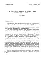
The study of the number of descendants has applications in the context of paged trees (see for
instance [20, 14]). A paged binary search tree with page capacity b stores all its subtrees of size
≤ b (possibly empty) in pages; typically, the pages reside in secondary memory and the elements
within a page are not organized as search trees (see Figure 1: the pagination of the search tree at
the left is indicated using dashed lines; a more “realistic” representation of the same tree appears
at its right).
Let P
(b)
n
be the number of pages in a random search tree of size n with page capacity b.Itis
obvious that P
(b)
n
= I
(b)
n
+ 1, where I
(b)
n
is the number of internal nodes that are the root of a
subtree that contains more than b items. In other words, in a paged search tree, we have external
nodes (pages)thatmaycontainuptobkeys; if P
(b)
n
is the number of external nodes or pages in
a paged search tree, then I

(b)
n
= P
(b)
n
− 1 is the number of internal nodes in the tree, and these
internal nodes are in one-to-one correspondance with the internal nodes with >bdescendants in
the non-paged search tree.
THE ELECTRONIC JOURNAL OF COMBINATORICS 5 (1998), #R20 4
12
7
3
16
12
7
311
915
246
16
14 19
17 20 1, 2 4, 5, 6
9, 11 14 17, 19, 20
Figure 1. A paged binary search tree with page capacity b =3
Proposition 1.4. For all n, and for any constant b ≥ 1,

P
(b)
n

= n

[D
n
>b]+1.
Proof. Let δ
j
be the indicator random variable for the predicate “the j
th
element has more than b
descendants.”. Then I
(b)
n
=

1≤j≤n
δ
j
. The proposition follows taking expectations in both sides
of this equation, because of the linearity of expectations and
[δ
j
]= [D
n,j
>b].
Results about the probabilistic behavior of the number of descendants are also useful in the
analysis of the performance of quicksort if recursive calls are not made on small subfiles (say, of
size ≤ b).
Proposition 1.5. Let C
(b)
n
and R

(b)
n
be the number of comparisons
3
and the number of partitions
made by quicksort to sort n elements, when the recursion halts on subfiles of size ≤ b.Noticethat
standard quicksort corresponds to the case where b =1.Then

R
(b)
n

=n
[D
n
>b],

C
(b)
n

=n(
[D
n
]−1) − n

1≤m≤b
(m −1) [D
n
= m] .

The strategy for the selection of pivots is related with the type of random search trees that we
consider: for BSTs, we have selection of pivots at random; for LBSTs, we have that the pivots are
the medians of random samples of three elements.
Proof. It is well known that we can associate to each particular execution of quicksort a binary
search tree: the root contains the pivot element of the first stage, and the left and right subtrees
are recursively built for the elements smaller and larger than the pivot, respectively. Each internal
node in the search tree corresponds to a recursive call to quicksort. We will make a partitioning of
a given subfile if and only if the subfile contains >belements, i.e. the corresponding internal node
has >bdescendants, and the claim in the proposition follows.
On the other hand, let 
j
be the number of comparisons made between the j
th
element and other
elements, during the partition where the j
th
element was selected as a pivot. Clearly, if D
n,j
≤ b
then 
j
= 0, since no recursive call will be made that chooses the j
th
element as a pivot. On the
other hand, if D
n,j
>b,thej
th
element will be compared with each of its descendants (except
itself) in the associated search tree. Hence,

[
j
]=

n
m=b+1
(m −1) [D
n,j
= m]. We need only to
sum over j to get the desired result.
3
We only count those made during the partitioning phases.
THE ELECTRONIC JOURNAL OF COMBINATORICS 5 (1998), #R20 5
BST LBST
Of a given node Of a random node Of a given node Of a random node
Average [3], Probability, Average [17], Average,
Ascendants
variance
∗
moments, limit variance
∗
variance [27]
∗
,
distribution [23, 5, 22, 18] higher order moments,
PGF, limit distribution
∗
Descendants
Probability, Probability, PGF, average, Probability,
moments [21]

∗
moments [21]
∗
variance
∗
moments
∗
Table 1. Summary of previous works and the results of this paper.
The structure of the paper is as follows. We start with an overview of some basic facts about
generating functions and, in particular, about probability generating functions (Section 2).
In Section 3 we develop the main steps of our approach, taking the analysis of the number of
descendants in random BSTs as a first introductory example. We provide here alternative deriva-
tions to the results of Lent [21], finding the probability that the j
th
node in a random BST of size
n has m descendants (Theorem 3.1). We also find exact and asymptotic values for all ordinary
moments, including the expected value and variance (Theorem 3.2). Then we analyze the number
of descendants of a random node, obtaining the probability that D
n
= m, as well as the moments
of D
n
(Theorems 3.3 and 3.2).
The remaining sections are devoted to the analysis of the number of ascendants and descendants
in random LBSTs. In Section 5 we formally define LBSTs and give an equivalent characterization
of the model of randomness which is more suitable to our purposes.
Among our new results, in Section 6 we derive an explicit form for the generating function of the
probability distribution of D
n,j
(Theorem 6.1) and closed formulæ for the average (Theorem 6.2)

and the second factorial moment (Theorem 6.3). Moreover, we find the probability distribution of
D
n
(Theorem 6.4) and all its moments (Theorem 6.5).
In Section 7, we compute
[A
n,j
], the average number of ascendants of the j
th
node in a random
LBST of size n (Theorem 7.1). We are also able to compute the PGF of A
n
,thenumberof
ascendants of a random node (Theorem 7.2), as well as all its moments (Theorems 7.4 and 7.5),
thus extending the results of Poblete and Munro [27].
The results of previous works and the new results in this paper are summarized in Table 1.
Entries corresponding to new results in this paper and to alternative derivations of previous results
are marked by ‘
∗
’.
2. Mathematical Preliminaries
We start recalling the definition of generating function, for the reader’s convenience. Given a
sequence {a
n
}
n≥0
its generating function A(z) is the formal power series
A(z)=

n≥0

a
n
z
n
.
As usual, [z
n
]A(z) denotes the coefficient of z
n
in A(z) (the n
th
coefficient of A(z)). Excellent
sources of information about generating functions and their applications to combinatorics and the
analysis of algorithms are [35, 33, 32, 20].
We make extensive use in this paper of probability generating functions (PGFs) as well as
multivariate generating functions whose coefficients are PGFs themselves. We define them in turn.
Given a discrete random variable X, its probability generating function X(z)is
X(z)=

m
[X=m]z
m
.
THE ELECTRONIC JOURNAL OF COMBINATORICS 5 (1998), #R20 6
If we assume further that X ≥ 0andletp
m
= [X=m], the PGF of the random variable X is
nothing but the ordinary generating function of the sequence {p
m
}

m≥0
. We list now a few important,
although elementary, properties of PGFs.
Proposition 2.1. For any discrete random variable X, its probability generating function X(z)
satisfies:
1. X(1) = 1.
2. X

(1) =
dX
dz




z=1
= [X].
3. X
(s)
(1) =
d
s
X
dz
s




z=1

= [X
s
], where X
s
denotes the s
th
falling factorial of X,thatis,X
s
=
X(X−1) (X −s+1).Thequantity
[X
s
]is customarily called the s
th
factorial moment
of the random variable X. Ordinary and central moments may be recovered from factorial
moments quite easily. For instance, if µ =
[X], the variance of X is given by
[X]=

(X−µ)
2

=

X
2

+
[X]− [X]

2
.
Since we will mostly deal with families of random variables, with two (n and j)orone(n) index,
we will systematically work with multivariate generating functions of these families. For instance, if
we were interested in the family {X
n,j
}
1≤j≤n
, we would introduce a generating function X(z,u, v)
in three variables, such that the coefficient of z
n
u
j
v
m
in X(z,u, v) is the probability that X
n,j
is
m.Thus
X(z,u,v)=

n,j,m
[X
n,j
= m] z
n
u
j
v
m

, (1)
where the indices of summation n, j and m run in the appropriate ranges (or we assume that
[X
n,j
= m] is 0 whenever n<1, j<1, j>nor m<0). Notice that, by definition, [z
n
u
j
]X(z,u,v)
is the PGF of the random variable X
n,j
,and[z
n
u
j
v
m
]X(z,u,v)= [X
n,j
= m].
For technical reasons that will be clearer later, we will also use sometimes the derivative w.r.t. z
of such a multivariate generating function. We will introduce then
X
z
(z,u,v)=
∂
∂z

n,j,m
[X

n,j
= m] z
n
u
j
v
m
=

n,j,m
n [X
n,j
= m] z
n−1
u
j
v
m
rather than the more natural definition given in Equation (1). This means that once we were able
to extract coefficients from such a generating function, let us say the coefficient of z
n−1
u
j
v
m
,we
must divide by n to obtain
[X
n,j
= m].

Furthermore, we are also interested in investigating all the moments of the random variables:
mean, variance, and higher order moments. We differentiate the generating function X(z,u,v)
s times with respect to v and let v = 1, to get the generating function for the s
th
factorial moments,
i.e.
X
(s)
(z,u)=
∂
s
X(z, u,v)
∂v
s




v=1
,s≥1. (2)
Recall that [z
n
u
j
]X
(s)
(z,u)=

X
s

n,j

.
Grand averages correspond to the situation where the rank —the parameter j in X
n,j
—is
random itself. More precisely, let X
n
≡ X
n,Z
n
, where Z
n
is a uniformly distributed random variable
THE ELECTRONIC JOURNAL OF COMBINATORICS 5 (1998), #R20 7
in {1, ,n}.ThenX
n
is the grand average of the random variables X
n,1
, ,X
n,n
. It follows that
[X
n
= m]=
1
n

1≤j≤n
[X

n,j
= m] . (3)
We remark that X
n
=
1
n
(X
n,1
+ ···+X
n,n
), even if the X
n,j
’s are independent.
Unless we are dealing with a differentiated version of the generating function X(z,u,v), we have
X(z, v)=X(z, 1,v)=

n,m
z
n
v
m

1≤j≤n
[X
n,j
= m] . (4)
Thus the coefficient [z
n
v

m
]X(z,v), divided by n, is the probability that X
n
is m.Inthecase
that X
z
(z,u,v) were a differentiated generating function, then we should divide the coefficient
[z
n−1
v
m
]X
z
(z,v)byn
2
. Finally, computing the derivatives of X(z,v) w.r.t. v and setting v =1
yields the generating functions for the factorial moments of the grand average X
n
.
The main steps of the systematic procedure that we will follow are thus:
1. Set up a recurrence for
[X
n,j
= m];
2. Translate the recurrence to a functional equation over the corresponding generating function
X(z,u,v);
3. Solve the functional equation;
4. Extract the coefficients of X(z, u, v);
5. Repeatedly differentiate X(z,u,v) w.r.t. v and set v = 1; extract the coefficients to get the
factorial moments of X

n,j
;
6. Set
X(z, v)=X(z,1,v) and repeat steps 4 and 5 for X(z,v).
In practice, the procedure might fail for several reasons. Typically, because we are not able to
solve the equation at step 3 or to extract the coefficients of a given generating function. Although
we have (almost) not used them in this paper, the reader should be aware of the existing powerful
techniques to extract asymptotic information about the coefficients of a generating function if we
know its behaviour near its singularities or in some case, even if we only know the functional
equation satisfied by the generating function [33, 6]. Also, if we are not able to solve and get an
explicit form for X(z,u,v), we can still differentiate w.r.t. to v or set u = 1 and try to solve the
(easier) resulting differential equations, to get information about the moments or the grand average.
The functional equations that arise in our study are linear partial differential equations of the
first (BSTs) and of the second (LBSTs) order. The former can be solved, in principle, by quadrature
through the variation of constant —actually, functions in u and v— method. For the second order
differential equations, the theory of hypergeometric differential equations comes into play [16].
Nowadays, most of the necessary mathematical knowledge is embodied into modern computer
algebra systems. In our case, Maple needed little or no assistance to solve the differential equations
that we had.
The last step, that of extracting coefficients in exact form, was, at large, the least systematic
and mechanical one. A great deal of combinatorial identities, inspired guessing and patience was
needed. Standard Maple tools like the function interp or the Gfun package [29] proved also to be
useful. However,
once the solution is obtained, it is just a matter of minutes to check its correctness. It is quite
difficult to provide a detailed and ordered description of the methods that we used to extract
coefficients from generating functions. As a result, the paper contains only some hints here and
there, while some claims are just stated without further explanation.
THE ELECTRONIC JOURNAL OF COMBINATORICS 5 (1998), #R20 8
3. The number of descendants in random BSTs
The number of the descendants D

n,j
of the j
th
node of a BST of size n is recursively computed
as the number of descendants in the left subtree of the j
th
node, plus the number of descendants in
its right subtree, plus one (to count the j
th
node itself). The probability that D
n,j
= m is computed
conditioning on the events “the rank of the root is k,” that means the root is the k
th
node of a
search tree. Recall that, for a random BST of size n, the rank of the root is k with probability 1/n,
for k =1, ,n. Using the recursive definition of D
n,j
we have
[D
n,j
= m]=
n

k=1

D
n,j
= m |therootisthek
th

element

×

therootisthek
th
element

=
1
n
[[ m = n ]] +
1
n
j − 1

k =1
[D
n−k,j−k
= m]+
1
n
n

k=j+1
[D
k−1,j
= m] , (5)
where [[P]] i s 1 i f P is true and 0 otherwise [10].
This recursion translates nicely into a functional equation over the generating function for the

family of random variables {D
n,j
}. Solving the functional equation and extracting coefficients of
the generating function, we get the following theorem, which was already found by Lent [21] using
probabilistic techniques.
Theorem 3.1. The probability that the j
th
internal node of a random binary search tree of size
n has m descendants is, assuming that j ≤ n +1−j,
[D
n,j
= m]=






















2
(m+1)(m+2)
for 1 ≤ m<j,
1
(m+1)(m+2)

1+
2j
m

for j ≤ m<n+1−j,
2(n +1)
m(m+1)(m+2)
for n +1−j ≤m<n,
1
n
for m = n.
For the cases where j>n+1−j we can use the symmetry on j and n +1−j (Proposition 1.1)
to compute the corresponding probabilities.
Also, the distribution function for D
n,j
is
[D
n,j
≤ m]=


















m
m+2
for 1 ≤ m<j,
m+1
m+2
−
j
(m+1)(m+2)
for j ≤ m<n+1−j,
m
2
+3m+1−n
(m+1)(m+2)
for n +1−j≤m<n,
1 for m = n.

Proof. We start defining the generating function
D(z,u,v)=

1≤j,m≤n
[D
n,j
= m] z
n
u
j
v
m
.
THE ELECTRONIC JOURNAL OF COMBINATORICS 5 (1998), #R20 9
Multiplying both sides of (5) by nz
n−1
u
j
v
m
and summing for all n ≥ 1, 1 ≤ j ≤ n and m ≥ 1,
yields
∂D
∂z
=
uD
1 −uz
+
D
1 − z

+
uv
(1 − vz)(1 −uvz)
,
D(0,u,v)=0. (6)
The solution to the differential equation above is relatively simple
D(z, u,v)=
uz
v(1 −z)(1 −uz)
−
u(1 −v)(v − u)
(1 − z)(1 −uz)v
2
(1 − u)
log
1
1 − vz
−
(1 − v)(1 − uv)
(1 − z)(1 −uz)v
2
(1 − u)
log
1
1 − uvz
. (7)
The statement of the theorem follows after extracting the coefficient [z
n
u
j

v
m
]D(z, u, v).
The explicit and simple form of the trivariate generating function in Theorem 3.1 allows us to
computeallthemomentsexplicitly. It is convenient to deal with a sort of shifted factorial moments;
the ordinary moments can be computed by linear combinations of the shifted factorial ones.
Theorem 3.2. Let d
(s)
n,j
= [(D
n,j
+2)
s
] and d
n,j
= d
(1)
n,j
, where D
n,j
denotes the number of
descendants of the j
th
internal node in a random binary search tree of size n. For all n>0and all
1 ≤ j ≤ n,
1. d
n,j
= H
j
+ H

n+1−j
+1,
2. d
(2)
n,j
=2(n+1)H
n
−2jH
j
−2(n +1−j)H
n+1−j
+2(n+2).
3. For all s ≥ 3,
d
(s)
n,j
=
s
s − 2
(n +1)
s−1
−
s
(s−1)(s − 2)

j
s−1
+(n+1−j)
s−1


.
Proof. We begin by introducing
D
(s)
(z,u)=
∂
s
(v
2
D(z, u,v))
∂v
s




v=1
,
and hence its coefficients are
d
(s)
n,j
=[z
n
u
j
]D
(s)
(z,u)= [(D
n,j

+2)
s
].
The shifted moments are particularly easy to obtain, since the coefficients of D
(s)
(z,u) that we seek
are linear combinations of the coefficients of the next generating functions:
∂
s
∂v
s
log
1
1 − vz



v=1
=(s−1)!

z
1 − z

s
,
∂
s
∂v
s
v log

1
1 − vz



v=1
=(s−1)!

z
1 − z

s
+ s(s −2)!

z
1 − z

s−1
,
∂
s
∂v
s
v
2
log
1
1 − vz




v=1
=(s−1)!

z
1 − z

s
+2s(s−2)!

z
1 − z

s−1
+ s(s −1)(s − 3)!

z
1 − z

s−2
,
∂
s
∂v
s
log
1
1 − uvz




v=1
=(s−1)!

uz
1 − uz

s
,
THE ELECTRONIC JOURNAL OF COMBINATORICS 5 (1998), #R20 10
∂
s
∂v
s
v log
1
1 − uvz



v=1
=(s−1)!

uz
1 − uz

s
+ s(s −2)!

uz

1 − z

s−1
,
∂
s
∂v
s
v
2
log
1
1 − uvz



v=1
=(s−1)!

uz
1 − uz

s
+2s(s−2)!

uz
1 − uz

s−1
+ s(s −1)(s −3)!


uz
1 − uz

s−2
.
We might additionally observe that for all n ≥ 0and1≤j≤n
[z
n
u
j
]
1
(1 − z)
s+1
(1 − uz)(1 −u)
=

s + n +1
s+1

−

s+n−j
s+1

,
[z
n
u

j
]
1
(1 − z)(1 −uz)
s+1
(1 − u)
=

s + j +1
s+1

, and
[z
n
u
j
]
1
(1 − z)
2
(1 − uz)
2
=(j+1)(n+1−j).
Theorem 3.2 is an immediate consequence of the formulæ above.
Corollary 3.1. The expected value and variance of D
n,j
are, respectively,
[D
n,j
]=H

j
+H
n+1−j
− 1,
[D
n,j
]=2(n+1)H
n
−(2j +1)H
j
−(2n − 2j +3)H
n+1−j
+2(n+2)−H
2
j
−H
2
n+1−j
− 2H
j
H
n+1−j
.
Furthermore, for j = αn,with0<α<1,wehave
[D
n,αn
]=2logn+logα+log(1−α)+2γ−1+o(1),
[D
n,αn
]=2n


1−αlog α − (1 −α)log(1−α)

+
O
(log
2
n),
where γ =0.5772156649 is Euler’s constant.
To recover higher order ordinary moments, we only need to express the ordinary powers as linear
combinations of the shifted falling factorials with coefficients λ
s,k
.Thus
x
s
=
s

k=0
λ
s,k
(x +2)
k
.
It is easy to show that
λ
s,k
=
s


i=k

i
k

s
i

(−2)
s−i
,
where

i
k

denote Stirling numbers of the second kind. The coefficients λ
s,k
satisfy a recursion that
is similar to that of the Stirling numbers
λ
s+1,k
= λ
s,k−1
+(k−2)λ
s,k
,
and λ
s,0
=(−2)

s
.
Let us consider now D
n
, the number of descendants of a random node in a random BST of size
n. The following two theorems give closed formulæ for the probability that D
n
is m and for the
shifted factorial moments of D
n
, i.e. for d
(s)
n
= [(D
n
+2)
s
].
THE ELECTRONIC JOURNAL OF COMBINATORICS 5 (1998), #R20 11
Theorem 3.3. The probability that a randomly chosen internal node in a random binary search
tree of size n has m descendants is given by
[D
n
= m]=





2(n +1)

n(m+1)(m+2)
for 1 ≤ m<n,
1
n
for m = n.
Proof. Plug u = 1 into the solution of (7) to get
D(z,v)=D(z, 1,v)=−
2(1 −v)
v
2
(1 − z)
2
log
1
1 − vz
−
z(zv −v
2
+2v−2)
v(1 −vz)(1 −z)
2
. (8)
The coefficient of [z
n
v
m
]D(z,v), divided by n, is the sought probability.
Theorem 3.4. The s
th
shifted factorial moment d

(s)
n
= [(D
n
+2)
s
]of the number of descendants
of a random node in a random binary search tree of size n is given by
1. d
n
= d
(1)
n
=2(1+
1
n
)H
n
−1,
2. d
(2)
n
=3(n+1).
3. For all s ≥ 3,
d
(s)
n
=
1
n


(n +2)
s
+
2
s−1
(n+1)
s

∼
s+1
s−1
n
s−1
.
Proof. Repeated differentiation of the generating function v
2
D(z,v) w.r.t. v and setting v =1,gives
us the generating functions of the shifted factorial moments. Their coefficients are extracted much
in the same way as in Theorem 3.2.
A few comments concerning the last theorem are in order now. Observe that for s ≥ 3
1
n
n

j=1
d
(s)
n,j
=

(n +1)
s−1
s−1

s+1+
2
n

.
Asymptotically, this quantity is
∼
s +1
s−1
n
s−1
,
one of the observations in the work of Lent [21]. The coincidence in asymptotic behavior with d
(s)
n
is remarkable; recall that in general
[D
s
n
] =



1
n


1≤j≤n
D
n,j

s


,
except when s = 1 and the same observation holds for the shifted factorial moments we were dealing
with.
Last, but not least, we can obtain the following corollaries, from Propositions 1.4 and 1.5 and
the theorems in this section. These results can already be found in [20], although there is a slight
difference in

C
(b)
n

, because n + 1 comparisons per partition are counted there, while we count
n − 1 comparison per partition.
Corollary 3.2. The expected number of pages in a random binary search tree of size n with page
capacity b is

P
(b)
n

=2
n+1
b+2

.
THE ELECTRONIC JOURNAL OF COMBINATORICS 5 (1998), #R20 12
The filling ratio for binary search trees is thus
γ
b
=
n/b

P
(b)
n

∼
1
2
.
Corollary 3.3. The expected number of recursive calls to sort a random permutation of size n,
when the recursion stops in subfiles of size ≤ b is

R
(b)
n

=
2n − b
b +2
.
Also, the expected number of comparisons to sort a random permutation of size n, when the
recursion stops in subfiles of size ≤ b is


C
(b)
n

=2(n+1)(H
n
−H
b+1
)+n+5−
6(n +1)
b+2
.
4. The number of ascendants in random BSTs
Considering the element k of the root of a BST, we obtain for the number of ascendants A
n,j
of
the j
th
node of a BST of size n the following recursion:
[A
n,j
= m]=
1
n
[[ m =1]]+
1
n
j−1

k=1

[A
n−k,j−k
= m −1] +
1
n
n

k=j+1
[A
k−1,j
= m −1] . (9)
Introducing the generating function for the family of random variables {A
n,j
}
A(z,u,v)=

1≤j,m≤n
[A
n,j
= m] z
n
u
j
v
m
,
this recursion translates by multiplying both sides by nz
n−1
u
j

v
m
and summing for all n ≥ 1,
1 ≤ j ≤ n and m ≥ 1 into the following differential equation:
∂A
∂z
=
v
1 −z
A +
uv
1 − uz
A +
uv
(1 − z)(1 −uz)
with the initial condition A(0,u,v) = 0. This differential equation has the following solution
A(z, u,v)=
uv
(1 − z)
v
(1 − uz)
v

z
0
(1 − t)
v−1
(1 − ut)
v−1
dt. (10)

Starting with this generating function, it is easy to get the following theorems. At first we obtain
an old result from [3]:
Theorem 4.1. The expected number of ascendants a
n,j
= [A
n,j
] of the j
th
node in a random
binary search tree of size n is
a
n,j
= H
j
+ H
n+1−j
− 1.
Proof. Starting with (10), taking derivatives w.r.t. v and setting v = 1, we get the generating
function A(z, u), whose coefficients are the expected values a
n,j
= [A
n,j
]. It is given by
A(z, u)=
u
(1 − z)(1 −uz)
log
1
1 − z
+

1
(1 − z)(1 −uz)
log
1
1 − uz
−
uz
(1 − z)(1 −uz)
.
It is easy to extract the coefficients of this expression, which leads immediately to the stated
theorem.
THE ELECTRONIC JOURNAL OF COMBINATORICS 5 (1998), #R20 13
Theorem 4.2. The second factorial moment a
(2)
n,j
=

(A
n,j
)
2

of the number of ascendants of
the j
th
node in a random binary search tree of size n is
a
(2)
n,j
=

2(n+1)
(n+1−j)j
H
n
+H
2
j
+2H
j
H
n+1−j
+
2

−nj − n + j
2
−j − 1

(n +1−j)j
H
j
+H
2
n+1−j
+
2

−nj − n + j
2
− j −1


(n +1−j)j
H
n+1−j
− H
(2)
j
− H
(2)
n+1−j
−
2(−2 nj +2j
2
−2j−1)
(n +1−j)j
.
(11)
Proof. Differentiating equation (10) two times w.r.t. v and setting v = 1 gives the generating
function A
(2)
(z,u) of the second factorial moments a
(2)
n,j
of the number of ascendants:
A
(2)
(z,u)=−
2zu
(1 − uz)(1−z)
log

1
1 − uz
−
2zu
(1 −uz)(1−z)
log
1
1 − z
−
2(uz − u −1)
(1 − uz)(1−z)
log
1
1 − z
log
1
1 − uz
+
u
(1 − uz)(1−z)
log
2
1
1 − z
+
1
(1 − uz)(1−z)
log
2
1

1 − uz
+
2u
(1 − uz)(1−z)

z
0
log
1
1 − t
log
1
1 − ut
dt.
Extracting the coefficients leads to the given theorem. Since one expression in A
(2)
(z,u) turns out
to be a bit messier, we sketch how to extract the coefficients of it. First we get the following sum
[z
n
u
j
]
1
(1 − z)(1 −uz)

z
0
log
1

1 − t
log
1
1 − ut
dt =
j

k=0
n−j+k

l=0
[z
l
u
k
]

z
0
log
1
1 − t
log
1
1 − ut
dt
=
j

k=1

n−j+k

l=k+2
1
lk(l −k −1)
,
which can be simplified to
j

k=1
n−j+k

l=k+2
1
lk(l −k −1)
=
j

k=1
1
k
n−j−1

l=1
1
l(l + k +1)
=
j

k=1

1
k(k +1)
n−j−1

l=1

1
l
−
1
l + k +1

=
j

k=1
1
k(k +1)
(H
n−j−1
+H
k+1
− H
n−j+k
)=
j

k=1

1

k
−
1
k +1

(H
n−j−1
+H
k+1
− H
n−j+k
)
= H
n−j−1
j

k=1

1
k
−
1
k +1

+
j

k=1

H

k
k
−
H
k+1
k +1

+
j

k=1

1
k
−
1
k +1

−
j

k=1

H
n−j+k
k
−
H
n−j+k+1
k +1


−
1
n−j
j

k=1

1
k +1
−
1
n−j+k+1

.
The sums telescope and we finally get
[z
n
u
j
]
1
(1 − z)(1 −uz)

z
0
log
1
1 − t
log

1
1 − ut
dt =
n +1
(j+1)(n−j)
(H
n+1
− H
j+1
− H
n+1−j
)
+
2jn
2
−4nj
2
+2j
3
+n
2
−jn +2n−2j+1
(n−j)(j +1)(n+1−j)
.
The next theorem gives the variance, which is now easy to obtain.
THE ELECTRONIC JOURNAL OF COMBINATORICS 5 (1998), #R20 14
the insertion hits
one of these leaves
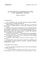
Figure 2. The fringe heuristic
Theorem 4.3. The variance

[A
n,j
] of the number of ascendants of the j
th
node in a random
search tree of size n is
[A
n,j
]=
2(n+1)
(n+1−j)j
H
n
+

nj − 2 n −j
2
+ j −2

(n +1−j)j
H
j
+

nj − 2 n −j
2
+ j − 2

(n +1−j)j
H

n+1−j
− H
(2)
j
− H
(2)
n+1−j
+
2(nj − j
2
+ j +1)
(n+1−j)j
.
(12)
5. Locally balanced binary search trees
One approach to avoid drastically unbalanced binary search trees is the introduction of strict
balance constraints like in AVLs or red-black trees [1, 11]. Such schemes guarantee logarithmic
performance of searches and updates in the worst-case, but they have additional space requirements
and are more difficult to implement than standard BSTs. As an alternative, several authors [4, 34,
27] have suggested the use of a simple heuristic that makes the construction of poorly balanced
trees much less likely than with the use of the standard algorithms. Furthermore, the heuristic was
shown to yield significant savings in the expected search time.
The basic idea is really simple: whenever a son is appended to a node that itself is a single
son (its “brother” is an external node), a rotation of the three nodes is performed to place the
median of the three elements as the root of the subtree and the other two elements as sons (see
Figure 2). Since no other kind of rebalancing operation is ever made, Poblete and Munro refer to
this technique as a fringe heuristic. We will call the binary search trees constructed in this way
local ly balanced binary search trees (LBST, for short).
Poblete and Munro [27] and Poblete [26] carry on the analysis of this heuristic and some gener-
alizations by means of bottom-up or fringe techniques: they basically study the number of nodes

that are at level k and which are the root of a subtree of size 1 or 2.
As we have already mentioned in the introduction, the standard model for random LBSTs states
that a random LBST of size n is the result of n random insertions into an initially empty tree.
Equivalently, a random LBST of size n is the result of inserting the elements of a random permuta-
tion of {1, ,n}into an initially empty tree. Here, we show that a recursive, top-down definition
of the randomness model is also possible. This characterization of the model of randomness is more
amenable to the kind of algebraic manipulations that we want to carry on; as we will see, the
recurrence relations for the analyzed quantities translate to equations over generating functions in
a natural way, almost automatically.
THE ELECTRONIC JOURNAL OF COMBINATORICS 5 (1998), #R20 15
Definition 5.1. 1. A random binary search tree of size s ≤ 2 is also a random locally balanced
search tree. Recall that a BST of size 2 is random if the smallest (resp. largest) key is the root
with probability 1/2.
2. A binary search tree T of size n ≥ 3, with left and right subtrees T
1
and T
2
, is a random
LBST if and only if, both T
1
and T
2
are random independent LBSTs, and
π
n,k
=

|T
1
| = k − 1




|T | = n

=
(k −1)(n −k)

n
3

, for all 1 ≤ k ≤ n.
The reader should have noticed that the only difference between this definition and that for
random BSTs relies on the splitting probabilities π
n,k
. In the case of BSTs, each element of the
random permutation has the same probability (namely, 1/n) of being the first element and hence
of becoming the root. In the case of LBSTs, when n ≥ 3, the probability that the k
th
element is
one of the first three elements of the permutation and is the median of these three elements is
1
n
×
k − 1
n − 1
×
n − k
n − 2
× 3! = π

n,k
.
Indeed, the left hand side of the equation above give us the probability that the k
th
element is
the first, times the probability that it is followed by a smaller element, times the probability that
the two elements are followed by a larger element. For any permutation of such three elements,
we have that the k
th
element is among the first three elements and it is their median. Now, under
these conditions the k
th
element will be the root of the LBST (after the insertion of the first three
elements, with rebalancing if necessary). The insertion of the fourth, fifth, etc. elements will not
affect the root of the LBST. The principle applies recursively to the subsequences of elements
smaller and greater than the selected element and the definition follows.
This argument also justifies the deep connection between LBSTs, quicksort and quickselect (see
Propositions 1.3 and 1.5), when we consider the variants that select the median of 3 elements taken
at random as the pivot of each partitioning phase.
6. The number of descendants in random LBSTs
As in Section 3, let D
n,j
denote the number of descendants of the j
th
node, but now in a random
LBST of size n. The recursion for
[D
n,j
= m] is almost the same as for random BSTs, the only
difference being the splitting probability π

n,k
, the probability that the root of the LBST is the k
th
element. Thus,
[D
n,j
= m]=


1≤k<j
π
n,k
[D
n−k,j−k
= m]+π
n,j
[[ m = n ]]
+

j<k≤n
π
n,k
[D
k−1,j
= m]

. (13)
Theorem 6.1. Let
D
z

(z,u,v)=
∂
∂z

n,j,m
[D
n,j
= m] z
n
u
j
v
m
=

n,j,m
n [D
n,j
= m] z
n−1
u
j
v
m
.
Then,
D
z
(z,u,v)=
A

0
(z, u, v)
v(1 − z)
2
(1 − uz)
2
(1 − uv)
2
(1 − v)
2
(v − u)
2
(1 − u)
2
+
A
1
(z,u,v)
(1 − uz)
2
(1 − u)(1 − v)
3
(1 − uv)
3
log
1
1 − z
+
A
2

(z,u,v)
(1 − z)
2
(u −v)
3
(1 − u)(1 − v)
3
log
1
1 − uz
THE ELECTRONIC JOURNAL OF COMBINATORICS 5 (1998), #R20 16
+
A
3
(z,u,v)
v
2
(1 − z)
2
(1 − uz)
2
(v − u)
3
(1 − u)
3
(1 − v)
3
log
1
1 − vz

+
A
4
(z,u,v)
v
2
(1 − z)
2
(1 − uz)
2
(1 − u)
3
(1 − v)
3
(1 − uv)
3
log
1
1 − uvz
,
where each of the A
i
(z,u,v)’s is a complicated polynomial in z, u and v. They are listed in full in
the appendix.
Proof. We multiply the recursion (13) by

n
3

and z

n−3
u
j
v
m
, sum up over all n ≥ 1and1≤j, m ≤ n
to get the following differential equation:
1
6
∂
2
D
z
∂z
2
=
u
2
v
3
(1 − vz)
2
(1 − uvz)
2
+
u
2
(1 − uz)
2
D

z
+
1
(1 − z)
2
D
z
, (14)
where the initial conditions are D
z
(0,u,v)=uv and
∂
∂z
D
z
(0,u,v)=uv(1 + u)(1 + v). We use the
partial derivative w.r.t. z to define D
z
(z,u,v) because the differential equation just given, which
translates the recurrence for
[D
n,j
= m], is then of the second order. Had we introduced the
generating function D
z
(z,u,v) in the standard manner, we would have had a third order differential
equation, with no appearance of the function itself, only the first and third derivatives.
The differential equation (14) is solvable: its explicit form (abridged) is the one given in the
statement of the theorem.
From the explicit form of D

z
(z,u,v) given in Theorem 6.1 we can, in principle, compute exact
expressions for
[D
n,j
= m] and all moments. However, the task is daunting, and we will content
ourselves computing the expected value and the second factorial moment in the next two theorems.
Theorem 6.2. The expected number of descendants d
n,j
= [D
n,j
] of the j
th
node in a random
LBST of size n is, when 5 ≤ j ≤ n −4
d
n,j
= −
12
7
H
n
+
12
7
H
j
+
12
7

H
n+1−j
−
6
7j
−
6
7(n +1−j)
+
79
70
−
3(3j − 5)
7n
+
6(j − 1)
2
7n
2
+
2(2j − 3)(j − 1)
2
7n
3
+
3(j − 2)(j − 1)
3
7n
4
−

3(2j − 5)(j − 1)
4
7n
5
+
2(j − 3)(j − 1)
5
7n
6
.
The remaining cases when j ≤ 4 (or when j>n−4, by symmetry) appear in the appendix.
Proof. Taking the first derivative with respect to v, and setting v =1weget
4
∂D
z
∂v




v=1
=
B
0
(z,u)
70(1 −uz)
2
(1 − u)
7
(1 − z)

2
+
B
1
(z,u)
7(1 −u)
7
(1 − uz)
2
log
1
1 − z
+
B
2
(z,u)
7(1 −z)
2
(1 − u)
7
log
1
1 − uz
,
where the B
i
(z,u)’s are polynomials in z and u. Their explicit value can be found in the appendix
at the end of this paper.
4
It turns out that Maple gets stuck doing the work in the obvious way, i.e. take the derivative, then take the limit

when v → 1. But we can produce the differential equations satisfied by the generating functions for the factorial
moments from the differential equation (14) and solve them. Also, the problem can be fixed by computing a series
expansion of the derivatives around v =1.
THE ELECTRONIC JOURNAL OF COMBINATORICS 5 (1998), #R20 17
In order to get to the coefficients, we use formulæ such as
[z
n
u
j
]
1
(1 − u)
4
(1 − uz)
2
log
1
1 − z
=(n+1)

j−n+3
3


H
n
−H
n−1−j

+

(j+1)n
3
6
−
5(j +1)(j+2)n
2
12
+
(j + 1)(11j
2
+40j+ 30)n
36
−
3j − 10
12

j +3
3

,
[z
n
u
j
]
1
(1 − u)
5
(1 − uz)
2

log
1
1 − z
=(n+1)

j−n+4
4


H
n
−H
n−1−j

−
(j+1)n
4
24
+
(7j + 18)(j +1)n
3
48
−
(j + 1)(13j
2
+65j+ 75)n
2
72
+
(j + 1)(25j

3
+ 173j
2
+ 348j + 180)n
288
−
12j − 65
60

j +4
4

,
and similar ones that are not too hard to obtain. To retrieve the final answer, we have also to take
into account that we need to shift the coefficients in z
n
by 1 and multiply by
1
n
, because we were
considering
∂
∂z

n,j,m
[D
n,j
= m] z
n
u

j
v
m
. Putting everything together, the theorem follows.
Theorem 6.3. The second factorial moment of the number of descendants d
(2)
n,j
=

D
2
n,j

of the
j
th
node in a random LBST of size n is, when 5 ≤ j ≤ n − 4,
d
(2)
n,j
=

36n
5
−
12
35

H
n

+

36j
5
−
36n
5
−
48
7

H
n+1−j
+

12
35
−
36j
5

H
j
−
132
35j
−
132
35(n +1−j)
+

3489
175
−
33j
5
+

66
7
−
429j
35
+
33j
2
5

1
n
+
132(j − 1)
2
35n
2
+
44(2j − 3)(j −1)
2
35n
3
+

66(j − 2)(j − 1)
3
35n
4
−
66(2j − 5)(j − 1)
4
35n
5
+
44(j − 3)(j − 1)
5
35n
6
.
The formulæ for the second factorial moment in the special cases (when j ≤ 4 or j>n−4)are
collected in a table in the appendix.
Proof. The second factorial moment d
(2)
n,j
is the coefficient of z
n−1
u
j
times
1
n
in
∂
2

D
z
∂v
2




v=1
=
C
0
(z,u)
35(1 −z)
2
(1 − u)
7
(1 − uz)
2
+
C
1
(z,u)
35(1 −z)
2
(1 − u)
7
(1 − uz)
2
log

1
1 − z
+
C
2
(z,u)
35(1 −z)
2
(1 − u)
7
(1 − uz)
2
log
1
1 − uz
where the C
i
(z,u)’s are polynomials in z and u. They have been listed in the appendix. Using
techniques similar to the ones in the proof of Theorem 6.2, we extract the coefficients and obtain
the stated result.
THE ELECTRONIC JOURNAL OF COMBINATORICS 5 (1998), #R20 18
As in Section 3, we shift now our attention to the number of descendants of a random node in
a random LBST of size n. We start giving an explicit expression for the probability distribution of
D
n
.
Theorem 6.4. The probability that a random node in a random LBST of size n has m descendants
is
[D
n

= m]=
12
7
(n +2+m)(n −1 − m)
n
2
(m +1)(m+2)
−
12
7
m
5
nn
6
+
12
7n
2
,
for 5 ≤ m<n. The probability that a random node has n descendants is
[D
n
= n]=
1
n
.
Furthermore, the probability that a random node in a random LBST of size n has no children is
[D
n
=1]=

6
7
1
n
2

n+1
2

=
3
7

1+
1
n

.
In the appendix, a table collects the general result for 5 ≤ m<nas well as the special cases
where m<5or m = n.
Proof. If we consider the explicit form for D
z
(z,u,v) given in Theorem 6.1 and average w.r.t. j, i.e.
we plug u = 1 there, we get
D
z
(z,v)=
v
(1 − vz)
2

+
12
7(1 − v)(1 −z)
−
24
7v(1 −z)
2
+
2(v
2
− 6v + 12)
7v(1 −z)
3
+
v
7(1 −v)
5

− 15(1 −v)
3
+20v(1 − v)
2
(1 − z) −30v
2
(1 − v)(1 −z)
2
+60v
3
(1 − z)
3

+(1−7v+23v
2
−57v
3
− 22v
4
+2v
5
)(1 − z)
4

−
60
7
v
5
(1 − z)
4
(1 − v)
6
log
1
1 − z
+

60
7
v
5
(1 − z)

4
(1 − v)
6
−
24
7
1 −v
v
2
(1 − z)
3

log
1
1 − vz
. (15)
Alternatively, we can write down the differential equation for
D
z
(z,v)=D
z
(z, 1,v)andsolveit.
The differential equation is
1
6
∂
2
D
z
∂z

2
=
v
3
(1 − vz)
4
+2
D
z
(1 −z)
2
,
where the initial conditions are
D
z
(0,v)=v,and
∂
∂z
D
z
(0,v)=2v(1 + v). The reader may readily
check that the explicit form given in Equation (15) is a solution to the differential equation above.
The purely rational term in Equation (15), i.e. the one that is not multiplied by any logarithmic
function, although more complicated than the others, has the very pleasant feature that “almost”
all coefficients are
12
7
. On the other hand,
[z
n

v
m
]
1
(1 − z)
3
log
1
1 − vz
=
1
m

n −m +2
2

,
and thus
−[z
n
v
m
]
24
7
1 − v
v
2
1
(1 − z)

3
log
1
1 − vz
=
12
7
(n +3+m)(n −m)
(m +2)(m+1)
.
This is the main contribution in the coefficient z
n
v
m
of D
z
(z,v), the remaining contributions being
small. Indeed,
60
7
v
5
(1 − z)
4
(1 − v)
6
log
1
1 − vz
produces no coefficients at all, since m ≤ n. And the remaining contribution comes from

−[z
n
v
m
]
60
7
v
5
(1 − z)
4
(1 − v)
6
log
1
1 − z
= −
12
7
m
5
n
5
.
THE ELECTRONIC JOURNAL OF COMBINATORICS 5 (1998), #R20 19
The general part of the theorem follows from the considerations made above. The special cases,
when m<5orm=nhave to be dealt with separately. In particular, to get the probability that a
random node in a random LBST of size n has no children (the special case m =1)wecompute
∂
D

z
(z, v)
∂v




v=0
=
6
7
1
(1 − z)
3
+
1
7
(1 − z)
4
,
extract the coefficient of z
n−1
in the GF above and divide by n
2
, yielding [D
n
=1]∼3/7. Also,
for evident reasons,
[D
n

= n]=1/n, since only the root has n descendants and we choose it with
probability 1/n.
Finally, the moments of D
n
can be computed after differentiation of D
z
(z,v), whose explicit form
was given in the proof above. We state now the following result.
Theorem 6.5. Let d
(s)
n
= [(D
n
+2)
s
], i.e., d
(s)
n
is the shifted s
th
factorial moment of the num-
ber of descendants of a random node in a random locally balanced binary search tree of size n.
Furthermore, let d
n
= d
(1)
n
.Then
1. d
n

=
12
7

1+
1
n

H
n
−
1
49

26 −
9
n

,forn≥6,
2. d
(2)
n
=
5(n + 1)(7n +2)
14n
,forn≥6,
3. d
(3)
n
=

(n + 1)(10n
2
+5n+6)
6n
,forn≥6.
4. For all n ≥ s +7and all s ≥ 4,
d
(s)
n
=
A(s, n)(n+1)
s+1
(s +6)
6
(n+2−s)
2
nn
6
(s−1)
,
where
A(s, n)=(s+5)
5
(s+3)(s+2)n
7
−(s+4)
4
(s+2)

13s

2
+ 128s + 195

n
6
+(s+3)
3

67s
4
+ 1082s
3
+ 6125s
2
+ 11326s + 6600

n
5
− 5(s +2)
2

35s
5
+ 643s
4
+ 4459s
3
+ 15317s
2
+ 15906s + 3960


n
4
+4(s+1)

61s
6
+ 1159s
5
+ 8157s
4
+ 24383s
3
+ 60116s
2
− 9276s − 31680

n
3
− 4

43s
7
+ 794s
6
+ 5176s
5
+ 10190s
4
− 80183s

3
+ 29336s
2
− 220956s − 77040

n
2
+48

s
7
+17s
6
+97s
5
+ 215s
4
+ 1894s
3
− 39832s
2
+ 41208s − 25200

n
− 1036800s
2
+ 3110400s −2073600.
Corollary 6.1. For any n ≥ 6 and for j = αn,with0<α<1,wehave
[D
n,αn

]=
12
7
log n +
O
(1),
[D
n,αn
]=−
3
5
n

11α(1 −α)+12αlog α + 12(1 −α)log(1−α)

+
O
(log
2
n).
As in Section 3, several interesting corollaries may be deduced from the results in this section
and Propositions 1.4 and 1.5.
THE ELECTRONIC JOURNAL OF COMBINATORICS 5 (1998), #R20 20
Corollary 6.2. The expected number of pages in a random locally balanced search tree of size n
with page capacity b ≥ 2 is

P
(b)
n


∼
12
7
n
b +2
.
The filling ratio for locally balanced search trees is thus
γ
b
=
n/b

P
(b)
n

∼
7
12
=0.58333
Corollary 6.3. The expected number of recursive calls to sort a random permutation of size n,
when the recursion stops at subfiles of size ≤ b and the pivots are selected as the median of samples
of three elements, is

R
(b)
n

=


P
(b)
n

− 1 ∼
12
7
n
b +2
.
Also of interest is the expectation C
n,b
:=

C
(b)
n

of the number of comparisons to sort a random
permutation of size n with quicksort, where the pivots are selected as the median of samples of
three elements (for subfiles of length n ≥ 3) and the recursion stops at subfiles of size ≤ b.We
only consider here comparisons, that appear by comparing the pivot to each other element in the
partitioning step, and do not count the (on average)
8
3
comparisons to select the median of three
elements. We also make the assumption, that small subfiles of size n ≤ b are stored unsorted in
own pages and so we do not count comparisons in these cases. To get these expectations we don’t
use Proposition 1.5. We take another approach and start with the following recursion for C
n,b

:
C
n,b
= n −1+
n

k=1
π
n,k
(C
k−1,b
+ C
n−k,b
)forn>b≥0andn≥3, (16)
with initial values C
2,0
=1,C
2,1
=1andC
n,b
= 0 otherwise. (With these initial values we take care
of the one additional comparison, sorting a subfile of length 2, when the pages are smaller than 2.)
To solve this recurrence, we introduce the bivariate generating function
C
z
(z,v)=

n>b≥0
C
n,b

nz
n−1
v
b
. Multiplying both sides of equation (16) by n(n − 1)(n −2)z
n−3
v
b
and summing up over all n>b≥0 leads to the following differential equation
∂
2
∂z
2
C
z
(z, v)=
12
(1 − z)
2
C
z
(z,v) (17)
+
12(z
6
v
4
+z
5
v

4
+z
5
v
3
−15 z
4
v
3
+10 z
3
v
3
+10 z
3
v
2
−5 z
2
v
3
+5 z
2
v
2
−5 z
2
v+zv
3
−4zv

2
−4zv+z+v
2
+v+1)
(1 −z)
5
(1 −zv)
5
,
with initial conditions C
z
(0,v)=0and
∂
∂z
C
z
(0,v)=2(1+v).
THE ELECTRONIC JOURNAL OF COMBINATORICS 5 (1998), #R20 21
This differential equation is of Eulerian type, and can be solved easily. We get then
C
z
(z,v)=

120
7
(1 −z)
4
(v +2)v
5
(1 − v)

8
+
24
7
1
(1 − v)(1−z)
3

log
1
1 − z
+

−
120
7
(1 − z)
4
(v +2)v
5
(1 − v)
8
+
24
7
2 v − 3
(1 − v)(1−z)
3
v
2


log
1
1 − zv
−12
v
(1 − v)
3
(1 − zv)
+2
v
(1 −zv)
2
(1 − v)
− 2
v
(1 −zv)
3
(1 − v)
(18)
−
2
49
89 v − 252
(1 − v)(1−z)
3
v
−
2
7

7v
2
−31 v +36
(1 −z)
2
(1 − v)
2
v
−
12
7
2 v − 3
(1 −v)
3
(1 −z)
+
2
49
R(z, v)
(1 − v)
7
.
with
R(z, v)=40z
4
v
6
+ 929 z
4
v

5
+ 327 z
4
v
4
−23 z
4
v
3
−23 z
4
v
2
+12z
4
v−2z
4
−160 z
3
v
6
−3296 z
3
v
5
−
468 z
3
v
4

+92z
3
v
3
+92z
3
v
2
−48 z
3
v +8z
3
+ 240 z
2
v
6
+ 4104 z
2
v
5
−768 z
2
v
4
+ 282 z
2
v
3
−138 z
2

v
2
+
72 z
2
v − 12 z
2
− 160 zv
6
−1896 zv
5
+ 1632 zv
4
−1168 zv
3
+ 372 zv
2
−48 zv +8z+40v
6
+54v
5
−
618 v
4
+ 1132 v
3
− 828 v
2
+ 222 v − 2 .
Extracting the coefficients, we get with


C
(b)
n

= C
n,b
=
1
n
[z
n−1
v
b
]C
z
(z,v) the required expec-
tations. This leads to
Theorem 6.6. The expected number of comparisons to sort a random permutation of size n,when
the recursion stops in subfiles of size ≤ b and the pivots are selected as the median of samples of
three elements, is for n>b≥0and n ≥ 6 given as

C
(b)
n

=
12
7
(n +1)H

n
−
12
7
(n +1)H
b+1
+
37n
49
+
219
49
−
36(n +1)
7(b +2)
+
4(3b −1)(b +1)
6
49n
6
.
7. The number of ascendants of a given node in a LBST
As in the case of the number of ascendants in a random BST, computing the probability that
the j
th
node in a random LBST has m ascendants turns out to be an extremely difficult problem.
However, the recursive definition can easily be translated to a differential equation for the cor-
responding generating function A
z
(z,u,v). Because of the same technical reason discussed in Sec-

tion 6, the function A
z
(z,u,v) is actually the derivative w.r.t. z of the generating function such
that the coefficient of z
n
u
j
is the PGF of A
n,j
. The recurrence for A
n,j
A
n,j
=
j−1

k=1
π
n,k
(A
n−k,j−k
+1)+π
n,j
+
n

k=j+1
π
n,k
(A

k−1,j
+1) forn≥3,
with initial values A
0,j
=0,A
1,1
=1,A
2,1
=
3
2
,A
2,2
=
3
2
and A
n,j
= 0 otherwise, translates into
the second-order differential equation
1
6
∂
2
A
z
∂z
2
=
v

(1 − z)
2
A
z
+
u
2
v
(1 − uz)
2
A
z
+
u
2
v
(1 − z)
2
(1 − uz)
2
, (19)
and the initial values are A
z
(0,u,v)=uv and
∂
∂z
A
z
(0,u,v)=uv(1 + v)(1 + u). This differential
equation is the starting point for our next theorems.

THE ELECTRONIC JOURNAL OF COMBINATORICS 5 (1998), #R20 22
Theorem 7.1. The expected number of ascendants a
n,j
= [A
n,j
] of the j
th
node in a random
locally balanced search tree of size n is
a
n,j
=
24
35
H
n
+
18
35
H
j
+
18
35
H
n+1−j
+
12
35j
+

12
35(n +1−j)
−
279
175
−
6
7n
+
18j
35n
−
12(j − 1)
2
35n
2
−
4(2j − 3)(j − 1)
2
35n
3
−
6(j − 2)(j − 1)
3
35n
4
+
6(2j − 5)(j − 1)
4
35n

5
−
4(j − 3)(j − 1)
5
35n
6
,
for 5 ≤ j ≤ n − 4. In the appendix we give alse the cases j =1,2,3,4. The cases where j>n−4
follow from the special cases with j ≤ 4 and the symmetry in j and n +1−j of a
n,j
.
Proof. Although it is in principle possible to solve the differential equation
5
(19), it is sufficient
for our purpose to take derivatives w.r.t. v and setting v = 1, to get the differential equation for
A
z
(z,u), the generating function whose coefficients are the expected values a
n,j
= [A
n,j
]. It is
1
6
∂
2
A
z
∂z
2

−

1
(1 − z)
2
+
u
2
(1 − uz)
2

A
z
=
u
1 − u

1
(1 − z)
4
−
u
3
(1 − uz)
4

, (20)
and the initial conditions are now A
z
(0,u)=uand

∂
∂z
A
z
(0,u)=3u(1 + u).
The solution of the differential equation (20) yields the explicit form
A
z
(z,u)=
D
0
(z,u)
(1 − z)
2
(1 − u)
7
(1 − uz)
2
+
D
1
(z,u)
(1 − z)
2
(1 − u)
7
(1 − uz)
2
log
1

1 − z
+
D
2
(z,u)
(1 − z)
2
(1 − u)
7
(1 − uz)
2
log
1
1 − uz
,
where the polynomials D
i
(z,u) can be found in the appendix.
Once we have the explicit form for A
z
, extracting the coefficients is just a matter of patience
and careful computations. A possible shortcut is to expand each of the three main parts of A
z
as
power series in z and u, and spot a pattern in the shape of the coefficients. The inspired guesses
can be readily checked and proved by induction. For instance, the coefficient of z
n
u
j
in the purely

rational term of A
z
is
−
69
175
n +
18
35
j −
9
175
,
whenever 5 ≤ j ≤ n − 4; the remaining values of j are special cases that we have to consider
separately. Similarly, the coefficient of z
n
u
j
in the second term —the one that contains log(1/(1 −
uz)) as a factor— is
18H
j
(n +1)
35
−
18j
35
+
12n
35j

−
12
35
+
12
35j
.
In the same vein, an explicit formula for the coefficient of the first term can be obtained. Finally,
we collect everything, consider the coefficient z
n−1
u
j
and divide by n,sinceA
z
is a derivative w.r.t.
z.
5
With the substitutions A
z
(z, u,v)=

(1−z)(1−u)
u

1+
√
1+24v
2
B(z, u,v)andz=1+t(1 − u)/u, the resulting differ-
ential equation is hypergeometric.

THE ELECTRONIC JOURNAL OF COMBINATORICS 5 (1998), #R20 23
The differential equation (20) is exactly the same as the one for the number of passes in quickselect
with median-of-three (see Proposition 1.3). The only difference between the expected number of
passes in quickselect, as given in the work by Kirschenhofer et al. [17], and the number of ascendants
in LBSTs relies on the initial conditions. The reason is that in the mentioned paper only one
recursive call is counted if we want to select some element in a file of size ≤ 2, while the average
number of ascendants of the j
th
node in a random LBST of size n ≤ 2is3/2(forj=1andj=2).
Then a
n,j
and the expected number of passes to select the j
th
element out of n differ in the constant
term, exactly by 1/7.
In a similar way, when differentiating the differential equation (19) two times w.r.t. v and setting
v = 1, we get the differential equation for A
(2)
z
(z,u), the generating function whose coefficients are
the second factorial moments a
(2)
n,j
of the number of ascendants. Solving this differential equation and
extracting the coefficients leads to the second factorial moments, which are given in the appendix.
In [27] the authors considered the expectation and variance of A
n
in random LBSTs. To be
more precise, they stated the problem in terms of unsuccessful search costs. Here, we are able to
reproduce their results and extend them to higher order moments. Since we deal with ascendants

of internal nodes, our results can be naturally stated in terms of successful search costs, and then
translated to unsuccessful costs using Proposition 1.2. where a
n
= [A
n
] is the expected number
of ascendants of a random node in a random tree with n nodes.
Theorem 7.2. Let
A
z
(z,v)=
∂
∂z

n,m
[A
n
= m] z
n
v
m
.
Then
A
z
(z,v)=
v
(1 − 2v)(1 −z)
2
−

v
2
(1 − 2v)∆

(∆ + 4v + 3)(1 −z)
−(∆−1)/2
+(∆−4v−3)(1 −z)
(∆+1)/2

,
where ∆=
√
1+48v.
Proof. The differential equation to be solved (from Equation (19), plugging u =1)is
1
6
∂
2
A
z
∂z
2
=
2v
(1 − z)
2
A
z
+
v

(1 − z)
4
,
where
A
z
(z,v)=A
z
(z, 1,v) and the initial conditions are A
z
(0,v)=vand
∂
∂z
A
z
(0,v)=2v(1 + v).
Recall that
A
z
(z,v)=A
z
(z,1,v). The solution of the differential equation above is the explicit form
given in the theorem.
Extracting coefficients in exact form from there is quite difficult. However, as Philippe Flajolet
kindly pointed to us, asymptotic information and most notably, the limiting probability distribution
can be established [8, 15]. In this case, it follows that A
n
converges in distribution (converges in
law) to a Gaussian distribution, i.e.



A
n
−
12
7
log n

300
343
log n
<x


=
1
√
2π

x
−∞
e
−t
2
/2
dt +
O

1
√

log n

.
This result follows from the asymptotic estimation for the average and the variance of A
n
and
thefactthat
A
z
(z, v) is essentially a quasi-power of [z
n
]A
z
(z,v) in a neighborhood of v = 1, i.e.
[z
n
]A
z
(z,v)=c(v)·n
(∆−3)/2

1+
O
(1/
√
n)

,
THE ELECTRONIC JOURNAL OF COMBINATORICS 5 (1998), #R20 24
and the error term is uniformly bounded. Using the expansion [6]

[z
n
](1 − z)
α
=
n
−α−1
Γ(−α)

1+
α(α+1)
2n
+O

1
n
2


we get uniformly in the circle |v − 1| <
1
4
[z
n
]A
z
(z,v)=[z
n
]−
v

2
(1 − 2v)∆
(∆+4v+ 3)(1 − z)
−(∆−1)/2
+ O(n)
= −
v
2
(∆ + 4v +3)
(1 − 2v)∆Γ(
∆−1
2
)
· n
∆−3
2

1+
O

1
√
n


.
Applying the following quasi-power theorem of Hwang [15, 7] leads immediately to the above given
result.
Theorem 7.3. (Quasi-power theorem [H K. Hwang]) Assume that the Laplace transforms
λ

n
(s)=

e
sX
n

of a sequence of random variables X
n
are analytic in a disc |s| <ρ, for some
ρ>0, and satisfy there an expansion of the form
λ
n
(s)=e
β
n
U(s)+V (s)

1+O

1
κ
n


,
with β
n
, κ
n

→ +∞,andU(s),V(s)analytic in |s|≤ρ. Assume also the variability condition,
U

(0) =0.
Under these assumptions, the mean and variance of X
n
satisfy
[X
n
]=β
n
U

(0) + V

(0) + O(κ
−1
n
) , [X
n
]=β
n
U

(0) + V

(0) + O(κ
−1
n
).

The distribution of X
n
is asymptotically Gaussian and the speed of convergence to the Gaussian
limit is O(κ
−1
n
+ β
−1/2
n
):

X
n
− β
n
U

(0)

β
n
U

(0)
≤ x

=Φ(x)+O

1
κ

n
+
1
√
β
n

.
Φ(x) denotes here the distribution function of the Gaussian normal distribution.
The next step in our programme is to differentiate A
z
as many times as needed w.r.t. v and set
v = 1, in order to get the generating functions for factorial moments.
Theorem 7.4. The expected number of ascendants a
n
= [A
n
] of a random node in a random
LBST of size n,whenn≥6,is
a
n
=
12
7

1+
1
n

H

n
−
1
49

124 −
9
n

.
Proof. Let, as usual,
A
(s)
(z)=
∂
s
A
z
∂v
s




v=1
.
To avoid cluttering the notation, we also let
A
z
(z)=A

(1)
(z). Here is the generating function for
the expectations
A
z
(z)=
24
7
1
(1 − z)
3
log
1
1 − z
+
4
49
(1 − z)
−3
+(1−z)
−2
−
4
49
(1 − z)
4
.
Then we extract the (n − 1)
th
coefficient and divide by n

2
to get the expected value of A
n
; recall
that since we are averaging w.r.t. j and
A
z
is already a partial derivative w.r.t z,wehaveinfact
[A
n
]=
1
n
2
[z
n−1
]A
z
(z).
THE ELECTRONIC JOURNAL OF COMBINATORICS 5 (1998), #R20 25
Theorem 7.5. The variance of the number of ascendants, A
n
, of a random node in a random
LBST with n nodes, or equivalently, the variance of the successful search cost for a random element
in a LBST of size n is, when n ≥ 6,
[A
n
]=
1
343


300 +
2100
n
−
216
n
2

H
n
−
144
49

1+
1
n

H
2
n
n
+ H
(2)
n

+
1
2401


10758 +
2431
n
−
81
n
2

+
2304
343nn
6
.
Proof. Analogously to what we did in the proof of the previous theorem, we compute the second
derivative of
A
z
(z,v), and let v =1.Then
A
(2)
(z)=
288
49
1
(1 − z)
3
log
2
1

1 − z
+

−
480
343
1
(1 − z)
3
+
96
343
(1 − z)
4

log
1
1 − z
+
9988
2401
1
(1 − z)
3
− 4
1
(1 −z)
2
−
384

2401
(1 − z)
4
.
Extracting the coefficients is not as easy as before, but it is also doable, yielding the second
factorial moment:

A
2
n

=
144
49

1+
1
n

H
2
n
−H
(2)
n

−
1
343


3264 +
1248
n

H
n
+
1
2401

32210 −
242
n

+
2304
343nn
6
.
From here, the remaining computations are just mechanical.
For higher order moments, i.e. s>2, the procedure applies but the computations get messier. If
we do only consider the main order term in a
(s)
n
=

A
s
n


, then the result is much easier.
Theorem 7.6. The s
th
factorial moment of the number of ascendants, A
n
, of a random node in a
random LBST with n nodes, or equivalently, the s
th
factorial moment of the successful search cost
for a random element in a LBST of size n is, when n ≥ 6,
a
(s)
n
=

12
7

s
log
s
n +
O
(log
s−1
n).
Acknowledgements
We thank Philippe Flajolet for useful comments and suggestions. We also wish to thank the
authors of the computer algebra system Maple who, although they might not know, greatly con-
tributed to make this paper possible.

References
[1] G.M. Adel’son-Vel’skii and E.M. Landis. An algorithm for the organization of information. Dokladi Akademia
Nauk SSSR, 146(2):263–266, 1962. English translation in Soviet Math. Doklay 3 ,1962, 1259-1263.
[2] C.R. Aragon and R.G. Seidel. Randomized search trees. In Proc. of the 30th Annual IEEE Symposium on
Foundations of Computer Science (FOCS), pages 540–545, 1989.
[3] S.R. Arora and W.T. Dent. Randomized binary search technique. Comm. ACM, 12(2):77–80, 1969.
[4] C.J. Bell. An Investigation into the Principles of the Classification and Analysis of Data on an Automatic Digital
Computer. PhD thesis, Leeds University, 1965.
[5] G.G. Brown and B.O. Shubert. On random binary trees. Mathematics of Operations Research, 9(1):43–65, 1984.
[6] Ph. Flajolet and A.M. Odlyzko. Singularity analysis of generating functions. SIAM Journal on Discrete Mathe-
matics, 3(2):216–240, May 1990.
[7] Ph. Flajolet and R. Sedgewick. The Average Case Analysis of Algorithms: Multivariate Asymptotics and Limit
Distributions. Rapport de recherche de l’INRIA #3162, 1997.