Báo cáo toán học: "Venn Diagrams with Few Vertices" pps
Bạn đang xem bản rút gọn của tài liệu. Xem và tải ngay bản đầy đủ của tài liệu tại đây (207.99 KB, 21 trang )
Venn Diagrams with Few Vertices
Bette Bultena and Frank Ruskey
,
Department of Computer Science
University of Victoria
Victoria, B.C. V8W 3P6, Canada
Submitted: September 15, 1998, Accepted: October 1, 1998
Abstract
An n-Venn diagram is a collection of n finitely-intersecting simple closed
curves in the plane, such that each of the 2
n
sets X
1
∩ X
2
∩···∩X
n
,whereeach
X
i
is the open interior or exterior of the i-th curve, is a non-empty connected
region. The weight of a region is the number of curves that contain it. A region
of weight k is a k-region. A monotone Venn diagram with n curves has the
property that every k-region, where 0 <k<n, is adjacent to at least one
(k − 1)-region and at least one (k + 1)-region. Monotone diagrams are precisely
those that can be drawn with all curves convex.
An n-Venn diagram can be interpreted as a planar graph in which the
intersection points of the curves are the vertices. For general Venn diagrams,
the number of vertices is at least
2
n
−2
n−1
. Examples are given that demonstrate
that this bound can be attained for 1 <n≤ 7. We show that each monotone
Venn diagram has at least
n
n/2
vertices, and that this lower bound can be
attained for all n>1.
Keywords: Venn diagram, dual graph, convex curve, Catalan number.
AMS Classification (primary, secondary): 05C10, 52C99.
1 Introduction
There has been a renewed interest in Venn diagrams in the past couple of years.
Recent surveys have been written by Ruskey [10] and Hamburger [8]. In this paper
we tackle a natural problem that has not received any attention: What is the least
number of vertices in a Venn diagram of n curves? Figure 1(a) shows the classic Venn
diagram of 3 curves, which contains 6 vertices. The Venn diagram of Figure 1(b) is
also constructed with 3 curves, but has only 3 vertices. This second diagram has the
minimum number of vertices among all Venn diagrams of 3 curves (a complete listing
may be found in Chilakamarri, Hamburger, and Pippert [3]). We show that this is
the minimum value in Theorem 2.1 in the following section.
1
the electronic journal of combinatorics 5 (1998), #R44 2
(a) Venn Diagram with 3 curves and 6 vertices (b) Venn Diagram with 3 curves and 3 vertices
Figure 1: Example of a simple and a non-simple 3-Venn diagram.
We give the relevant graph theoretic definitions in the remainder of this section.
Section 2 provides a proof of the lower bound for the number of vertices of general
Venn diagrams and provides examples of Venn diagrams that have this minimum
number if 1 <n≤ 7. Finding a minimum vertex Venn diagram for n>7remains
an open problem. In Section 3, we demonstrate that the upper bound of
n
n/2
for
the minimum number of vertices of a monotone Venn diagrams is attainable for all
n>1. This is demonstrated, using a specific and recursively constructed sequence
of diagrams. The proof that the number of vertices is as stated involves the Catalan
numbers.
1.1 Venn Diagrams and Graphs
Let us review Gr¨unbaum’s definition of a Venn diagram [7]. An n-Venn diagram in
the plane is a collection of simple closed Jordan curves C = C
1
,C
2
, ,C
n
, such that
each of the 2
n
sets X
1
∩X
2
∩ ∩ X
n
is a nonempty and connected region. Each X
i
is
either the bounded interior or the unbounded exterior of C
i
, and this intersection can
be uniquely identified by a subset of {1, 2, ,n}, indicating the subset of the indices
of the curves whose interiors are included in the intersection. To this definition we
add the condition that pairs of curves can intersect only at a finite number of points.
We say that two Venn diagrams are isomorphic if, by continuous transformation
of the plane, one of them can be changed into the other or its mirror image [10].
When analyzing a Venn diagram, we often think of it as a plane graph V ,whose
vertices (called Venn vertices) are the intersection points of the curves. The labelled
edges of V are of the form C(v, w), where there is a segment on curve C with inter-
section points v and w, and no intersection points between them on C.Thelabelof
theedgeisi if C = C
i
. Each face, including the outer infinite face, is called a region
the electronic journal of combinatorics 5 (1998), #R44 3
V
Circle vertices with black edges Square ve rtices
D(V ) R(V )
Square and circle vertices
Figure 2: The radual graph construction.
when referring to V . Each region in the Venn diagram has associated with it a unique
subset of 1, 2, ,n,andaweight. The weight is the number of curves that contain
the region and is equal to the cardinality of its representative subset. A region of
weight k is referred to as a k-region.
A facial walk of a region is a walk taken around the region in clockwise order,
recording the edges and vertices bordering the region as they are encountered. It is
easy to prove that the graph V is 2-connected, and hence each edge borders exactly
two regions. Both vertices of this edge are found on facial walks of both regions. A
vertex traversal of a vertex v in a Venn diagram is a circular sequence C
0
,C
1
, ,C
m
of the curves adjacent to v, when read in a clockwise rotation around v [10].
We also use the familiar dual graph, D(V ), of the Venn diagram. It is constructed
by placing a vertex within each region of V . For each edge of V , a dual graph edge is
drawn which connects the vertices within the two adjacent regions. Note that each of
the dual vertices corresponds to a face in V ,andeachoftheVenn vertices corresponds
to a face in D(V ). We identify each of the dual vertices by the same subset and weight
of the associated region on V . We define the directed dual graph,
D(V ), by imposing
a direction on each edge so that it is directed from the vertex of larger weight to the
vertex of smaller weight [10].
The vertex set of the radual graph R(V ) consists of the union of the vertex sets
of V and D(V ). TheedgesetofR(V ) consists of all edges in D(V ) together with
edges between each dual vertex and the following specified Venn vertices: In the
radual graph, a dual vertex d is adjacent to a Venn vertex v if v is encountered on
a facial walk around the region of V containing d. The radual graph construction is
illustrated in Figure 2. The radual graph of any 2-connected planar graph is itself
planar. Note that the edges incident with d in R(V ) are alternately incident with
Venn vertices and dual vertices as we circle around d in a fixed direction.
the electronic journal of combinatorics 5 (1998), #R44 4
1.2 Monotone Venn Diagrams
In this paper we are primarily interested in those Venn diagrams that are monotone.
Following [10], we define a diagram to be monotone if and only if the directed dual
graph
D(V ) has a unique sink (a vertex with no out-going edges), and a unique
source (a vertex with no incoming edges). An equivalent definition of a monotone
Venn diagram is that each dual vertex with weight 0 <k<nin the dual graph is
adjacent to a dual vertex with weight k − 1 and a dual vertex with weight k +1.
Monotone diagrams are a natural and interesting class of Venn diagrams. The
general constructions of Edwards [5], [6] are monotone. The “necklace property”
mentioned in Edwards [4] is a consequence of monotonicity. A Venn diagram is
convex if its curves are convex. The Venn diagrams in Figure 1 are both convex.
In [1], it is proven that a Venn diagram is isomorphic to a convex Venn diagram if
and only if it is monotone. Thus the geometric condition of convexity is equivalent
to the purely combinatorial condition of monotonicity.
2 General Venn Diagrams
Let Min(n) be the least number of vertices of a Venn diagram of n curves.
Theorem 2.1 If n>1, then
Min(n) ≥
2
n
− 2
n − 1
.
Proof: Consider a n-Venn diagram V , with vertex set W .Letf, v,ande denote
the number of faces, vertices and edges of V . We denote the degree of vertex w as
deg(w). By definition, for w ∈ W , deg(w)isnomorethan2n.So
2nv ≥
w∈W
deg(w)=2e.
By Euler’s relation, e =2
n
+ v − 2, and therefore
v ≥
2
n
− 2
n − 1
.
We provide examples of general n-Venn diagrams that attain this lower bound for
1 <n≤ 7. Figure 3 shows a minimum 4-Venn discovered in collaboration with Peter
Hamburger. Figure 4 and 5 are diagrams which are successively extended from the
minimum 4-Venn diagram, discovered by the first author.
Figure 6 is a polar symmetric minimum 7-Venn diagram, discovered in collabo-
ration with Stirling Chow using a computer search. Note that each vertex has the
maximum degree; every curve passes through every vertex. The diagram is symmetric
in the sense that each curve of the diagram can be obtained by rotating a given curve
the electronic journal of combinatorics 5 (1998), #R44 5
Figure 3: A 4-Venn diagram with 5 vertices.
(e.g., the highlighted one in the diagram) by a multiple of 2π/7 about some point
on the plane. Symmetric diagrams in this sense can only exist if n is prime. Thus a
minimum vertex symmetric diagram might only exist if n is a prime for which n − 1
divides 2
n
− 2. The only such primes, 7 <n<100, are 19 and 43.
The diagrams of this section inspire the conjecture that the lower bound of The-
orem 2.1 can be achieved for all numbers n. We leave this as an open problem.
3 Monotone Venn Diagrams
The following lemmas deal with general plane graphs, illustrating that each dual
vertex in the radual graph is bordered by a specific type of cycle. The lemmas are
used to prove the lower bound for monotone Venn diagrams.
Lemma 3.1 Thedegreeofadualvertexd in the radual graph is equal to twice the
number of edges on the facial walk of the region containing d in the original plane
graph.
Proof: Consider P , D(P ), and R(P ), a plane graph, its dual graph, and its radual
graph, respectively: Let d be a dual vertex within face F of P . There are an equal
number of edges and vertices on the facial cycle of F . Each vertex v
i
on this cycle is
adjacent to d by definition of R(P ). Each edge on the facial cycle of F corresponds
to an edge between d and another dual vertex d
i
in region S of P . Therefore d is
adjacent to the total number of vertices and edges on F ’s facial cycle.
Lemma 3.2 The subgraph of the radual graph R(P ) induced by the open neighbour-
hood of a dual vertex d is an alternating cycle of dual vertices and vertices of the
plane graph P .
the electronic journal of combinatorics 5 (1998), #R44 6
Figure 4: A 5-Venn diagram with 8 vertices.
the electronic journal of combinatorics 5 (1998), #R44 7
Figure 5: A 6-Venn diagram with 13 vertices.
the electronic journal of combinatorics 5 (1998), #R44 8
Figure 6: A 7-Venn diagram with 14 vertices.
the electronic journal of combinatorics 5 (1998), #R44 9
Proof: Choose any 2 consecutive (in a small circle around d) vertices v and w that
are adjacent to d in R(P ). Without loss of generality, let v be a vertex of P and w
a dual vertex in the region S of P.Thenv is also contained on the facial cycle of S
and therefore is adjacent to w.
An interesting property of monotone Venn diagrams is that they can be peeled.
For an n-Venn diagram V andanintegerk ≥ 1, the k-peeled subgraph V
k
of V is
obtained by first removing all edges that border two regions in V of weights less than
k, and then removing all isolated vertices.
Lemma 3.3 A k-peeled subgraph V
k
of a monotone n-Venn V contains every original
region whose weight is at least k, and no bounded regions of weight less than k.
Proof (by induction on k): For the base case observe that V
1
isthesameasV .
For k ≥ 1, assume the statement is true. Consider V
k
,thek-peeled graph of a
monotone n-Venn diagram V , and its original dual graph D(V ).
Each dual vertex with weight k is connected to at least one dual vertex of weight
k − 1, by the definition of a monotone Venn diagram. By the induction hypothesis,
each dual vertex with weight k is contained in a closed region of V
k
, while each weight
k − 1 dual vertex is located in the unbounded region of V
k
. By definition of the dual
graph, there is an edge in the Venn diagram that corresponds to each dual graph edge
between two dual vertices of weights k − 1andk. The removal of each of these Venn
edges, peels V
k
and opens each k-region to the outer unbounded region.
None of the regions with weight greater than k are affected. No k-region is left
bounded in the peeled graph. Therefore the statement is true for V
k+1
.
Using the same steps as in the construction of the radual graph of an n-Venn
diagram, we construct the radual graph of a k-peeled graph of a monotone n-Venn
diagram. Note that if we remove the dual vertex associated with the unbound region,
we have a subgraph of the radual graph associated with the original monotone n-Venn
diagram.
Theorem 3.1 For any radual graph R(V ), of a monotone n-Venn diagram V , and
any 0 <k<n, there is a cycle of size 2
n
k
in R(V ), consisting of alternating Venn
vertices and dual vertices with weight k.
Proof: Consider V
k
,thek-peeled graph of an n-Venn diagram V . By Lemma 3.3,
there are no regions with weight k − 1withinV
k
. Therefore, all weight k − 1regions
of V are part of the unbounded region in V
k
. Since all the weight k regions in V
k
must share an edge with regions with weight k − 1, there are
n
k
outer edges on V
k
.
Now consider the radual graph, R(V
k
): Let d be the dual vertex in R(V
k
)ofthe
unbounded region in V
k
. By Lemma 3.1, deg(d)=2
n
k
, and by Lemma 3.2, the
vertices adjacent to d form a cycle which alternates between Venn vertices and dual
vertices with weight k. Since neither d nor any of its edges are involved, this cycle is
contained in the subgraph of R(V ).
the electronic journal of combinatorics 5 (1998), #R44 10
Let M
n
be the minimum number of vertices in a monotone n-Venn diagram. To
prove that M
n
=
n
n/2
, we first show this is a lower bound, and then show that this
value is attained by a certain sequence of Venn diagrams. We obtain the lower bound
of M
n
from the number of (n/2)-subsets of {1, 2, ,n}.
Theorem 3.2 If n>1, then
M
n
≥
n
n/2
.
Proof: By Theorem 3.1, there exists a cycle on the radual graph of a monotone n-
Venn of size 2
n
k
,wherek = n/2. Since this cycle alternates between dual vertices
and Venn vertices,
M
n
≥
n
n/2
.
3.1 A Straightened Venn Diagram
Suppose that V is an n-Venn diagram with a vertex v such that deg(v)=2n.Letv
have a vertex traversal such that it is possible to split it into two copies where each
copy is adjacent to n distinct curves; i.e., where the vertex traversal consists of two
contiguous subsequences, each containing n curves. Imagine pulling the two copies of
v apart, horizontally stretching the rest of the curves so one of the curves C becomes
a straight line segment. Each of the curves and the intersections are stretched but
do not change their original relationships. The resulting diagram represents a Venn
diagram with n simple curve segments beginning and ending at the two copies of
v. The exterior region is now represented by the area above the curves and the
interior region is represented by the region below the curves. We call this diagram a
straightened representation of V .
Definition 3.1 We define an n-Straightened Venn Diagram, (n-SVD) as a straight-
ened representation of an n-Venn diagram, V
n
with the following properties:
1. The curve C
n
is a horizontal line segment, beginning and ending on the two
copies of vertex v
1
, named v
L
1
and v
R
1
.
2. All vertices of V
n
lie on C
n
and are numbered v
L
1
,v
2
, ,v
m
,v
R
1
.
3. There are exactly n vertices with degree 2n, including v
1
and v
2
.
4. Any vertical line drawn through C
n
intersects each curve exactly once.
5. All non-adjacent vertices on C
n
are the endpoints of exactly 0 or 2 edges.
the electronic journal of combinatorics 5 (1998), #R44 11
Note that this diagram becomes a Venn diagram if we join the two copies of v
1
and
make C
n
a circle.
Lemma 3.4 Any SVD represents a monotone Venn diagram.
Proof: By definition, the SVD represents a Venn diagram. It follows from Property
4 that the vertical line can be seen as a path through the directed dual graph, starting
in the upper region, and ending in the lower.
Lemma 3.5 In an n-SVD, the number of curves intersecting at a vertex has the
same parity as n.
Proof (by induction on v
k
):
Let h
k
be the number of curves intersecting at a vertex v
k
.Notethath
k
=
deg(v
k
)/2. Also, since an SVD is monotone, h
k
is the number of edges from v
i
to v
k
,
taken over all i for which 1 ≤ i<k≤ n.
Base Case: By property 3 of Definition 3.1, h
1
= n.
Inductive Step: Assume the statement is true for all v
k
,wherek ≥ 1.
Let the number of edges from v
k
to v
k+1
be c. Let the number of edges from v
k
to
v
l
,wherel>k+1, be d. Let the number of edges from v
j
to v
k+1
,wherej<k,beg.
Then h
k
= c + d,andh
k+1
= c + g. By Property 5 of Definition 3.1, d and g are even.
Then by the induction hypothesis, c must have the same parity as n. Therefore, h
k+1
has the same parity as n.
Before we can construct an (n + 1)-SVD from an n-SVD, we need a method to
reduce the number of vertices on a Venn diagram. This method is defined in the next
section.
3.1.1 Vertex Compression
We can compress 2 adjacent vertices v and w on a Venn diagram if they share exactly
one common curve C. This is done by removing the edge C(vw) and then mending
the curve C by merging v and w. The process reduces the number of vertices by one,
while maintaining the Venn diagram properties. All curves remain simple and closed
and no regions have been created or destroyed.
We use this operation to prove the next theorem. An illustration of the proof can
be found in Figure 7, for the case n =4.
Theorem 3.3 An n-SVD can be extended to an (n +1)-SVD.
Proof: Let V
n
be an n-SVD with m vertices. Divide the plane into m sections
P
1
,P
2
, ,P
m
, each section delimited by two vertical lines through two consecutive
vertices on V
n
.
Step 1 : We draw a new curve C
n+1
beginning at v
L
1
, and ending on v
R
1
.Ineach
P
i
, we move up to the highest region that has not been previously visited, and sweep
the electronic journal of combinatorics 5 (1998), #R44 12
(d) Straighten the new curve to get V
5
.
(c) Compression of vertices along the new curve.
(b) The new curve moving through V
4
.
(a) The diagram V
4
.
v
R
1
v
L
1
Figure 7: Constructing V
5
from V
4
the electronic journal of combinatorics 5 (1998), #R44 13
downwards as far as possible through all non-visited regions, crossing curves as nec-
essary. We exit each P
i
through the bordering vertex, and continue in this manner
until we reach v
R
1
.SinceC
n+1
passes through all 2
n
regions, at the end of this step,
we have a representation of a monotone Venn diagram which has been cut at v
1
.
Step 2: The curve C
n+1
, while in P
i
, intersects 0 ≤ r ≤ n distinct curves on its
downward sweep before it exits through the right vertex. For r ≥ 2, we can apply
the above compression operation r − 1 times and create exactly one vertex from the
previous r vertices. This operation, performed similarly in each section, reduces the
number of newly created vertices to no more than 2m.
Step 3: Straighten C
n+1
.
The new diagram is an (n + 1)-SVD because
1. The curve C
n+1
is the straightened horizontal line segment, beginning and end-
ing on the two copies of v
1
.
2. Since C
n+1
passes through all existing vertices, and creates the only new ones,
all vertices lie on C
n+1
, and are numbered v
L
1
= w
L
1
,w
2
, ,w
t
,w
R
1
= v
R
1
,where
t ≤ 2m.
3. C
n+1
crosses all existing curves in one downward sweep in the first section of V
n
,
between v
L
1
and v
2
, and these new vertices are compressed to form one vertex
of degree 2(n + 1). After that, C
n+1
does not venture into the upper or lower
regions again, and therefore we cannot produce another compression involving
all the curves. The curve C
n+1
passes through all existing vertices on V
n
,so
any vertices that had degree 2n previously, will now have degree 2(n +1). The
total number of vertices having degree 2(n +1)isn +1.
4. Since C
n+1
is a straight line, it can be intersected by a vertical line exactly once.
The curves of V
n
continue to move left to right in the new diagram.
5. If vertices u and w are non-adjacent in V
n
, then there are zero or two edges
incident to both. If the number is two, then C
n+1
has already visited the
regions above and below these edges, before passing through u.Ineithercase,
C
n+1
does not alter the number of edges incident to u and w.
If the vertices are adjacent in V
n
, then prior to passing through u,curveC
n+1
has either visited the regions above and below the outermost edges, or it has
not. If it has not, then C
n+1
crosses all the edges, and u and w share no edges
in the new diagram. If it has, then C
n+1
does not cross the upper and lower
edges, and u and v, if they are no longer adjacent, are the endpoints of exactly
two edges.
If we use the same construction described in the proof of Theorem 3.3, for all
values of n,wecreateasequenceV
2
,V
3
,V
4
, of SVDs that has very interesting
properties. When discussing SVDs from now on, we specifically refer to this set.
The construction of the first two diagrams is described below.
the electronic journal of combinatorics 5 (1998), #R44 14
1. For n =1,thecurveC
1
is a horizontal line segment which divides the plane
into an upper and lower region.
2. For n =2,thecurveC
2
starts at C
1
’s leftmost point, moves up to the upper
region, crosses C
1
into the lower region and stops at C
2
’s rightmost point. No
compression is necessary and C
2
becomes the new straight line segment.
The next four diagrams created by our construction are shown in Figure 8.
3.2 Properties of SVDs
3.2.1 Structural Properties
Let V
n
be a straightened n-Venn diagram, constructed as described in the previous
section. Let v
i
be a vertex on V
n
that has degree 2n.Andletv
j
be the next vertex
to the right of v
i
, which also has degree 2n. We will call the portion of V
n
which is
contained between these 2 vertices a football, F
n
k
,wherek is an index number of the
football, as we count from left to right. By Definition 3.1, 1 ≤ k ≤ n.
Each football has a boundary, which consists of the edges that border the outer
and inner region. A boundary edge is sometimes referred to as the upper or lower
boundary edge.
Note that due to the method of construction, C
n
splits F
n−1
1
into F
n
1
and F
n
2
.
For k>1, C
n
does not cross a boundary in F
n−1
1
. These two facts mean that the
modified F
n−1
k−1
in V
n−1
is re-indexed as F
n
k
in V
n
.
Lemma 3.6 The topological structure of F
n
k
, where 1 ≤ k ≤ n, is covered by one of
the following statements:
1. When 1 ≤ k ≤ 2, it is a collection of n labelled edges.
2. When 3 ≤ k ≤ n − 1, it is a boundary containing F
n−2
1
···F
n−2
k−1
,asillustrated
in Figure 9.
3. When k = n it is a boundary containing F
n−2
1
···F
n−2
n−2
.
Proof (by induction on n):
See Figure 8 for the base cases of n =2andn =3.
Assume the statement is true for F
n−1
1
.ThecurveC
n
passes through all curves
in F
n−1
1
, from the upper to lower region. After compression and straightening C
n
,we
produce F
n
1
and F
n
2
, divided by the only new vertex. Thus statement 1 is proven.
Assume the lemma is true for F
n−1
k−1
and consider 3 ≤ k ≤ n−1: When constructing
F
n
k
from F
n−1
k−1
,thecurveC
n
does not cross the boundary, since k>2. For k =3,the
action of adding C
n
to F
n−1
2
creates a single vertex compressing n − 3 labelled edges.
When C
n
is straightened, the structure within the newly indexed F
n
3
’s boundary is
identical to F
n−2
1
F
n−2
2
.
the electronic journal of combinatorics 5 (1998), #R44 15
n =2
n =3
n =5
n =6
n =4
Figure 8: The First 6 Straightened Venn Diagrams
the electronic journal of combinatorics 5 (1998), #R44 16
F
4
1
F
4
2
F
4
3
F
4
4
Figure 9: The Topological Structure of F
6
5
For k>3, by the induction hypothesis, F
n−1
k−1
’s boundary contains F
n−3
1
···F
n−3
k−2
.
For the special case of k = n, the boundary does not contain F
n−3
k−2
, and for simplicity,
this is assumed in all future statements concerning F
n
k
. When C
n
is added to create
F
n
k
from F
n−1
k−1
, its action inside the boundary follows the same pattern as C
n−2
does
in F
n−3
1
···F
n−3
k−2
,whencreatingV
n−2
from V
n−3
. The modified F
n−3
1
···F
n−3
k−2
in V
n−3
becomes F
n−2
1
···F
n−2
k−1
,inV
n−2
. The modified F
n−1
k−1
, re-indexed as F
n
k
in V
n
,contains
F
n−2
1
···F
n−2
k−1
. Thus statements 2 and 3 are proven.
3.2.2 Curve Properties
Another property of these straightened Venn diagrams is that within each football, the
curve segment of C
i
has a predictable placement. It is clear from the construction that
the curve segments in F
n
1
are the edges ordered C
n
, ,C
1
and the curve segments in
F
n
2
are ordered C
n−1
, ,C
1
,C
n
.
Lemma 3.7 For 2 ≤ k ≤ n, the curve segment of C
j
in F
n
k
is described by one of
the following statements:
1. When 1 ≤ j<n−k+1, the segment is the same as its placement in F
n−2
1
···F
n−2
k−1
.
2. When j = n − k +1, the segment is the upper boundary.
3. When j = n − k +2, the segment is the lower boundary.
4. When n−k+2 <j≤ n, the segment replaces the segment of C
j− 2
in F
n−2
1
···F
n−2
k−1
.
Proof: Note that for simplicity, when k = n, we assume that references to F
n−2
1
···F
n−2
k−1
do not include F
n−2
k−1
.
When j = n, C
j
is the straight line segment. It is the upper boundary of F
n
1
,the
lower boundary of F
n
2
, and clearly replaces C
n−2
in all of F
n
3
···F
n
n
.
the electronic journal of combinatorics 5 (1998), #R44 17
For k = 2, the curves are C
n−1
, ,C
1
,C
n
, from upper to lower boundary, so
statements 1, 2 and 3 are proven, and 4 is not applicable.
For k>2andj<n, we use induction on n. See Figure 8 for the base cases of
n =2andn =3.
Inductive Step: Assume the statement is true for any C
j
in F
n−1
k
.
Since n − k +1 = n − 1−(k −1)+ 1, and n−k +2 = n −1−(k −1) + 2, we use the
induction hypothesis to claim that boundaries of F
n−1
k−1
remain the same boundaries
when F
n
k
is created. Thus statements 2 and 3 are true for all n.
For non-boundary values of j, we invoke the induction hypothesis to claim that
C
j
in F
n−1
k−1
is either the same as its placement, or is replacing C
j− 2
,inF
n−3
1
···F
n−3
k−2
.
C
n
acts on F
n−1
k−1
inthesamemannerasC
n−2
acts on F
n−3
1
···F
n−3
k−2
,creatingF
n
k
or
F
n−2
1
···F
n−2
k−1
respectively. So C
j
in F
n
k
is either still the same as its placement, or is
still replacing C
j− 2
,inF
n−2
1
···F
n−2
k−1
. Thus statements 1 and 4 are true for all n.
3.3 Counting the Vertices
We have determined in the proof of Theorem 3.3, that the number of vertices of V
n
is
no more than twice the number of vertices of V
n−1
. In order to precisely determine the
number of vertices, we need to subtract the number of times that C
n
passes through
2 existing vertices in V
n−1
, without crossing an edge.
For n>2, we say V
n
has a singleton crossing, whenever it has a vertex of degree
4. During the construction of V
n+1
,asC
n+1
exits this vertex, entering section P
i
,it
confines itself within the 2 curves and does not create a new vertex before exiting P
i
.
See the square vertices of Figure 7(a).
Lemma 3.8 If a singleton crossing occurs on V
n
, then n is even.
Proof: A singleton crossing means that 2 curves cross at one vertex. By Lemma 3.5,
n must be even.
Let S(n, k) be the number of singleton crossings within the football F
n
k
.For
clarity, we define S(2, 1) = 0, and S(2, 2) = 1. We define S(n) to be the total number
of singleton crossings on an n-SVD.
Lemma 3.9 The number S(n, k) is positive if and only if n is even and n/2 <k≤ n.
Proof (by induction on n):
Obviously k ≤ n, so we deal specifically with n/2 <k.
Base Case: For n =2,S(2, 2) = 1, and S(2, 1)=0.
Inductive Step: Suppose it is true for n − 2 and consider F
n
k
.
Suppose S(n, k) > 0: We know that n is even (by Lemma 3.8). Let F
n−2
i
be a
football contained within the boundary of F
n
k
, such that S(n − 2,i) > 0. Then by
Lemma 3.6 1 ≤ i ≤ k − 1 and by the induction hypothesis
i>
n − 2
2
the electronic journal of combinatorics 5 (1998), #R44 18
Therefore n/2 − 1 <i.≤ k − 1, which implies that n/2 <k.
Suppose n is even and n/2 <k≤ n. By Lemma 3.6, F
n
k
contains F
n−2
1
···F
n−2
k−1
within its boundary. Since k − 1 >n/2 − 1, by the induction hypothesis F
n−2
k−1
must
have a singleton crossing. Therefore, S(n, k) > 0.
We now present three little corollaries concerning S(n, k):
Corollary 3.4 For all n ≥ 2, we have S(n, n)=S(n, n − 1).
Proof: By Lemma 3.6, we know that the unlabeled F
n
n−1
is identical to the unlabeled
F
n
n
.
Corollary 3.5 If n is even and n ≥ 2, then S(n, n/2+1)=1.
Proof (by induction on n):
Base Case:
S(2, 2) = 1
Inductive Step: Suppose it is true for S(n − 2,n/2). Then
S(n, n/2+1) =
n/2
i=1
S(n − 2,i) (by Lemma 3.6)
=
n/2−1
i=1
S(n − 2,i)+S(n − 2,n/2)
= 0 + 1 = 1 (by Lemma 3.9 and the induction hypothesis).
Corollary 3.6 For all 1 ≤ k ≤ n,
S(n, k)=S(n, k − 1) + S(n − 2,k− 1)
.
Proof:
S(n, k)=
k−1
i=1
S(n − 2,i) (by Lemma 3.6)
=
k−2
i=1
S(n − 2,i)+S(n − 2,k− 1)
= S(n, k − 1) + S(n − 2,k− 1).
the electronic journal of combinatorics 5 (1998), #R44 19
Define T(n, k) to be the number of well-formed parentheses strings of length 2n,
which begin with exactly k left parentheses. The following recurrence relation for
T (n, k)isproveninHuandRuskey[9].
T (n, k)=
T (n, 2) if k =1
T (n, k +1)+T (n − 1,k− 1) if 1 <k<n
1ifk = n.
We use T (n, k) to demonstrate a relationship between S(n)andC(n), the nth
Catalan number. The Catalan numbers count the total number of well-formed paren-
theses strings of length 2n. Two equations for C(n)aregivenbelow.
C(n)=
1
n +1
2n
n
=
n
i=1
T (n, i).
Lemma 3.10 For an even integer n>1,
S(n, k)=T (n/2,n− k +1).
Proof (by induction on k):
Base Case:
S(n, n/2+1)=1=T (n/2,n/2)
Inductive Step: Assume the statement is true for all values less than k:
S(n, k)=S(n, k − 1) + S(n − 2,k− 1) (by Corollary 3.6)
= T (n/2,n− k +2)+T (n/2 − 1,n− k)
= T (n/2,n− k +1).
And
S(n, n)=S(n, n − 1) = T (n/2, 2) = T (n/2, 1).
Corollary 3.7 For n =2m, the number of singleton crossings S(n) on V
n
,isC(m).
Proof:
C(m)=
m
i=1
T (m, i)
=
n
j= m+1
S(n, j) (by Lemma 3.10)
= S(n).
the electronic journal of combinatorics 5 (1998), #R44 20
3.3.1 Subtracting the Singleton Crossing from 2M
n
We know from the proof of Theorem 3.3 and the previous section, that if Vnhas M
n
vertices, then V
n+1
has 2M
n
− S(n) vertices.
Theorem 3.8 M
n
=
n
n/2
.
Proof: Theorem 3.2 showed that M
n
≥
n
n/2
. We proceed by induction on n.
Base Cases: Observe that M
2
=2andM
3
=3,byFigure8.
Inductive Step: Let n =2m, and assume that for all k<n,
M
k
=
k
k/2
.
Then for n, which is even,
M
n
≤ 2M
n−1
− S(n − 1,k)=2M
n−1
=2
2m − 1
m − 1
=
2(2m − 1)!
(m − 1)!m!
=
2m(2m − 1)!
m(m − 1)!m!
=
2m!
m!m!
=
2m
m
=
n
n/2
.
And for n + 1, which is odd,
M
n+1
≤ 2M
n
− S(n)=2M
n
− C(m)
=2
2m
m
−
1
m +1
2m
m
=
2(m +1)− 1
m +1
2m
m
=
(2m + 1)(2m)!
(m +1)m!m!
=
(2m +1)!
(m +1)!m!
=
2m +1
m
=
n
n/2
.
the electronic journal of combinatorics 5 (1998), #R44 21
4 Acknowledgements
We wish to express our thanks to Branko Gr¨unbaum and Peter Hamburger for their
helpful comments and discussion regarding this paper. Research supported in part
by grants from the Natural Science and Engineering Research Council of Canada.
References
[1] B. Bultena, B. Gr¨unbaum, and F. Ruskey, “Convex Drawings of Intersecting Families
of Simple Closed Curves,” submitted manuscript, 1998.
[2] K.B. Chilakamarri, P. Hamburger and R.E. Pippert, “Hamilton Cycles in Planar
Graphs and Venn Diagrams,” Journal of Combinatorial Theory, B 67 (1996) 296-303.
[3] K.B. Chilakamarri, P. Hamburger and R.E. Pippert, “Venn Diagrams and Planar
Graphs,” Geometriae Dedicata, 62 (1996) 73-91.
[4] A.W.F. Edwards, “Seven-set Venn diagrams with rotational and polar symmetry,”
Combinatorics, Probability, and Computing, 7 (1998) 149-152.
[5] A.W.F. Edwards, “Venn diagrams for many sets,” Bulletin of the International Statis-
tical Institute, 47th Session, Paris (1989) Contributed papers, Book 1, 311-312.
[6] A.W.F. Edwards, “Venn diagrams for many sets,” New Scientist, 7 (January 1989)
51-56.
[7] B. Gr¨unbaum, “Venn diagrams and Independent Families of Sets.” Mathematics Mag-
azine, 48 (Jan-Feb 1975) 12-23.
[8] P. Hamburger, “A Graph-theoretic approach to Geometry,” manuscript, 1998.
[9] T.C. Hu and F. Ruskey, “Generating Binary Trees Lexicographically,” SIAM J. Com-
puting, 6 (1977) 745-758.
[10] F. Ruskey, “A Survey of Venn Diagrams,” Electronic Journal of Combinatorics,4
(1997) DS#5.