Báo cáo toán học: "Dumont’s statistic on words" pptx
Bạn đang xem bản rút gọn của tài liệu. Xem và tải ngay bản đầy đủ của tài liệu tại đây (204.3 KB, 19 trang )
Dumont’s statistic on words
Mark Skandera
Department of Mathematics
University of Michigan, Ann Arbor, MI
Submitted: August 4, 2000; Accepted: January 15, 2001.
MR Subject Classifications: 06A07, 68R15
Abstract
We define Dumont’s statistic on the symmetric group S
n
to be the function
dmc: S
n
→ N which maps a permutation σ to the number of distinct nonzero let-
ters in code(σ). Dumont showed that this statistic is Eulerian. Naturally extending
Dumont’s statistic to the rearrangement classes of arbitrary words, we create a gen-
eralized statistic which is again Eulerian. As a consequence, we show that for each
distributive lattice J(P ) which is a product of chains, there is a poset Q such that
the f -vector of Q is the h-vector of J(P ). This strengthens for products of chains a
result of Stanley concerning the flag h-vectors of Cohen-Macaulay complexes. We
conjecture that the result holds for all finite distributive lattices.
1 Introduction
Let S
n
be the symmetric group on n letters, and let us write each permutation π in S
n
in one line notation: π = π
1
···π
n
. We call position i a descent in π if π
i
>π
i+1
,andan
excedance in π if π
i
>i. Counting descents and excedances, we define two permutation
statistics des : S
n
→ N and exc : S
n
→ N by
des(π)=#{i | π
i
>π
i+1
},
exc(π)=#{i | π
i
>i}.
It is well known that the number of permutations in S
n
with k descents equals the number
of permutations in S
n
with k excedances. This number is often denoted A(n, k +1)and
the generating function
A
n
(x)=
n−1
k=0
A(n, k +1)x
k+1
=
π∈S
n
x
1+des(π)
=
π∈S
n
x
1+exc(π)
the electronic journal of combinatorics 8 (2001), #R11 1
is called the nth Eulerian polynomial. Any permutation statistic stat : S
n
→ N satisfying
A
n
(x)=
π∈S
n
x
1+stat(π)
,
or equivalently,
#{π ∈ S
n
| stat(π)=k} =#{π ∈ S
n
| des(π)=k}, for k =0, ,n− 1
is called Eulerian.
A third Eulerian statistic, essentially defined by Dumont [6], counts the number of
distinct nonzero letters in the code of a permutation. We define code(π)tobetheword
c
1
···c
n
,where
c
i
=#{j>i| π
j
<π
i
}.
Denoting Dumont’s statistic by dmc,wehave
dmc(π)=#{ =0| appears in code(π)}.
Example 1.1.
π =284367951,
code(π)=162122210.
The distinct nonzero letters in code(π)are{1, 2, 6}.Thus,dmc(π)=3.
Dumont showed bijectively that the statistic dmc is Eulerian. While few researchers
have found an application for Dumont’s statistic since [6], Foata [8] proved the following
equidistribution result involving the statistics inv (inversions) and maj (major index).
These two statistics belong to the class of Mahonian statistics. (See [8] for further infor-
mation.)
Theorem 1.1. The Eulerian-Mahonian statistic pairs (des, inv) and (dmc, maj) are
equally distributed on S
n
, i.e.
#{π ∈ S
n
| des(π)=k; inv(π)=p} =#{π ∈ S
n
| dmc(π)=k; maj(π)=p}.
Note that the statistics des, exc, and dmc are defined in terms of set cardinalities.
We denote the descent set and excedance set of a permutation π by D(π)andE(π),
respectively. We define the letter set of an arbitrary word w to be the set of its nonzero
letters, and denote this by L(w). We will denote the letter set of code(π)byLC(π).
Thus,
des(π)=|D(π)|,
exc(π)=|E(π)|,
dmc(π)=|LC(π)|.
the electronic journal of combinatorics 8 (2001), #R11 2
It is easy to see that for every subset T of [n −1] = {1, ,n− 1}, there are permutations
π, σ,andρ in S
n
satisfying
T = D(π)=E(σ)=LC(ρ).
In fact, Dumont’s original bijection [6] shows that for each such subset T we have
#{π ∈ S
n
| E(π)=T } =#{π ∈ S
n
| LC(π)=T }.
However, the analogous statement involving D(π) is not true.
Generalizing permutations on n letters are words w = w
1
···w
m
on n letters, where
m ≥ n. We will assume that each letter in [n] appears at least once in w. Generalizing
the symmetric group S
n
, we define the rearrangement class of w by
R(w)={w
σ
−1
(1)
···w
σ
−1
(m)
| σ ∈ S
m
}.
Each element of R(w) is called a rearrangement of w.
Many definitions pertaining to S
n
generalize immediately to the rearrangement class of
any word. In particular, the definitions of descent, descent set, code, letter set of a code,
and Dumont’s statistic remain the same for words as for permutations. Generalization of
excedances requires only a bit of effort.
For any word w,denoteby ¯w =¯w
1
··· ¯w
m
the unique nondecreasing rearrangement of
w. We define position i to be an excedance in w if w
i
> ¯w
i
.Thus,
exc(w)=#{i | w
i
> ¯w
i
}.
If position i is an excedance in word w, we will refer to the letter w
i
as the value of
excedance i. One can see word excedances most easily by associating to the word w the
biword
¯w
w
=
¯w
1
··· ¯w
m
w
1
···w
m
Example 1.2. Let w = 312312311. Then,
¯w
w
=
111122333
312312311
.
Thus, E(w)={1, 3, 4} and exc(w) = 3. The corresponding excedance values are 3, 2,
and 3.
We will use biwords not only to expose excedances, but to define and justify maps in
Sections 3 and 4. In particular, if u = u
1
···u
m
and v = v
1
···v
m
are words and y is the
biword
y =
u
v
,
the electronic journal of combinatorics 8 (2001), #R11 3
then we will define biletters y
1
, ,y
m
by
y
i
=
u
i
v
i
,
and will define the rearrangement class of y by
R(y)={y
σ
−1
(1)
···y
σ
−1
(m)
| σ ∈ S
m
}.
A well known result concerning word statistics is that the statistics des and exc are
equally distributed on the rearrangement class of any word w,
#{y ∈ R(w) | exc(y)=k} =#{y ∈ R(w) | des(y)=k}.
Analogously to the case of permutation statistics, a word statistic stat is called Eulerian
if it satisfies
#{y ∈ R(w) | stat(y)=k} =#{y ∈ R(w) | des(y)=k}
for any word w and any nonnegative integer k.
In Section 2, we state and prove our main result: that dmc is Eulerian as a word
statistic. Our bijection is different than that of Dumont [6], which doesn’t generalize
obviously to the case of arbitrary words. Applying the main theorem to a problem in-
volving f-vectors and h-vectors of partially ordered sets, we state a second theorem in
Section 3. This result strengthens a special case of a result of Stanley [9] concerning the
flag h-vectors of balanced Cohen-Macaulay complexes. We prove the second theorem in
Sections 4 and 5, and finish with some related open questions in Section 6.
2 Main theorem
As implied in Section 1, we define Dumont’s statistic on an arbitrary word w to be the
number of distinct nonzero letters in code(w).
dmc(w)=|LC(w)|.
This generalized statistic is Eulerian.
Theorem 2.1. If R(w) is the rearrangement class of an arbitrary word w and k is any
nonnegative integer, then
#{v ∈ R(w) | dmc(v)=k} =#{v ∈ R(w) | exc(v)=k}.
Our bijective proof of the theorem depends upon an encoding of a word which we call
the excedance table.
Definition 2.1. Let v = v
1
···v
m
be an arbitrary word and let c = c
1
···c
m
be its code.
Define the excedance table of v to be the unique word etab(v)=e
1
···e
m
satisfying
the electronic journal of combinatorics 8 (2001), #R11 4
1. If i is an excedance in v,thene
i
= i.
2. If c
i
=0,thene
i
=0.
3. Otherwise, e
i
is the c
i
th excedance of v having value at least v
i
.
Note that etab(v) is well defined for any word v. In particular, if i is not an excedance
in v and if c
i
> 0, then there are at least c
i
excedances in v having value at least v
i
.To
see this, define
k =#{j ∈ [m] | v
j
<v
i
}.
Since c
i
of the letters ¯v
1
, ,¯v
k
appear to the right of position i in v,thenatleastc
i
of
the letters ¯v
k+1
, ,¯v
m
must appear in the first k positions of v. The positions of these
letters are necessarily excedances in v. An important property of the excedance table is
that the letter set of etab(v) is precisely the excedance set of v.
Example 2.2. Let v = 514514532, and define c =code(v). Using v,¯v,andc,wecalculate
e =etab(v),
¯v =112344555,
v =514514532,
c =603402210,
e =103403410.
Calculation of e
1
, ,e
5
and e
9
is straightforward since the positions i =1, ,5and9
are excedances in v or satisfy c
i
=0. Wecalculatee
6
, e
7
,ande
8
as follows. Since c
6
=2,
and the second excedance in v with value at least v
6
= 4 is 3, we set e
6
=3. Sincec
7
=2,
and the second excedance in v with value at least v
7
= 5 is 4, we set e
7
=4. Sincec
8
=1,
and the first excedance in v with value at least v
8
= 3 is 1, we set e
8
=1.
We prove Theorem 2.1 with a bijection θ : R(w) → R(w) which satisfies
E(v)=LC(θ(v)), (2.1)
and therefore
exc(v)=dmc(θ(v)). (2.2)
Definition 2.3. Let w = w
1
···w
m
be any word. Define the map θ : R(w) → R(w)by
applying the following procedure to an arbitrary element v of R(w).
1. Define the biword z =
v
etab(v)
.
2. Let y be the unique rearrangement of z satisfying y =
u
code(u)
.
3. Set θ(v)=u.
the electronic journal of combinatorics 8 (2001), #R11 5
Construction of y is quite straightforward. Let e = e
1
···e
m
=etab(v), and linearly
order the biletters z
1
, ,z
m
by setting z
i
<z
j
if
v
i
<v
j
, or
v
i
= v
j
and e
i
>e
j
.
Break ties arbitrarily. Considering the biletters according to this order, insert each biletter
z
i
into y to the left of e
i
previously inserted biletters.
Example 2.4. Let v and e be as in Example 2.2. To compute θ(v), we define
z =
v
e
=
514514532
103403410
.
We consider the biletters of z in the order
1
0
,
1
0
,
2
0
,
3
1
,
4
3
,
4
3
,
5
4
,
5
4
,
5
1
,
and insert them individually into y:
1
0
,
11
00
,
112
000
,
1132
0010
,
14132
03010
,
Finally we obtain
y =
u
code(u)
=
145541352
034430110
and set θ(v) = 145541352.
It is easy to see that any biword z has at most one rearrangement y satisfying Defini-
tion 2.3 (2). Such a rearrangement exists if and only if we have
e
i
≤ #{j ∈ [m] | v
j
<v
i
}, for i =1, ,m, (2.3)
or equivalently, if and only if
¯v
e
i
<v
i
, for i =1, ,m, (2.4)
where we define ¯v
0
= 0 for convenience.
Observation 2.2. Let v = v
1
···v
m
be any word and let e =etab(v). Then we have
e
i
≤ #{j ∈ [m] | v
j
<v
i
}, for i =1, ,m.
the electronic journal of combinatorics 8 (2001), #R11 6
Proof. If i is an excedance in v,thene
i
= i and ¯v
1
≤···≤ ¯v
i
<v
i
.Ifc
i
=0,thene
i
=0.
Otherwise, define
k =#{j ∈ [m] | v
j
<v
i
}.
By the discussion following Definition 2.1, at least c
i
of the positions 1, ,k are ex-
cedances in v with values at least v
i
. The letter e
i
, being one of these excedances, is
therefore at most k.
Thus the map θ is well defined and satisfies (2.1) and (2.2). We invert θ by applying
the procedure in the following proposition.
Proposition 2.3. Let y =
u
c
=
u
1
··· u
m
c
1
··· c
m
be a biword satisfying c =code(u). The
following procedure produces a rearrangement z =
v
e
of y satisfying e =etab(v).
1. For each letter in L(c), find the greatest index i satisfying c
i
= , and define
z
= y
i
.LetS be the set of such greatest indices, let T =[m] S, and let t = |T |.
2. For each index i ∈ T , define
d
i
=
#{j ∈ S | c
j
≤ c
i
; u
j
≥ u
i
}, if c
i
> 0,
0, otherwise.
3. Define a map σ : T → [t] such that y
σ
−1
(1)
···y
σ
−1
(t)
is the unique rearrangement of
(y
i
)
i∈T
satisfying
d
σ
−1
(1)
···d
σ
−1
(t)
=code(u
σ
−1
(1)
···u
σ
−1
(t)
).
4. Insert the biletters y
σ
−1
(1)
···y
σ
−1
(t)
in order into the remaining positions of z.
Proof. The procedure above is well defined. In particular, we may perform step 3 because
the biword
u
i
d
i
i∈T
satisfies
d
i
≤ #{j ∈ T | u
j
<u
i
}, for each i ∈ T,
as required by (2.3). To see that this is the case, let i be an index in T with c
i
> 0. In
step 1 we have placed d
i
biletters y
j
with u
j
≥ u
i
> ¯u
c
i
into positions 1, ,c
i
of z.Thus,
at least d
i
biletters y
j
with u
j
≤ ¯u
c
i
have not been placed into these positions. The index
j of any such biletter belongs to S only if c
j
>c
i
. However, since ¯u
c
j
<u
j
≤ ¯u
c
i
<u
i
,we
have c
j
<c
i
.Thus,j belongs to T .
To prove that the biword z =
v
e
produced by our procedure satisfies e =etab(v),
we will calculate the excedance set of v and will verify that e satisfies the conditions of
Definition 2.1.
First we claim that E(v)=L(c). Certainly the positions L(c)={c
j
| j ∈ S} are
excedances in v, because for each index j in S,wehavev
c
j
= u
j
> ¯u
c
j
=¯v
c
j
.Thus,
L(c) ⊂ E(v). Suppose that the reverse inclusion is not true. For each index j in T ,
the electronic journal of combinatorics 8 (2001), #R11 7
denote by φ(j) the position of z into which we have placed y
j
. Assuming that some
indices {φ(j) | j ∈ T } are excedances in v, choose i ∈ T so that φ(i) is the leftmost of
these excedances. Let k be the number of positions of u holding letters strictly less than
u
i
,
k =#{j ∈ [m] | u
j
<u
i
}.
Since φ(i) is an excedance in v, the subword z
1
···z
k
of z contains the biletter y
i
,all
biletters {y
j
| j ∈ T,φ(i) <φ(j)}, and all biletters {y
j
| j ∈ S, c
j
≤ k}.Thus,
k>#{j ∈ S | c
j
≤ k} +#{j ∈ T | φ(j) <φ(i)}. (2.5)
Since c
i
≤ k by (2.3), we may rewrite #{j ∈ S | c
j
≤ k} as
#{j ∈ S | c
j
≤ k} =#{j ∈ S | c
j
≤ c
i
} +#{j ∈ S | c
i
<c
j
≤ k}.
Using the definition of σ and noting that σ(j) <σ(i) implies u
j
<u
i
,wemayrewrite
#{j ∈ T | φ(j) <φ(i)} as
#{j ∈ T | φ(j) <φ(i)} =#{j ∈ T | σ(j) <σ(i)}
=#{j ∈ T | u
j
<u
i
}−#{j ∈ T | u
j
<u
i
; σ(j) >σ(i)}
=#{j ∈ T | u
j
<u
i
}−(σ(i)th letter of code(u
σ
−1
(1)
···u
σ
−1
(t)
))
=#{j ∈ T | u
j
<u
i
}−d
i
=#{j ∈ T | u
j
<u
i
}−#{j ∈ S | c
j
≤ c
i
; u
j
≥ u
i
}.
Applying these identities to (2.5), we obtain
#{j ∈ S | u
j
<u
i
; c
j
>c
i
} > #{j ∈ S | c
i
<c
j
≤ k}. (2.6)
Inequality (2.6) is false, for if j belongs to the set on the left hand side and satisfies c
j
>k,
then we have
u
j
> ¯u
c
j
≥ ¯u
k
= u
i
− 1,
which is impossible. If on the other hand each index j in this set satisfies c
j
≤ k,thenwe
have the inclusion
{j ∈ S | u
j
<u
i
; c
j
>c
i
}⊂{j ∈ S | c
i
<c
j
≤ k},
which contradicts the direction of the inequality. We conclude that no element of the set
{φ(j) | j ∈ T} is an excedance in v, and that we have
E(v)=L(c)={c
j
| j ∈ S}.
Finally, we show that e has the defining properties of etab(v). For each index j in S,
we have defined e
c
j
= c
j
so that e satisfies condition (1) of Definition 2.1. Let c
be the
code of v. We claim that for each index i ∈ T ,wehave
e
φ(i)
= c
i
=
the c
φ(i)
th excedance in v having value at least u
i
, if c
φ(i)
> 0,
0, otherwise.
the electronic journal of combinatorics 8 (2001), #R11 8
By our definition of the sequence (d
i
)
i∈T
, it suffices to show that c
φ(i)
= d
i
for each index
i. The subword v
φ(i)+1
···v
m
of v includes d
i
letters v
φ(j)
with j ∈ T and v
φ(j)
<v
φ(i)
.On
the other hand, any excedance in v to the right of φ(i) has value greater than v
φ(i)
.We
conclude that c
φ(i)
= d
i
.
The above procedure inverts θ because the biword z it produces is the unique rear-
rangement of y having the desired properties.
Proposition 2.4. Let v = v
1
···v
m
be an arbitrary word, and define
z =
v
e
=
v
etab(v)
.
If there is any rearrangement z
of z satisfying
z
=
v
e
=
v
etab(v
)
,
then z
= z.
Proof. Let L be the letter set of e. By Definition 2.1, we must have E(v)=E(v
)=L.
Let i be an excedance of v and v
. By condition (1) of Definition 2.1 we must have
e
i
= e
i
= i, and by condition (3) the upper letters v
i
and v
i
must be as large as possible.
Thus, (z
i
)
i∈L
=(z
i
)
i∈L
.
Let T =[m]L be the set of non-excedance positions of v and v
, and consider the cor-
responding subsequences of biletters (z
i
)
i∈T
and (z
i
)
i∈T
. By condition (3) of Definition 2.1,
the codes of (v
i
)
i∈T
and (v
i
)
i∈T
are determined by the excedances and excedance values
in v and v
. Thus, the two codes must be identical. Applying the argument following
Example 2.4, we conclude that (z
i
)
i∈T
=(z
i
)
i∈T
.
Combining Propositions 2.3 and 2.4, we complete the proof of Theorem 2.1.
3 An application of Dumont’s statistic
As an application of Dumont’s (generalized) statistic, we will strengthen a special case of a
result of Stanley [9, Cor. 4.5] concerning f-vectors and h-vectors of simplicial complexes.
Given a (d − 1)-dimensional simplicial complex Σ, we define its f-vector to be
f
Σ
=(f
−1
,f
0
,f
1
, ,f
d−1
),
where f
i
counts the number of i-dimensional faces of Σ. By convention, f
−1
= 1. Similarly,
we may define the f-vector of a poset P by identifying P with its order complex ∆(P ).
(See [10, p. 120].) That is, we define
f
P
= f
∆(P )
=(f
−1
,f
0
,f
1
, ,f
d−1
),
the electronic journal of combinatorics 8 (2001), #R11 9
where f
i
counts the number of (i + 1)-element chains of P. Again, f
−1
= 1 by convention.
In abundant research papers, authors have considered the f-vectors of various classes
of complexes and posets, and have conjectured or obtained significant information about
the coefficients. (See [1], [2], [11, Ch. 2,3].) Such information includes linear relationships
between coefficients and properties such as symmetry, log concavity and unimodality.
Related to the f-vector f
Σ
is the h-vector h
Σ
=(h
0
,h
1
, ,h
d
), which we define by
d
i=0
f
i−1
(x − 1)
d−i
=
d
i=0
h
i
x
d−i
.
From this definition, it is clear that knowing the h-vector of a complex is equivalent to
knowing the f-vector. For some conditions on a simplicial complex, one can show that
its h-vector is the f-vector of another complex. Specifically, we have the following result
due to Stanley [9, Cor. 4.5].
Theorem 3.1. If Σ is a balanced Cohen-Macaulay complex, then its h-vector is the f-
vector of some simplicial complex Γ.
We define a simplicial complex to be Cohen-Macaulay if it satisfies a certain topological
condition ([11, p. 61]), and balanced if we can color the vertices with d colors such that
no face contains two vertices of the same color ([11, p. 95]). The class of balanced Cohen-
Macaulay complexes is quite important because it includes the order complexes of all
distributive lattices. The distributive lattices, in turn, contain information about all
posets. (See [10, Ch. 3].)
By placing an additional restriction on the complex Σ, one arrives at a special case
of the theorem which has an elegant bijective proof. Let us require that Σ be the order
complex of a distributive lattice J(P ). In this case, h
Σ
= h
J(P )
counts the number of linear
extensions of P by descents. (See [4].) That is, h
k
is the number of linear extensions of P
with k descents. Therefore, Theorem 3.1 asserts that for any poset P , there is a bijective
correspondence between linear extensions of P with k descents and (k − 1)-faces of some
simplicial complex Γ.
{π | π a linear extension of P ;des(π)=k}
1−1
←→{σ | σ a(k − 1)-face of Γ}.
Using [3, Remark 6.6] and [7, Cor. 2.2], one can construct a family {Ξ
n
}
n>0
of simplicial
complexes such that for any poset P on n elements, the complex Γ corresponding to
Σ=∆(J(P )) is a subcomplex of Ξ
n
.
On the other hand, any additional restriction placed on the complex Σ in Theorem 3.1
should allow us to prove more than a special case of the theorem. It should allow us
to strengthen the special case by asserting specific properties of the complex Γ in the
conclusion of the theorem. In particular, let us require that Σ be the order complex of
a distributive lattice J(P ) which is a product of chains. (See [10, Ch. 3] for definitions.)
We will prove the following result.
Theorem 3.2. Let the distributive lattice J(P ) be a product of chains. Then there is a
poset Q such that the h-vector of J(P ) is the f-vector of Q.
the electronic journal of combinatorics 8 (2001), #R11 10
20200
40000 03000
22000
22200
01110 01010 01100
00200 20000
00010 01000
Figure 3.1: A poset with a k-element chain for each k-letter code in C(11223).
Let us reconsider this theorem in terms of rearrangements of words. If J(P )isa
product of chains having cardinalities (p
1
+1), ,(p
n
+ 1), then P is the disjoint sum
of chains (p
1
+ ···+ p
n
). It is not difficult to see that linear extensions of P are in
bijective correspondence with rearrangements of the word w =1
p
1
···n
p
n
. Combining this
observation with Theorem 2.1, we restate Theorem 3.2 in terms of Dumont’s statistic.
Proposition 3.3. Let w be any word and define the vector h =(h
0
, ,h
d
) by
h
i
=#{u ∈ R(w) | dmc(u)=i},
where d is the maximum cardinality of LC(u) over all rearrangements u of w. Then, there
is a poset Q whose f-vector is h.
To prove the proposition, and therefore Theorem 3.2, we will work directly with codes
of rearrangements of a word. Let us denote C(w) be the set of codes of all rearrangements
of w. Proposition 3.3 asserts that for any word w, there is a bijection between k-letter
elements of C(w)andk-element chains in some poset Q,
{c ∈ C(w) | c a k-letter code}
1−1
←→{(v
1
<
Q
···<
Q
v
k
) ∈ ∆(Q)}. (3.1)
We will construct such a poset Q = Q(w) as follows.
Definition 3.1. Given an arbitrary word w,letQ be the subset of one-letter codes in
C(w). For each pair (c, c
)ofcodesinQ whose letters are (,
), respectively, define
c<
Q
c
if
1. <
.
2. The multiplicity of in c is strictly greater than that of
in c
.
3. For each position i such that c
i
=
,wehavec
i+
−
= .
Example 3.2. Figure 3.1 shows the poset Q corresponding to the word w = 11223. The
f-vector f
Q
counts words in R(w) by Dumont’s statistic. Equivalently, it counts linear
extensions of the poset P = 2 + 2 + 1 by descent, and is equal to the h-vector of J(P ),
f
Q
= h
J(P )
=(1, 12, 15, 2).
the electronic journal of combinatorics 8 (2001), #R11 11
In Sections 4 and 5 we will demonstrate that for any word w, the procedure in Defini-
tion 3.1 gives a poset Q satisfying the bijections of (3.1). We will give an explicit bijection
Ψ:C(w) → ∆(Q), taking k-letter codes in C(w)tok-element chains in Q.
4 The chain map Ψ
Fix a nondecreasing word w = w
1
···w
m
on n letters, and define the poset Q as in
Definition 3.1. We will define a chain map Ψ:C(w) → ∆(Q) which will identify a code
c with a chain
Ψ(c)=v
1
<
Q
···<
Q
v
k
,
of elements in Q.Ifc is a code on the k letters
1
< ··· <
k
, then each poset element
v
i
will be a code whose unique nonzero letter is
i
. Specifically, we will determine v
i
by
applying a vertex map ψ
i
: C(w) → Q to c.
v
i
= ψ
i
(c).
After proving that ψ
i
(c) <
Q
ψ
j
(c) whenever
i
<
j
, we will define the chain map to be
a product of vertex maps,
Ψ(c)=ψ
1
(c) <
Q
···<
Q
ψ
k
(c).
We begin by observing that several simple operations on codes in C(w) yield other
codes in C(w).
Observation 4.1. Let u be a rearrangement of w and let c =code(u).
1. If c
i
>c
i+1
, then the word
c
= c
1
···c
i−1
· c
i+1
· (c
i
− 1) · c
i+2
···c
m
belongs to C(w).
2. If for some r>i, c
i
is strictly less than c
i+1
, ,c
r
and c
i
>c
r+1
, then the word
c
= c
1
···c
i−1
· c
r+1
· c
i+1
···c
r
· (c
i
− 1) · c
r+2
···c
m
belongs to C(w).
3. If c
i
<c
i+1
,orifc
i
= c
i+1
and u
i
<u
i+1
, then the word
c
= c
1
···c
i−1
· (c
i+1
+1)· c
i
· c
i+2
···c
m
belongs to C(w).
the electronic journal of combinatorics 8 (2001), #R11 12
Proof. Let u
be the word obtained from u by switching the letters in positions i and i+1,
and let u
be the word obtained by switching the letters in positions i and r +1,
u
=(u
1
···u
i−1
· u
i+1
· u
i
· u
i+2
···u
m
),
u
=(u
1
···u
i−1
· u
r+1
· u
i+1
···u
r
· u
i
· u
r+2
···u
m
).
(1) We have u
i
>u
i+1
and c
=code(u
).
(2) We have u
r+1
<u
i
<u
i+1
, ··· ,u
r
and c
=code(u
).
(3) We have u
i
<u
i+1
and c
=code(u
).
Using this observation we will define two families of maps from C(w)toitself,λ
1
, ,λ
m−1
and µ
1
, ,µ
m−1
. Then, composing maps from these two families, we will define the fam-
ily of vertex maps ψ
1
, ,ψ
m−1
.
The map λ
i
: C(w) → C(w) removes from a code c all letters
j
which are greater
than
i
. It essentially changes each such letter
j
to
i
and moves it
j
−
i
places to the
right in c.Ifweidentifyc with the k-element chain v
1
<
Q
···<
Q
v
k
, then we will identify
λ
i
(c)withthei-element subchain v
1
<
Q
···<
Q
v
i
.
Definition 4.1. Let be a nonzero letter. Define the map λ
: C(w) → C(w)byper-
forming the following procedure on a code c.
For i = m, m − 1, ,1, if c
i
>,then
1. Set δ = c
i
− .
2. Redefine c = c
1
···c
i−1
· c
i+1
···c
i+δ
· · c
i+δ+1
···c
m
.
Analogous to λ
i
,themapµ
i
: C(w) → C(w) removes all letters which are smaller
than
i
. It does so by changing each such smaller letter to 0. If we identify c with the
k-element chain v
1
<
Q
···<
Q
v
k
, then we will identify µ
i
(c)withthe(k − i + 1)-element
subchain v
i
<
Q
···<
Q
v
k
.
Definition 4.2. Let be a nonzero letter. Define the map µ
: C(w) → C(w)byµ
(c)=
a
1
···a
m
,where
a
i
=
0, if c
i
<,
c
i
, otherwise.
The maps λ
1
, ,λ
m−1
,andµ
1
, ,µ
m−1
are well defined, for their definitions are
merely repeated applications of Observation 4.1 (1) and (2). Note that the composition
µ
λ
produces a code on the single letter .ThiscodeisanelementofQ,andavertex of
∆(Q).
Definition 4.3. Let be a nonzero letter. Define the vertex map ψ
: C(w) → Q by
ψ
= µ
λ
.
the electronic journal of combinatorics 8 (2001), #R11 13
It is easy to see that λ
2
= λ
, and therefore that ψ
λ
= ψ
. These and the following
relations will be essential in establishing a bijection between C(w)and∆(Q).
Proposition 4.2. Let and
be letters, 1 ≤ <
≤ n. The maps λ
,λ
,ψ
, and ψ
satisfy the relations
1. λ
λ
= λ
λ
= λ
.
2. ψ
λ
= ψ
.
3. ψ
(c) <
Q
ψ
(c),ifc contains both letters.
Proof. (1) Let c =code(u)beanelementofC(w). By the comments following Defini-
tion 4.2, we may interpret λ
(c) as follows. Define b = b
1
···b
m
by
b
i
=
, if c
i
>,
c
i
, otherwise,
and rearrange the biword
u
b
as
u
b
so that b
=code(u
). Then, b
= λ
(c).
It is not hard to see that there is a unique such rearrangement. Using this interpreta-
tion, it is easy to see that λ
λ
, λ
λ
,andλ
describe the same procedure.
(2) Using (1), we have ψ
λ
= µ
λ
λ
= µ
λ
= ψ
.
(3) We may assume that
is the greatest letter in c. (Otherwise, we define d = λ
(c)
and note that ψ
(c)=ψ
(d)andψ
(c)=ψ
(d).) Let e = ψ
(c)ande
= ψ
(c). Clearly,
the multiplicity of in e is strictly greater than that of
in e
,for
#{i | e
i
= } =#{i | c
i
≥ } > #{i | c
i
≥
} =#{i | e
i
=
}.
Next, we show that for any position i of e
satisfying e
i
= ,wemusthavee
i+
−
= .
Since by assumption,
is the greatest letter in c,wehavee
i
=
if and only if c
i
=
.To
find e, we first calculate λ
(c) by the procedure of Definition 4.1. At each iteration i such
that c
i
=
, we place the letter into position i +
− of λ
(c). This position will not
be altered by iterations i − 1, ,1, since all letters of c are no greater than
. Finally,
since e = µ
λ
(c), and µ
changes only those letters less than ,weseethate
i+
−
= for
every position i such that e
i
=
.
Now we may define the map Ψ.
Definition 4.4. Define the chain map Ψ : C(w) → ∆(Q)by
Ψ(c)=ψ
1
(c) <
Q
···<
Q
ψ
k
(c),
where
1
< ···<
k
are the distinct nonzero letters in c.
the electronic journal of combinatorics 8 (2001), #R11 14
5 Inverting Ψ
We will define a map Φ : ∆(Q) → C(w)whichtakesak-element chain in Q to a k-
letter code in C(w). By demonstrating that Φ inverts Ψ, we will complete the proof of
Proposition 3.3.
We begin by defining an operation ∨ on a subset of C(w) × Q. This operation joins a
new letter to a code.
Definition 5.1. Let d ∈ Q be a code whose unique nonzero letter is
,andletc ∈ C(w)
be a code whose greatest letter is and which satisfies ψ
(c) <
Q
d.Letδ =
− and
define the code e = c ∨ d by the following procedure.
1. For each i such that d
i
=
,sete
i
=
and cross out the in position i + δ of c.
2. Fill the remaining positions of e with the remaining components of c,inorder.
Note that L(e)=L(c) ∪{}. Therefore, we may map a chain of k one-letter codes to
a single k-letter code by iterating the join operation.
Definition 5.2. Let v
1
<
Q
··· <
Q
v
k
be a chain of one-letter codes on the letters
1
<
···<
k
, respectively. Define the map Φ : ∆(Q) → C(w)by
Φ(v
1
<
Q
···<
Q
v
k
)=(···((v
1
∨ v
2
) ∨ v
3
) ···) ∨ v
k
.
The following proposition shows that the join operation is well defined. It follows that
Φ is well defined also.
Proposition 5.1. If c and d are codes in C(w) satisfying the hypotheses of Definition 5.1,
then c ∨ d also belongs to C(w).
Proof. Let u and y be words in R(w) whose codes c =code(u)andd =code(y)satisfy
the conditions of Definition 5.1. Consider the leftmost position i in c such that c
i
=
and d
i−δ
=
,whereδ =
− . By assumption, c
i−1
≤ c
i
.Ifc
i−1
<c
i
,orifc
i−1
= c
i
and
u
i−1
<u
i
, then we may apply Observation 4.1 (3)
− times to obtain the word
c
1
···c
i−δ−1
·
· c
i−δ
···ˆc
i
···c
m
,
which belongs to C(w). (Here, ˆc
i
means that the letter c
i
is omitted.) Repeating this
process for each such position i, we redefine the join operation. Therefore it suffices to
show that for every position i satisfying d
i−δ−1
=0,d
i−δ
=
,andc
i−1
= c
i
= ,wehave
u
i−1
<u
i
.
Let i be such a position and suppose that u
i−1
= u
i
.Sinced
i−δ
=
and d
i−δ−1
=0,
there are exactly i − δ − 1+
= i + − 1 letters in y which are strictly less than y
i−δ
.In
particular we have
¯w
i+−1
< ¯w
i+
. (5.1)
the electronic journal of combinatorics 8 (2001), #R11 15
Let k be the number of positions preceding i such that u
i−k
= u
i−k+1
= ···= u
i
and
c
i−k
= c
i−k+1
= ···= . Then there are exactly i − k − 1+ letters in u which are strictly
less than u
i
(= u
i−1
= ···= u
i−k
). In particular we have
¯w
i−k−1+
< ¯w
i−k+
=¯w
i−k+1+
= ···=¯w
i+
,
which contradicts (5.1). We conclude that u
i−1
<u
i
, and therefore that c ∨ d belongs to
C(w).
The following identities relate the maps ψ and λ to the join operation ∨.
Proposition 5.2. The pair of maps (ψ,λ) inverts the operation ∨ in the following sense.
1. Let c ∈ C(w) be a code with greatest letter , and let d ∈ Q be a code with letter
>and satisfying ψ
(c) <
Q
d. Then we have
ψ
(c ∨ d)=d,
λ
(c ∨ d)=c.
2. Let c ∈ C(w) be a code whose greatest two letters are <
. Then we have
λ
(c) ∨ ψ
(c)=c.
Proof. (1) Let S be the set of positions of d containing the letter
,andletδ =
− .
Define the words e = c ∨ d, d
= ψ
(c ∨ d), and c
= λ
(c ∨ d). Calculating e,wehave
(e
i
)
i∈S
=
···
,
(e
i
)
i∈S
=(c
i
)
i−δ∈S
.
Since e contains no letters greater than
,wehaved
= ψ
(e)=µ
(e). Thus, d
= d:
(d
i
)
i∈S
=
···
,
(d
i
)
i∈S
=0···0.
Calculating c
= λ
(e), we change each occurrence of
in e to ,andmoveitδ positions
to the right. Since ψ
(c) <
Q
d,weseethatc
= c:
(c
i
)
i−δ∈S
= ··· =(c
i
)
i−δ∈S
,
(c
i
)
i−δ∈S
=(c
i
)
i−δ∈S
.
(2) Similar.
Finally, we demonstrate that Φ inverts Ψ.
Proposition 5.3. Let c ∈ C(w) beacodeontheletters
1
< ··· <
k
, and let v
1
<
Q
···<
Q
v
k
be a k-element chain in Q, where the letter of v
i
is
i
for each i. The maps Ψ
and Φ satisfy
the electronic journal of combinatorics 8 (2001), #R11 16
1. ΨΦ(v
1
<
Q
···<
Q
v
k
)=v
1
<
Q
···<
Q
v
k
.
2. ΦΨ(c)=c.
Proof. (1) By Definition 5.2, we have
Φ(v
1
<
Q
···<
Q
v
k
)=(···((v
1
∨ v
2
) ∨ v
3
) ···) ∨ v
k
.
Applying Ψ = ψ
1
×···×ψ
k
to this code, we calculate ψ
i
((···(v
1
∨ v
2
) ∨···) ∨ v
k
), for
i =1, ,k. By Proposition 5.2 (1), we have
ψ
i
((···(v
1
∨ v
2
) ∨···) ∨ v
k
)=ψ
i
λ
i
λ
i+1
···λ
k
((···(v
1
∨ v
2
) ∨···) ∨ v
k
)
= ψ
i
((···(v
1
∨ v
2
) ∨···) ∨ v
i
)
= v
i
,
as desired.
(2) By Definition 4.4, we have
Ψ(c)=ψ
1
(c) <
Q
···<
Q
ψ
k
(c).
Applying Φ to this chain, we join vertices one at a time. Noting that ψ
1
(c)=λ
1
(c), we
use Proposition 5.2 (2) to calculate
λ
i
(c) ∨ ψ
i+1
(c)=λ
i
λ
i+1
(c) ∨ ψ
i+1
λ
i+1
(c)
= λ
i
(λ
i+1
(c)) ∨ ψ
i+1
(λ
i+1
(c))
= λ
i+1
(c).
Thus, after k − 1 join iterations, we recover c.
This completes the proof of Theorem 3.2.
6 Open questions
Since the class of balanced Cohen-Macaulay complexes contains so many widely studied
classes of complexes, there are many possibilities to refine Theorem 3.1. In Theorem 3.2,
we have required that Σ be an order complex of the form ∆(J(P )), where P is a disjoint
sum of chains. One could also ask if the theorem holds for more general classes of posets.
(See [10], [11] for definitions in the questions that follow.) For instance, the following
questions are open.
Question 6.1. If P is a forest, then is there another poset Q such that the h-vector of
J(P )isthef -vector of Q?
Question 6.2. If P is a series-parallel poset, then is there another poset Q such that the
h-vector of J(P )isthef-vector of Q?
the electronic journal of combinatorics 8 (2001), #R11 17
We conjecture that the answers to both questions are affirmative. In fact, we conjecture
that the answer remains affirmative for any choice of a poset P .
Conjecture 6.1. Let J(P ) be any distributive lattice. Then there is another poset Q
such that the h-vector of J(P ) is the f-vector of Q.
This conjecture has been tested by computer for all distributive lattices J(P )arising
from posets P having up to seven elements. Other open questions place requirements on
Γ instead of on Σ.
Question 6.3. For which balanced Cohen-Macaulay complexes Σ is h
Σ
the f-vector of
a graded poset (or (3 + 1)-free poset, or flag complex)?
To begin to answer Questions 6.1 - 6.3, it would be interesting to utilize any Eulerian
permutation statistic stat to define posets such as Q in Definition 3.1 which satisfy the
following two conditions.
1. For each k,thek-element chains in Q bijectively correspond to the linear extensions
π of P with stat(π)=k.
2. For each poset P in some class P, the statistics stat and des are equidistributed on
the set of linear extensions of P ,sothath
J(P )
= f
Q
.
One might also consider a variation of this method based upon objects other than per-
mutations, such as Motzkin paths or either of the tree representations in [10, pp. 23-25].
A result similar to Theorem 2.1 (in the sense that word rearrangements correspond
to linear extensions of certain posets) states that the statistics inv and maj are equally
distributed on the linear extensions of posets known as postorder labelled forests [5].
Perhaps Theorem 2.1 could be extended similarly.
Question 6.4. For what conditions on a poset P are the statistics des and dmc equidis-
tributed on the set of linear extensions of P?
One might apply another variation of the method above by defining a rule which maps
each n-element poset P toasubsetK(P )ofS
n
which is not a set of linear extensions of P .
This subset should have the property that the elements π in K(P ) satisfying stat(π)=k
are in bijective correspondence with the linear extensions of P which have k descents.
7 Acknowledgments
Conversations with Einar Steingr´ımsson, Richard Stanley, Dominique Dumont, and Do-
minique Foata aided greatly in the writing of this paper. Referees from the Electronic
Journal of Combinatorics were very helpful as well. In particular their suggestions led to
an improved proof of Proposition 2.3.
the electronic journal of combinatorics 8 (2001), #R11 18
References
[1] M. M. Bayer and L. J. Billera, Counting faces and chains in polytopes and
posets, Contemp. Math., 34 (1984), pp. 207–252.
[2] L. J. Billera and A. Bj
¨
orner, Face numbers of polytopes and complexes,
in Handbook of Discrete and Computational Geometry, J. E. Goodman and
J. O’Rourke, eds., CRC Press, Boca Raton/New York, 1997, pp. 291–310.
[3] A. Bj
¨
orner, P. Frankl, and R. Stanley, The number of faces of balanced
Cohen-Macaulay complexes and a generalized Macaulay theorem, Combinatorica, 7
(1987), pp. 23–34.
[4] A. Bj
¨
orner, A. Garsia, and R. Stanley, An introduction to the the-
ory of Cohen-Macaulay posets, in Ordered Sets, I. Rival, ed., Reidel, Dor-
drecht/Boston/London, 1982, pp. 583–615.
[5] A. Bj
¨
orner and M. Wachs, Permutation Statistics and Linear Extensions of
Posets, J. Combin. Theory Ser. A, 58 (1991), pp. 85–114.
[6] D. Dumont, Interpr´etations combinatoires des nombres de Genocchi, Duke Math.
J., 41 (1974), pp. 305–318.
[7] P. Edelman and V. Reiner, H-shellings and h-complexes, Adv. Math., 106
(1994), pp. 36–64.
[8] D. Foata, Distributions Eul´eriennes et Mahoniennes sur le groupe des permutations,
in Higher Combinatorics, M. Aigner, ed., vol. 19, D. Reidel Publishing Company,
Dordrecht-Holland, 1977, pp. 27–49.
[9] R. Stanley, Balanced Cohen-Macaulay complexes, Trans. of the AMS, 241 (1979),
pp. 139–157.
[10] , Enumerative Combinatorics,vol.1,Wadsworth&Brooks/Cole,Belmont,CA,
1986.
[11] , Combinatorics and Commutative Algebra,Birkh¨auser, Boston, MA, 1996.
the electronic journal of combinatorics 8 (2001), #R11 19