Báo cáo toán học: "From a Polynomial Riemann Hypothesis to Alternating Sign Matrices" pptx
Bạn đang xem bản rút gọn của tài liệu. Xem và tải ngay bản đầy đủ của tài liệu tại đây (315.82 KB, 51 trang )
From a Polynomial Riemann Hypothesis
to Alternating Sign Matrices
¨
Omer E˘gecio˘glu
∗
Department of Computer Science
University of California, Santa Barbara CA 93106
Timothy Redmond
Network Associates Inc.,
3965 Freedom Circle, Santa Clara, CA 95054
Charles Ryavec
College of Creative Studies,
University of California, Santa Barbara CA 93106
Submitted: March 27, 2001; Accepted: October 24, 2001.
MR Subject Classifications: 05E35, 11M26, 12D10
Abstract
This paper begins with a brief discussion of a class of polynomial Riemann hypotheses,
which leads to the consideration of sequences of orthogonal polynomials and 3-term recur-
sions. The discussion further leads to higher order polynomial recursions, including 4-term
recursions where orthogonality is lost. Nevertheless, we show that classical results on the
nature of zeros of real orthogonal polynomials (i. e., that the zeros of p
n
are real and those
of p
n+1
interleave those of p
n
) may be extended to polynomial sequences satisfying certain
4-term recursions. We identify specific polynomial sequences satisfying higher order recur-
sions that should also satisfy this classical result. As with the 3-term recursions, the 4-term
recursions give rise naturally to a linear functional. In the case of 3-term recursions the
zeros fall nicely into place when it is known that the functional is positive, but in the case
of our 4-term recursions, we show that the functional can be positive even when there are
non-real zeros among some of the polynomials. It is interesting, however, that for our 4-term
recursions positivity is guaranteed when a certain real parameter C satisfies C ≥ 3, and
this is exactly the condition of our result that guarantees the zeros have the aforementioned
interleaving property. We conjecture the condition C ≥ 3isalsonecessary.
Next we used a classical determinant criterion to find exactly when the associated lin-
ear functional is positive, and we found that the Hankel determinants ∆
n
formed from the
sequence of moments of the functional when C = 3 give rise to the initial values of the
integer sequence 1, 3, 26, 646, 45885, ···, of Alternating Sign Matrices (ASMs) with vertical
symmetry. This spurred an intense interest in these moments, and we give 9 diverse char-
acterizations of this sequence of moments. We then specify these Hankel determinants as
∗
Supported in part by NSF Grant No. CCR–9821038.
the electronic journal of combinatorics 8 (2001), #R36 1
Macdonald-type integrals. We also provide an an infinite class of integer sequences, each
sequence of which gives the Hankel determinants ∆
n
of the moments.
Finally we show that certain n-tuples of non-intersecting lattice paths are evaluated by a
related class of special Hankel determinants. This class includes the ∆
n
. At the same time,
ASMs with vertical symmetry can readily be identified with certain n-tuples of osculating
paths. These two lattice path models appear as a natural bridge from the ASMs with vertical
symmetry to Hankel determinants.
Contents
1 Introduction 3
2 The 3-Conjecture 6
3 The 6-Conjecture 11
4 Moments 12
5 Very Special Hankel Determinants 22
6 Positivity is Insufficient 24
7 Certain Macdonald-type Integrals 25
8 Equivalent forms for ∆
n
28
9 ASM, vertical symmetry, lattice path models 33
10 Path Interpretations & Hankel Determinants 37
11 Higher Order ∆
n
44
12 Epilogue 45
13 APPENDIX I (Derivation of the 4-term recursion) 48
14 APPENDIX II (Renormalized 4-term recursion) 50
the electronic journal of combinatorics 8 (2001), #R36 2
1 Introduction
Let g(x) be a real polynomial and T [g](s) be the polynomial defined linearly on basis elements
by
T [1](s)=1
T [x
n
](s)=s(s +1)···(s + n −1)/n!. (1)
The transformation T can be viewed in terms of the complex integral transform
T [g](s)
π
sin(πs)
=
1
0
x
s
(1 − x)
1−s
g(x)
dx
x(1 − x)
.
Furthermore if g(x)=g(1 − x)then
T [g](s)=T [g](1 − s).
Especially interesting would be those cases in which T [g](s) satisfies, additionally a Riemann
hypothesis; i.e., in those cases in which the zeros ρ = β + iγ, satisfy β =
1
2
.
Redmond has recently given an analytic proof that shows that whenever the polynomial g
satisfies a Riemann hypothesis, then so does the T -transform T [g]. Although this result does
not include those situations where the polynomial g does not satisfy a Riemann hypothesis, but
T [g](s) does, he has been able to generalize g ∈ Rh ⇒ T [g] ∈ Rh to entire g of order 1 (see [9]).
As an example, his result shows that the polynomials
T [(x + r)
n
+(1− x + r)
n
](s)(2)
satisfy a Riemann hypothesis for all n>0 and all values of the real parameter r. A substantial
amount of numerical evidence indicates that a great deal more is true and we give two examples
to illustrate the important phenomena of positivity and interlacing that are inaccessible by
analytic methods.
First, when r>0, the polynomials
T [(x + r)
n
](w +
1
2
)=
i,j≥0
c
ij
w
i
r
j
can be shown to have the positivity property that all the coefficients c
ij
are non-negative, which
can be used [4] to show that the w-zeros of T [(x + r)
n
](w +
1
2
) are negative when r>0.
Using this positivity result and other results, together with known parts of the standard the-
ory of 3-term polynomial recursions, E˘gecio˘glu and Ryavec [4] were able to show in a completely
different way that for all n>0 and all real values of the parameter r, the polynomials given
in (2) satisfy a Riemann hypothesis. The proof techniques here have implications that are the
subject matter of this paper.
After having disposed of what might be termed The Linear Case by these alternative tech-
niques, it seemed natural to consider the Quadratic Case; i. e., to consider the zeros of
P
n
(s, r)=T [(x(x −1) + r)
n
](s), (3)
the electronic journal of combinatorics 8 (2001), #R36 3
for values of the parameter r satisfying r ≥
1
4
. Here again Redmond’s result shows that the
P
n
(s, r) satisfy a Riemann hypothesis, but it is again likely that much more is true as we indicate.
The polynomials P
n
(s, r) generate real polynomials
P
n
(
1
2
+ it, r)
in t
2
, so that if we put u = −t
2
and set
p
n
(u, r)=P
n
(
1
2
+ it, r)(4)
then the p
n
satisfy a 4-term recursion. Numerical data indicates that for each r ≥
1
4
,theu-zeros
of p
n+1
(u, r) are negative and interlace the u-zeros of p
n
(u, r). We have called this assertion the
Quadratic Polynomial Riemann hypothesis. Moreover, the data also supports the assertion that
a positivity result (like the result established in the Linear Case) holds in the Quadratic Case;
i. e., that if
p
n
(u, R +
1
4
)=
i,j≥0
c
i,j
u
i
R
j
,
then the nonzero coefficients c
i,j
are positive. If true, this would show that if the roots of the
p
n
(u, r) are real, then they are negative for r ≥
1
4
, which is equivalent to P
n
(s, r) ∈ Rh.
We cannot provide a proof of the polynomial Riemann hypothesis in the Quadratic Case. If
the hypothesis is correct, it is interesting when considered within the framework of the general
theory of polynomial recursions.
The new feature in the Quadratic Case is that the p
n
(u, r) do not satisfy a 3-term recursion
for r>
1
4
, but rather a 4-term recursion. Essentially the 3-term theory, on which the Linear
Case relies, is based on a notion of orthogonality not available in the consideration of 4-term
recursions. In other words, the standard arguments of the 3-term theory are then too weak to
extend to a 4-term theory, and in fact they cannot be extended in any general statement.
Without any existing theory available to tackle the Quadratic Polynomial Riemann hypoth-
esis, we turned to the consideration of renormalized versions of the 4-term recursions satisfied
by the p
n
. The recursions for the p
n
are given in (5) of section 2. We mention that the term
“renormalization” refers to a series of elementary transformations (described in Appendix II)
that convert the 4-term polynomial recursions (5) into the 4-term polynomial recursions (6).
Renormalization therefore has the effect of condensing the somewhat complicated recursions
(5) in the parameters n and r into a relatively simple recursion (6) in the single parameter C.
This simple recursion identified C = 3 as a critical value, and led to the formulation of the
3-Conjecture. This conjecture might be viewed as a single asymptotic version of the Quadratic
Polynomial Riemann hypothesis, and again, substantial amount of data indicates its truth. On
the other hand, this conjecture is readily phrased in two halves, and Redmond was able to prove
the most important half, and his proof is included in this paper as Theorem 1. Higher order
conjectures are probably true and examples are given.
In a strange twist of fortune, certain determinants ∆
n
which are naturally attached to the
3-Conjecture (and which will appear in section 5), open up some very unexpected connections
to Alternating Sign Matrices (ASM’s). In fact when the sequence of integers 1, 3, 26, 646,
the electronic journal of combinatorics 8 (2001), #R36 4
45885,···, first appeared on the screen, our amazement was total. From that point on everything
we touched seemed inexorably (and for a time, inexplicably) to generate these integers, and the
following table lists some of the many models considered in this paper that are connected via
this fascinating sequence. The symbols in the first column will be explained in due course, and
n :012 3 4 ···
∆
n
: 1 3 26 646 45885 ···
RR(n) : 1 3 26 646 45885 ···
I
n
: 1 3 26 646 45885 ···
A
n
: 1 3 26 646 45885 ···
V
n
: 1 3 26 646 45885 ···
O
n
: 1 3 26 646 45885 ···
P
n
: 1 3 26 646 45885 ···
Figure 1: Different models for 1, 3, 26, 646, 45885,···
webeginwiththeRobbins-Rumsey sequence,
RR(n)=
n
k=0
6k+4
2k+2
2
4k+3
2k+2
,
listed in [10] as the conjectured counting formula for the number V
n
of ASM’s with vertical
symmetry. This conjecture (and others) has recently been proved by Kuperberg [6]. In this
paper we prove several results and indicate directions for further conjectures. In Theorem 3
(section 7) we show that
∆
n
= I
n
,
where I
n
is a sequence of values of certain Macdonald-type integrals (see (27), Section 7). In
Theorem 4 (section 8) we show that
I
n
= A
n
,
where A
n
is any one of the sequence of Hankel determinants given in Theorem 4. In Theorem
5, we show that
A
n
= RR(n).
There are two sequences, O
n
(Definition 1, Section 9) and P
n
(Definition 2, Section 10), that
count two types, respectively, of ensembles of lattice paths. We show in Lemma 2 (section 9)
that
V
n
= O
n
and we show in Theorem 6 (section 10) that
A
n
= P
n
.
the electronic journal of combinatorics 8 (2001), #R36 5
A completely different proof of the Robbins-Rumsey conjecture
V
n
= RR(n)
would follow from a bijection between the lattice paths counted by O
n
and those counted by
P
n
, or equivalently, between the two corresponding families of tableaux described at the end of
section 10.
2 The 3-Conjecture
Using (1) we construct the first few polynomials P
n
(s, r)definedin(3)as
P
0
(s, r)=1
P
1
(s, r)=
1
2
s(s −1) + r
P
2
(s, r)=
1
24
s
2
(s −1)
2
+(r −
1
12
)s(s −1) + r
2
.
For n ≥ 2, it can be shown that the P
n
satisfy the 4-term recursion
(2n + 2)(2n +1)P
n+1
(s)=[s(s − 1) + 12rn
2
+8rn +2r −n
2
− n]P
n
(s)
− [12r
2
n
2
− 2rn
2
− 2r
2
n]P
n−1
(s)
+[n(n −1)(4r
3
− r
2
)]P
n−2
(s).
This recursion is derived in Appendix I. The p
n
(u) of (4) therefore satisfy the recursion
(2n + 2)(2n +1)p
n+1
(u)=[−
1
4
+ u +12rn
2
+8rn +2r −n
2
− n]p
n
(u)
− [12r
2
n
2
− 2rn
2
− 2r
2
n]p
n−1
(u)(5)
+[n(n − 1)(4r
3
− r
2
)]p
n−2
(u),
which, as a tool in proving the Quadratic Polynomial Riemann hypothesis, we found intractable,
and we turned to efforts at simplifying the recursion by renormalization. Renormalization is an
attempt to see what is happening in the p
n
-recursion (5) for large n. We have put the steps
in the renormalization into Appendix II and quote here merely the new polynomial recursion
that results from the renormalization of the p
n
. Thus we obtained a sequence of polynomials
q
n
= q
n
(x)withq
−2
= q
−1
=0,q
0
= 1, and defined thereafter by the recursion
q
n
= xq
n−1
− Cq
n−2
−q
n−3
, (6)
where
C =
8r(6r −1)
[16r
2
(4r −1)]
2
3
.
As r runs from
1
4
to ∞, C(r) is monotone decreasing to 3, and we find that C =3isa
critical value in several important respects. Before we consider the 4-term recursion (6), it will
the electronic journal of combinatorics 8 (2001), #R36 6
be useful to review briefly some of the theory of 3-term recursions (we refer the reader to [3] for
details).
Consider a sequence of polynomials q
n
(x) defined by the 3-term recursion,
q
n
=(x − c
n
)q
n−1
− λ
n
q
n−2
,
where q
−1
=0,q
0
=1andthe{c
n
} and {λ
n
} are real sequences. There is then a unique linear
functional L on the space of polynomials such that
L[1] = λ
1
L[q
m
q
n
]=0m = n
L[q
2
n
]=λ
1
λ
2
···λ
n+1
It follows that the {q
n
} is an orthogonal sequence of monic polynomials with respect to L if the
λ
n
=0.
The functional L is said to be positive definite if L[p] > 0 for every non-negative, non-zero
polynomial p. Therefore L is positive definite if and only if all λ
n
> 0. In this case, the zeros of
the q
n+1
are real and simple and interlace the zeros of q
n
. Moreover, if we specify the moments
of L by
µ
n
= L[x
n
]
(and take µ
0
= λ
1
= 1), then L is positive definite if and only if the associated sequence of
Hankel determinants
∆
n
=∆
n
[µ
i+j
]
0≤i,j≤n
(7)
are positive for n =0,1,
Now if you begin with a sequence of monic polynomials q
n
defined as in (6) by a 4-term
recursion, then you again get some orthogonality with respect to the functional L
C
defined by
L
C
[1] = µ
0
=1
L
C
[x
n
]=µ
n
L
C
[q
n
]=0n ≥ 1,
which results in
L
C
[q
1
q
3
]=0,
but not, for example,
L
C
[q
2
q
3
]=0.
Evidently, this loss of orthogonality makes it impossible to transfer directly the arguments of
the 3-term theory to the 4-term situation.
Our first result, the so-called 3-Conjecture, relates to the Quadratic Polynomial Riemann
hypothesis and the 4-term recursions (6). We have the following conjecture.
Conjecture 1 (3-Conjecture) The sequence of polynomials q
n
, n =1, 2, , as defined through
the 4-term recursion (6) have real zeros if and only if C ≥ 3. Moreover, when C ≥ 3,thezeros
of q
n+1
interlace the zeros of q
n
.
the electronic journal of combinatorics 8 (2001), #R36 7
This conjecture is proved in the case that C ≥ 3. We do not have a proof of the statement
that when C<3, then there is some q
n
with some non-real zeros. Numerical evidence for values
of C as high as C =2.9givesn with q
n
having some non-real zeros and indicates that C =3is
indeed the critical value.
Theorem 1 If C ≥ 3 then the polynomials defined by q
−2
= q
−1
=0, q
0
=1and by (6) for
n ≥ 1 have real zeros, and the zeros of q
n+1
interleave the zeros of q
n
.
Proof The proof breaks down into the following steps:
1. Fix N large and restrict attention to the polynomials. (q
n
(x))
0≤n<N
.
2. Show that if C is sufficiently large then the zeros of (q
n
(x))
0≤n<N
are real and interleaved.
3. If for some C, the zeros of (q
n
(x))
0≤n<N
are not real and interleaved then as C decreases
there must be a transition at some point. At the point of the transition there will be a k
with 0 <k<N− 1andarealx
0
such that q
k
(x
0
)=q
k+1
(x
0
)=0.
4. Fix C and x
0
to be this transition point and assume that C ≥ 3. Let t
1
,t
2
,t
3
be the roots
of the polynomial,
t
3
− x
0
t
2
+ Ct +1=0.
5. Show that two of the roots must be equal.
6. Dispose of the double root case.
7. Dispose of the triple root case.
Large C case and the transition
Fix N>0. We first need to show that for sufficiently large C the roots of the first N polynomials
are real and interleaved. We do this by scaling and showing that after scaling and normalization
the q
n
are a simple perturbation of orthogonal polynomials. Note that
q
n+1
(
√
Cx)
C
(n+1)/2
= x
q
n
(
√
Cx)
C
n/2
−
q
n−1
(
√
Cx)
C
(n−1)/2
−
1
C
3/2
q
n−2
(
√
Cx)
C
(n−2)/2
Thus if we define
q
n
(x)=
q
n
(
√
Cx)
C
n/2
then q
n
satisfies the following recursion
q
n+1
(x)=xq
n
(x) − q
n−1
(x) − C
−3/2
q
n−2
(x).
For large C this is just a perturbation of the recursion
r
n+1
(x)=xr
n
(x) −r
n−1
(x)
the electronic journal of combinatorics 8 (2001), #R36 8
which defines a set of orthogonal polynomials. Thus the first set of N polynomials of q can be
made arbitrarily close to the first N polynomials r
n
(n =0, 1, 2, N − 1).
Since the polynomials r
n
are orthogonal their roots are simple and real. For arbitrary real
C, the polynomials q
n
have real coefficients. This means that any complex roots of q
n
come
as half of a complex conjugate pair of roots. But as C gets large the roots of q
n
approach the
rootsofther
n
and it is impossible for two complex conjugate roots to approach two distinct
roots of r
n
. Thus for sufficiently large C the roots of the first N polynomials of q
n
are real and
interleaved. Note that this interleaving is a strict interleaving so that no root of q
n
is equal to
arootofq
n+1
for 0 ≤ n<N− 1. Thus the roots of the first N polynomials of p are real and
interleaved.
Now we let C decrease until the interleaving property fails. It is not hard to see that the
interleaving property can only fail if there is a transition value for C and a k with 0 <k<N−1
such that q
k
and q
k+1
haveacommonrealroot.Letthatrootbex
0
. We will now demonstrate
that such a transition point can only occur if C is strictly less than 3.
Consider the cubic equation
t
3
− x
0
t
2
+ Ct +1=0. (8)
Let t
1
,t
2
,t
3
be the roots of this equation. The remainder of the proof hinges on whether this
equation has a double root or triple root.
Therootsaredistinct
First suppose that equation (8) does not have a double root. In that case, we can find some
a
1
,a
2
,a
3
such that
q
n
(x
0
)=a
1
t
n+2
1
+ a
2
t
n+2
2
+ a
3
t
n+2
3
.
Now we have q
−2
(x
0
)=q
−1
(x
0
)=q
k
(x
0
)=q
k+1
(x
0
). This leads to the following equations:
a
1
+ a
2
+ a
3
=0
a
1
t
1
+ a
2
t
2
+ a
3
t
3
=0
a
1
t
k+2
1
+ a
2
t
k+2
2
+ a
3
t
k+2
3
=0
a
1
t
k+3
1
+ a
2
t
k+3
2
+ a
3
t
k+3
3
=0
Note that the a
1
,a
2
,a
3
cannot be trivial because
a
1
t
2
1
+ a
2
t
2
2
+ a
3
t
2
3
=1.
Thus the following determinants are zero:
111
t
1
t
2
t
3
t
k+2
1
t
k+2
2
t
k+2
3
=0
111
t
1
t
2
t
3
t
k+3
1
t
k+3
2
t
k+3
3
=0
the electronic journal of combinatorics 8 (2001), #R36 9
This means in turn that we can find non-trivial α, β, γ and α
,β
,γ
such that
α + βt
i
+ γt
k+2
i
=0
α
+ β
t
i
+ γ
t
k+3
i
=0
for i =1, 2, 3. A little manipulation gives the following equations
−α
γ +(αγ
− β
γ)t
i
+ βγ
t
2
i
=0 (9)
where i =1, 2, 3. The next question is whether equations (9) could be trivial in the sense that
−α
γ =0, (αγ
− β
γ)=0,βγ
=0.
We will show that if equations (9) are trivial then C<3. This will be done in three cases.
First, if γ = 0 then t
i
= −α/β and we find that there is a triple root which is a case that is
covered later. Second, if γ
= 0 then t
i
= −α
/β
which also leaves us in the triple root case.
Finally, the only remaining case is that α
=0andβ =0. Inthiscase,
t
k+2
i
= −α/γ.
This means that the t
i
’s differ from one another by a factor of a root of unity. Also 1 = |−1| =
|t
1
t
2
t
3
| = |t
1
|
3
so |t
1
| =1. But
C = t
1
t
2
+ t
1
t
3
+ t
2
t
3
which means that C<3.
Thus the equations (9) are not trivial. But this means that the following determinant is
zero:
111
t
1
t
2
t
3
t
2
1
t
2
2
t
2
3
=(t
3
− t
2
)(t
3
−t
1
)(t
2
− t
1
)=0
So there is a double root which was a case we are covering below.
Double Root Case
We will assume that the cubic equation (8) has a double root. Note that we are considering the
triple root case to be distinct and it is handled below. If we have a double root then we can
write
t
1
= t
2
= −φ, t
3
= −
1
φ
2
where φ =1. Notethatφ must be real. Now we can find real numbers ρ, σ, τ such that
q
n−2
(x
0
)=(ρn + σ)(−φ)
n
+ τ(−1/φ
2
)
n
Using q
−2
(x
0
)=q
−1
(x
0
) = 0, we can solve for ρ, σ and τ to get
q
n−2
(x
0
)=σ(−φ)
n
(
1
φ
3
− 1)n +1−
1
φ
3n
the electronic journal of combinatorics 8 (2001), #R36 10
Now we will use the claim that q
k
(x
0
)=0fork>0. In this case, we would have
k +2=
1 − (1/φ)
3k+6
1 −(1/φ)
3
=1+
1
φ
3
+ +
1
φ
3k+3
. (10)
Note that the right hand side of this equation has k + 2 summands. If φ>0thenwelookat
the cases where φ>1andφ<1. In both cases the above equality is impossible. If φ<0then
we use the fact that
C = φ
2
+
2
φ
.
For negative φ the right hand side of this equation is decreasing with φ. It ranges from +∞ as
φ →−∞to −∞ as φ → 0−.ThusC can only be greater than or equal to 3 if φ ≤−2. But if
φ ≤−2 then the equation
k +2=1+
1
φ
3
+ +
1
φ
3k+3
is clearly impossible.
Triple Root Case
We are left with only one possible remaining case: that of triple roots. In that case t
1
= t
2
=
t
3
= −1, C =3andx
0
= −3. We then have
q
n+1
(x
0
)=−3q
n
(x
0
) − 3q
n−1
(x
0
) −q
n−2
(x
0
)
and
q
n
(x
0
)=
(n +1)(n +2)
2
.
This covers all the cases. It means that the transition point that we have been talking about
cannot happen for C ≥ 3. Thus if C ≥ 3 the roots of the q
n
are real and interleaved. •
3 The 6-Conjecture
All of the work to this point derives from the initial consideration of the T -transform of the
powers (x(x−1)+r)
n
and the 4-term polynomial sequences they satisfy. Of course we could begin
with the powers of other polynomials invariant under x → 1 −x, and consider the higher order
sequences they define. We then would consider which values of various parameters guarantee a
Riemann hypothesis.
For the sake of brevity, we look at just one more case of the kind of situation that presents
itself in section 11, and skip the derivations.
We have chosen a 5-term sequence, q
n
= q
n
(x, C)with
q
n
= xq
n−1
− Cq
n−2
+4q
n−3
− q
n−4
the electronic journal of combinatorics 8 (2001), #R36
11
with initial terms
q
−3
=0
q
−2
=0
q
−1
= 0 (11)
q
0
=1
as an example of an infinite class of sequences depending on a single parameter C and we begin
with the following conjecture.
Conjecture 2 (The 6-Conjecture) The sequence of polynomials satisfying the recursion
q
n
= xq
n−1
− Cq
n−2
+4q
n−3
− q
n−4
with initial polynomials as in (11) have real zeros if and only if C ≥ 6. In this case, the zeros
of q
n+1
interlace the zeros of q
n
.
Numerical evidence indicates that many other polynomial sequences depending on a single
parameter C have real zeros if and only if C is not smaller than some critical value. We connect
these higher order sequences to Hankel determinants in section 11. There is a substantial amount
of numerical evidence that the critical coefficients that are at work for these recursions come
from binomial coefficients, e. g. 3, 1 for 4-term recursions, and 6, 4, 1 for 5-term recursions.
4 Moments
We consider the sequence of polynomials q
n
= q
n
(x) defined by the 4–term recursion
q
n
= xq
n−1
− Cq
n−2
− q
n−3
, (n ≥ 1)
with q
−2
= q
−1
=0,andq
0
=1. Thus
q
0
=1
q
1
= x
q
2
= x
2
− C
q
3
= x
3
− 2Cx −1
q
4
= x
4
− 3Cx
2
− 2x + C
2
Write
q
n
(x)=
n
j=0
d
n,j
x
j
and define Q
n
=[d
i,j
]
0≤i,j≤n
to be the (n +1)× (n + 1) matrix of coefficients. Thus
Q
4
=
10 000
01 000
−C 0100
−1 −2C 010
C
2
−2 −3C 01
the electronic journal of combinatorics 8 (2001), #R36 12
We specify a linear functional L
C
on the space of real polynomials by
L
C
[q
0
] = 1 (12)
L
C
[q
n
]=0,n≥ 1.
Expressing the moments of L
C
by
µ
n
= µ
n
(C)=L
C
[x
n
], (13)
then the first few moments are
µ
0
=1
µ
1
=0
µ
2
= C
µ
3
=1
µ
4
=2C
2
µ
5
=5C
µ
6
=3+5C
3
,
and in general, we have the following result.
Theorem 2 The moments µ
n
of the functional L are given by any of the following expressions:
1. The (n, 0)-th entry of Q
−1
n
.
2. The sum of the weights of all lattice paths from the origin to the point (n, 0) with elementary
steps
(a, b) → (a +1,b+1) with weight 1,
(a, b) → (a +1,b− 1) with weight C, (14)
(a, b) → (a +1,b− 2) with weight 1,
which stay weakly above the x-axis.
3. The sum of the monomials C
n
2
(T )
over all 2-3–trees T on n +1 nodes, where n
2
(T )=
number of nodes of T with2children.
4. The coefficient of x
n
in
1
n +1
(1 + Cx
2
+ x
3
)
n+1
5. The sum
1
n +1
n=3j+2k
n +1
j, k
C
k
the electronic journal of combinatorics 8 (2001), #R36
13
6. For C ≥ 3, the integral moment
t
1
t
2
t
n
w(t)dt
where t
2
<t
1
are the two larger roots of the discriminant of z
3
+ Cz
2
− tz +1,and
w(t)=w
C
(t) is positive for t
2
<t<t
1
.
7. For C =3, the integral moment
√
3
2π
3
n+4
1
0
f
n
(u)g(u)du (15)
where
f(u)=9u(1 − u) − 1
g(u)=u
1
3
(1 −u)
2
3
(1 − 2u) (16)
8. For C =3, the expression
(−1)
n
3
n+4
2n+1
k=0
c
n,k
k +
1
3
2n +3
(17)
where the c
n,k
are defined by
(u +1)(1+7u + u
2
)
n
=
2n+1
k=0
c
n,k
u
k
.
9. For C =3, the expression
(−1)
n
3
n+4
n
k=0
n
k
k +
1
3
2k +3
3
2k
3k +5
.
Proof To prove part 1, note that by (12) and (13), µ
0
= 1 and for i>0
i
j=0
d
i,j
µ
j
=0.
Therefore for every n>0,
Q
n
µ
0
µ
1
.
.
.
µ
n
=
1
0
.
.
.
0
Thus the vector [µ
0
,µ
1
, ···,µ
n
]
t
is the first column of Q
−1
n
and (1) follows.
To prove 2, let Q
−1
n
=[e
i,j
]
0≤i,j≤n
.Thus
x
i
=
n
j=0
e
i,j
q
j
(x) (18)
the electronic journal of combinatorics 8 (2001), #R36 14
Multiplying both sides by x,
x
i+1
=
n
j=0
e
i,j
xq
j
(x)
=
n
j=0
e
i,j
(q
j+1
(x)+Cq
j−1
(x)+q
j−2
(x))
= q
i+1
(x)+Ce
i,1
+ e
i,2
+
n
j=1
e
i,j−1
q
j
(x)+
n
j=1
Ce
i,j+1
q
j
(x)+
n
j=1
e
i,j+2
q
j
(x)
Comparing coefficients with the expansion (18) with i replaced by i +1
e
i+1,j
=
1ifj = i +1
e
i,j−1
+ Ce
i,j+1
+ e
i,j+2
if 0 <j≤ i
Ce
i,1
+ e
i,2
if j =0
(19)
This is the same recursion satisfied by the sum of the weights of the collection of paths from
1
1
C
C
1
1
11
11
Figure 2: A lattice path from the origin to (10, 0) with elementary steps as in (14).
theorigintothepoint(i +1,j) which stay weakly above the x-axis and have elementary steps
given in (14). An example of such a path from the origin to (10, 0) with weight C
2
is shown in
Figure 2. Since the value at the lattice point (n, 0) is e
n,0
, the sum of the weights of all paths
from the origin to (n, 0) is µ
n
by part 1. This proves part 2.
To prove part 3, we traverse a lattice path in part 2 from right to left, coding the three
elementary steps in (14) by x
0
, x
2
,andx
3
, respectively, and padding the resulting string with
an extra x
0
. For the example path in Figure 2 this results in the code
x
3
x
0
x
0
x
2
x
0
x
3
x
0
x
2
x
0
x
0
x
0
(20)
This word is the word obtained by the depth-first traversal of a 2-3–tree T on 11 nodes, and
putting the labels of the nodes down one by one from left to right. Each x
3
is the label of an
internal node with 3 children, each x
2
is the label of an internal node with 2 children, and x
0
’s
are the labels of leaf nodes with no children (thus the internal nodes have 2 or 3 children, as
suggested by the name 2-3–tree). Note that n
0
+ n
2
+ n
3
= n +1 where n
i
is the number of
nodes with i children, and the contribution of the tree is C
n
2
(T )
, since under this bijection, the
the electronic journal of combinatorics 8 (2001), #R36 15
x
x
x
x
x
x
x
0
0
0
0
2
x
3
3
x
0
0
x
2
0
x
Figure 3: The 2-3–tree corresponding to the lattice path in Figure 2.
nodes labeled with x
2
have weight C, and all the other nodes have weight 1. The tree that
corresponds to the path in Figure 2 via the depth-first code in (20) is shown in Figure 3.
To prove part 4, we use the following version of Lagrange Inversion
Theorem (Lagrange Inversion Formula) Let R(x) be the formal power series
R(x)=R
0
+ R
1
x + R
2
x
2
+ ···
and let
f(x)=f
1
x + f
2
x
2
+ f
3
x
3
+ ···
be the formal power series solution of the equation f(x)=xR(f(x)).Thenf
n
is given by the
coefficient of x
n−1
in
1
n
R
n
(x).
We use this result in the following way. Let
f(x)=
T
C
n
2
(T )
x
n(T )
=
n≥0
µ
n
(C)x
n+1
where the sum is over all 2-3–trees T ,andn(T ) is the total number of nodes in T . Any 2-3–tree
with more than one node can be uniquely decomposed into either 2 or 3 principal subtrees.
Therefore f(x) satisfies the functional equation
f(x)=x + xCf (x)
2
+ xf(x)
3
Now we can use the Lagrange Inversion Formula with R(x)=1+Cx
2
+x
3
and obtain µ
n
= f
n+1
as the coefficient of x
n
in
1
n+1
(1 + Cx
2
+ x
3
)
n+1
. This proves part 4. Part 5 follows by the
multinomial theorem.
Parts 4 and 5 of the theorem have alternate proofs. We begin with the series
∞
0
z
k
q
k
(x),
the electronic journal of combinatorics 8 (2001), #R36 16
which may be evaluated via the recursion
∞
0
z
k
q
k
(x)=1+
∞
1
z
k
(xq
k−1
− Cq
k−2
− q
k−3
)
=1+(zx − Cz
2
− z
3
)
∞
0
z
k
q
k
to obtain
∞
0
z
k
q
k
(x)=
1
z(t(z) − x)
where
t(z)=
1
z
+ Cz + z
2
.
Let T () denote the image of the circle [z : |z| = ] under the map z → t(z). Given C,if
is sufficiently small, as z goes around the circle z = , t(z) goes around the origin once in the
opposite direction. It follows that
x
n
=
1
2πi
T ()
t
n
t − x
dt
= −
1
2πi
|z|=
t
(z)t
n
(z)
t − x
dz
=
∞
k=0
(−
1
2πi
|z|=
t
t
n
z
k+1
dz)q
k
(x).
This sum is finite, and we therefore obtain
L[x
n
]=−
1
2πi
|z|=
t
t
n
zdz (21)
as L simply picks off the k = 0 term in the sum. It follows that
L[x
n
]=
1
2(n +1)πi
|z|=
t
n+1
dz
=
1
2(n +1)πi
|z|=
(1 + Cz
2
+ z
3
)
n+1
dz
z
n+1
=
1
n +1
n=3j+2k
n +1
j, k
C
k
.
This again establishes parts 4 and 5 of the theorem.
For the proof of the parts 6 and 7, we convert the path integral defining µ
n
in (21) to a real
integral on the real line. We begin with the assumption that C>3. We denote
p(z)=z
3
+ Cz
2
− tz +1
=(z −z
1
(t))(z −z
2
(t))(z − z
3
(t)).
the electronic journal of combinatorics 8 (2001), #R36 17
Then
z
1
(t)=−
C
3
−
1
2
1
3
(H
1
3
1
+ H
1
3
2
)
z
2
(t)=−
C
3
−
1
2
1
3
(ω
2
H
1
3
1
+ ωH
1
3
2
)
z
3
(t)=−
C
3
−
1
2
1
3
(ωH
1
3
1
+ ω
2
H
1
3
2
)
where H
1
, H
2
, and the discriminant ∆ of p(z)aregivenas
w(t)=
√
3
2π2
1
3
(H
1
3
2
− H
1
3
1
)
H
1
= G +
−
∆
27
H
2
= G −
−
∆
27
G =1+
tC
3
+2(
C
3
)
3
−
∆
27
=1+
4C
3
27
+
2Ct
3
−
C
2
t
2
27
−
4t
3
27
.
Since C>3 by assumption, the discriminant of p has three distinct real t-roots t
1
(C), t
2
(C),
and t
3
(C), satisfying
t
3
(C) < −C<t
2
(C) < 0
and
15
4
<t
1
(C) <C+2.
We let z
1
be the real branch of p(z) = 0, and we observe that t
1
(C), t
2
(C), and t
3
(C)are
each 2-cycles of the branches, z
1
(t), z
2
(t), and z
3
(t), where
0 <z
2
(t
1
)=z
3
(t
1
) <
1
2
z
1
(t
1
) < −4
and
−1 <z
2
(t
2
)=z
3
(t
2
) < 0
z
1
(t
2
) < −1
and
z
1
(t
3
)=z
2
(t
3
) < −1
−1 <z
3
(t
3
) < 0.
Next,notethatifT = T (C) denotes the image of the unit circle |z| = 1 under the map
z → t(z),
the electronic journal of combinatorics 8 (2001), #R36 18
then T traverses the origin in the t-plane once, cutting the real axis at −C and C +2. By the
inequalities above, the two roots t
2
<t
1
therefore lie within this contour, while the third root
t
3
is outside. See Figure 4.
T = T
(C)
3
z
(
)
1
t
z
()
2
t
2
t-plane
z-plane
-1
1
-C
C+2
t
3
2
1
t
t
(
3
z
=
)t
2
z
2
(
)
=
1
t
|
z
| = 1[
]
z :
z
(
2
t
3
z
(t
)
)
Figure 4: Paths of integration in the z and the t-planes.
Since
L[x
n
]=−
1
2πi
|z|=
t
t
n
zdz
= −
1
2πi
|z|=1
t
t
n
zdz,
the electronic journal of combinatorics 8 (2001), #R36 19
we can convert this z-integral to an integral in the t-plane,
µ
n
=
1
2πi
T
zt
n
dt
=
1
2πi
t
1
t
2
(z
2
(t) − z
3
(t))t
n
dt
=
ω −ω
2
2πi2
1
3
t
1
t
2
(H
1
3
1
(t) − H
1
3
2
(t))t
n
dt
=
√
3
2π2
1
3
t
1
t
2
(H
1
3
1
(t) −H
1
3
2
(t))t
n
dt
=
t
1
t
2
ω(t)t
n
dt
which is part 6 of the theorem.
At C = 3, the branching of the function z(t) changes a bit, because the discriminant
∆=−(t +3)
2
(15 − 4t)
now has a double root at −3. Hence, t
2
(3) = −3 is a 3-cycle (and t
1
(3) =
15
4
remains a 2-
cycle). But this fact clearly does not change the argument above and we simply take the limit
as C → 3
+
,toobtain
=
√
3
2π2
1
3
15
4
−3
(H
1
3
1
(t) −H
1
3
2
(t))t
n
dt
We use this last expression to obtain the formula of part 7. Since C =3,wehave
−
∆
27
=
(t +3)
2
(15 − 4t))
27
in which case we have
H
1
(t)=(3+t)[1 +
√
15 − 4t
3
√
3
]
H
2
(t)=(3+t)[1 −
√
15 − 4t
3
√
3
]
Making the change of variable,
3+t =
27
4
udt=
27
4
du
in the integral defining L[x
n
]weget
µ
n
=
√
3
2π2
1
3
1
0
(
27
4
u)
1
3
[(1 +
√
1 −u)
1
3
− (1 −
√
1 −u)
1
3
](
27
4
u −3)
n
27
4
du
=3
n+4
√
3
16π
1
0
u
1
3
[(1 +
√
1 − u)
1
3
− (1 −
√
1 −u)
1
3
](
9
4
u −1)
n
du.
Next make the change of variable
u =4v(1 −v)
du =4(1− 2v)dv,
the electronic journal of combinatorics 8 (2001), #R36 20
to obtain
µ
n
=3
n+4
√
3
2π
1
2
0
f
n
(v)[v(1 − v)]
1
3
[(1 − v)
1
3
− v
1
3
](1 − 2v)dv
=3
n+4
√
3
2π
1
0
f
n
(v)g(v)dv,
where f and g are as in (16).
To prove part 8, we begin with the expression,
µ
n
=3
n+4
√
3
16π
1
0
u
1
3
[(1 +
√
1 − u)
1
3
− (1 −
√
1 − u)
1
3
](
9
4
u −1)
n
du.
The substitution
u =1−v
2
du = −2vdv
results in the difference of two integrals
µ
n
=3
n+4
√
3
16π
1
0
(1 − v
2
)
1
3
[(1 + v)
1
3
− (1 − v)
1
3
](
9
4
(1 − v
2
) −1)
n
2vdv.
In the second integral, let v = −w, dv = −dw, and combine the result with the first integral to
get
µ
n
=3
n+4
√
3
8π
1
−1
(1 − v
2
)
1
3
[(1 + v)
1
3
](
9
4
(1 −v
2
) − 1)
n
vdv.
Then make the substitution
v =
1 −u
1+u
dv =
−2
(1 + u)
2
du
and note that
1 − v =
2u
1+u
1+v =
2
1+u
to obtain
µ
n
=3
n+4
√
3
2π
∞
0
u
1
3
1 − u
(1 + u)
4
[(
3
1+u
)
2
u −1]
n
du (22)
=(−1)
n
3
n+4
√
3
2π
∞
0
u
1
3
1 − u
(1 + u)
2n+4
[1 − 7u + u
2
]
n
du
=(−1)
n
3
n+4
√
3
2π
∞
0
u
1
3
(1 + u)
2n+4
2n+1
k=0
(−1)
k
c
n,k
u
k
du
the electronic journal of combinatorics 8 (2001), #R36 21
With 0 <a<m+1, we have
∞
0
u
a−1
(1 + u)
m+1
du =(−1)
m
π
sin(aπ)
a −1
m
which readily provides the expression in part 8 for µ
n
. Part 9 of the theorem follows from an
alternate evaluation of the integral formula (22). We omit the details.
•
Remark
Part 8 of the above provides new expressions for the moments µ
n
in terms of sums of fractional
binomial coefficients. Thus, if n =0,wehave
µ
0
=3
4
1
3
3
+
4
3
3
=1.
Similarly
µ
1
=(−1)3
5
1
3
5
+8
4
3
5
+8
7
3
5
+
10
3
5
=0
and
µ
2
=3
6
1
3
7
+15
4
3
7
+65
7
3
7
+65
10
3
7
+15
13
3
7
+
16
3
7
=3.
Remark
It is evident from the lattice path interpretation in part 2, and multinomial expansion in part 5
of Theorem 2 that as a polynomial in C,
deg(µ
2n
(C)) = n, deg(µ
2n+1
(C)) = n − 1. (23)
Furthermore the coefficient of the leading term in µ
n
(C) is the Catalan number
1
2n+1
2n+1
n
for
µ
2n
(n>0), and the binomial coefficient
2n+1
n+1
for µ
2n+1
.
5 Very Special Hankel Determinants
Consider again the sequence of polynomials defined by the 4–term recursion
q
n
= xq
n−1
− Cq
n−2
− q
n−3
, (n ≥ 1)
with q
−2
= q
−1
=0,andq
0
= 1, and the linear functional L
C
defined by
L
C
[q
0
]=1, L
C
[q
n
]=0 (n ≥ 1).
µ
n
= µ
n
(C)=L
C
[x
n
]
the electronic journal of combinatorics 8 (2001), #R36 22
as characterized by Theorem 2. For the critical value C =3,wehave
µ
0
=1
µ
1
=0
µ
2
=3
µ
3
=1
µ
4
=18
µ
5
=15,
and these in turn produce a sequence of Hankel determinants as defined in (7) that start out as
∆
0
=1
∆
1
=3
∆
2
=26
∆
3
= 646
∆
4
= 45885
∆
5
= 930465
and continue to agree (as far as the tables go) with the number of ASMs with vertical symmetry
given by the formula (34) for RR(n), and so you are suddenly working in another universe. Since
the critical value is C = 3, write C =3+t with t ≥ 0andletµ
n
= µ
n
(3 + t). We find that
µ
0
=1
µ
1
=0
µ
2
=3+t
µ
3
=1
µ
4
=18+12t +2t
2
µ
5
=15+5t
µ
6
= 138 + 135t +45t
2
+5t
3
(24)
µ
7
= 189 + 126t +21t
2
µ
8
= 1218 + 1540t + 756t
2
+ 168t
3
+14t
4
µ
9
= 2280 + 2268t + 756t
2
+84t
3
As a consequence of parts 2 and 5 of Theorem 2, the µ
n
(C)arepolynomialsinC with non-
negative integral coefficients. It follows from (23) that also as polynomials in t,deg(µ
2n
(3+t)) =
n,deg(µ
2n+1
(3 + t)) = n − 1, and the coefficients of µ
n
(3 + t) are non-negative integers.
As polynomials in C, the first few Hankel determinants ∆
n
= det[µ
i+j
] are as shown below.
Evidently, deg(∆
n
(C)) =
1
2
n(n + 1). However the coefficients of ∆
n
(C) are not non-negative.
∆
0
=1
the electronic journal of combinatorics 8 (2001), #R36 23
∆
1
= C
∆
2
= −1+C
3
(25)
∆
3
= −2 −3C
3
+ C
6
∆
4
= −14C − 6C
7
+ C
10
∆
5
=18−120C
3
− 30C
6
+15C
9
− 10C
12
+ C
15
But replacing C by 3 + t, we obtain the polynomials ∆
n
=∆
n
(3 + t)=det[µ
i+j
(3 + t)] as
∆
0
=1
∆
1
=3+t
∆
2
=26+27t +9t
2
+ t
3
(26)
∆
3
= 646 + 1377t + 1188t
2
+ 537t
3
+ 135t
4
+18t
5
+ t
6
∆
4
= 45885 + 166198t + 264627t
2
+ 245430t
3
+ 147420t
4
+
60102t
5
+ 16884t
6
+ 3234t
7
+ 405t
8
+30t
9
+ t
10
It is interesting that these ∆
n
(3 + t) do have non-negative coefficients. We wonder whether
or not this is true in general. The constant terms 1, 3, 26, 646, 45885, of ∆
n
(3 + t) agree
with the number V
n
of ASMs with vertical symmetry as far as the tables go, as noted earlier.
Furthermore, it is reasonable to think that ASMs with vertical symmetry are only a special set
of objects enumerated by ∆
n
(3 + t), the others having some non-zero statistic indicated by the
exponents of t.
6 Positivity is Insufficient
Given the analogy with 3-term recursions, it is natural to conjecture that if the linear form L
associated with a 4-term recursion is positive then the zeros of the recursively defined polynomials
are real and interleaved. In this section we include an argument that shows that this conjecture
is false.
We start with the positive linear form and then generate the badly behaved 4-term recur-
sion to fit the linear form. We will define the positive linear form by starting with the set of
orthogonal polynomials associated with the positive linear form. We can actually choose any
set of orthogonal polynomials, but for completeness we choose the Hermite polynomials. The
recursion for the Hermite polynomials H
n
= H
n
(x) is as follows:
H
−2
= H
−1
=0
H
n
=2xH
n−1
− 2(n −1)H
n−2
The positive linear form then satisfies the equations
L[H
0
]=1
L[H
n
]=0 (n>0).
the electronic journal of combinatorics 8 (2001), #R36 24
Now we define the polynomials q
n
= q
n
(x) that should satisfy the 4-term recursion as
q
0
= H
0
=1
q
1
= H
1
q
2
= H
2
+ γH
1
q
3
= H
3
+(β/α)H
2
q
4
= H
4
+ αH
3
+ βH
2
q
n
= H
n
(n>4)
where α, β and γ will be determined. Now it is not hard to see that for almost all α and β there
is a γ that makes the above set of polynomials satisfy a 4-term recursion. In fact if
α =0
6α
2
− β(β +8) =0
then
γ =
4αβ
6α
2
− β(β +8)
works. It is also clear that
L[q
0
]=1
L[q
n
]=0 (n>0).
That is L is the linear form for the 4-term recursion. Finally, for almost any complex number z
0
we can find α and β such that q
4
(z
0
) = 0. It is possible that the α and β found might not have
an associated γ. However, if we then perturb α and β then q
4
will have a zero near z
0
.Thuswe
can guarantee a 4-term recursion for which q
4
has complex roots.
However, to make things explicit, the following values work:
α = −4/3
β =28/3
γ =28/85
q
4
((1 + i)/2) = 0.
7 Certain Macdonald-type Integrals
We take the moments µ
n
= µ
n
(C)withC = 3 as defined in the form
µ
n
=3
n+4
√
3
2π
1
0
f
n
(v)g(v)dv
where f and g are as given in (16), to obtain an expression for the determinants ∆
n
=
det[µ
i+j
]
0≤i,j≤n
as Macdonald-type integrals. Let
I
n
=(
√
3
2π
)
n+1
3
(n+1)(3n+4)
(n +1)!
I
(n+1)
0≤i<j≤n
(v
i
− v
j
)
2
n
i=0
g(u
i
)du
i
(27)
the electronic journal of combinatorics 8 (2001), #R36 25