Báo cáo toán học: "Improved bounds for the number of forests and acyclic orientations in the square lattice" doc
Bạn đang xem bản rút gọn của tài liệu. Xem và tải ngay bản đầy đủ của tài liệu tại đây (226.33 KB, 18 trang )
Improved bounds for the number of forests and acyclic
orientations in the square lattice
N. Calkin
Department of Mathematical Sciences,
Martin Hall Box 341907,
Clemson, SC 29634-1907, USA.
C. Merino
Instituto de Matem´aticas,
Universidad Nacional de M´exico.
Ciudad Universitaria, 04510, D.F. M´exico.
S. Noble
Department of Mathematical Sciences,
Brunel University
Kingston Lane, Uxbridge, UB8 3PH, U.K.
M. Noy
∗
Dep. Matem`atica Aplicada II,
Universitat Polit`ecnica de Catalunya
Pau Gargallo 5. 08028, Barcelona, Spain.
Submitted: Oct 20, 2001; Accepted: Mar 25, 2002; Published: Jan 15, 2003
MR Subject Classifications: 05A16, 05C50
Abstract
In a recent paper Merino and Welsh (1999) studied several counting problems on
the square lattice L
n
. There the authors gave the following bounds for the asymp-
totics of f(n), the number of forests of L
n
,andα(n), the number of acyclic orienta-
tions of L
n
:3.209912 ≤ lim
n→∞
f(n)
1/n
2
≤ 3.84161 and 22/7 ≤ lim
n→∞
α(n)
1/n
2
≤
3.70925.
In this paper we improve these bounds as follows: 3.64497 ≤ lim
n→∞
f(n)
1/n
2
≤
3.74101 and 3.41358 ≤ lim
n→∞
α(n)
1/n
2
≤ 3.55449. We obtain this by developing a
method for computing the Tutte polynomial of the square lattice and other related
graphs based on transfer matrices.
1 Introduction
Given a graph G =(V,E), a forest of G is a subset A of E that contains no cycle.
A spanning forest of G is a spanning subgraph whose edge set is a forest. An acyclic
orientation of G is an assignment of a direction to every edge in E such that there is no
directed cycle. We denote by α(G) the number of acyclic orientations of G and by f(G)
the number of spanning forests of G.
∗
Partially supported by projects SEUI-PB98-0933 and by CUR Gen. Cat. 1999SGR00356.
the electronic journal of combinatorics 10 (2003), #R4 1
In a recent paper Merino and Welsh [7] studied several counting problems on the
square lattice L
n
, the graph having as vertices the set {1, ,n}×{1, ,n} and where
two vertices (i, j)and(i
,j
) are adjacent if |i − i
| + |j −j
| =1. Letf(n)=f(L
n
)and
α(n)=α(L
n
) be the number of spanning forests and acyclic orientations, respectively, of
L
n
. It was shown in [7] that
3.209912 ≤ lim
n→∞
f(n)
1/n
2
≤ 3.84161,
and that
22/7 ≤ lim
n→∞
α(n)
1/n
2
≤ 3.70925.
In this paper we improve the above results by showing that
3.64497 ≤ lim
n→∞
f(n)
1/n
2
≤ 3.74101, (1.1)
and that
3.41358 ≤ lim
n→∞
α(n)
1/n
2
≤ 3.55449. (1.2)
Our interest in computing α(n)andf (n) is mainly because of the importance of the
square lattice in statistical physics, but we also refered the reader to the discussion about
counting problems on the square lattice in the introduction of [7].
It is important to mention that α(G)andf(G) have been proved #P-hard for planar
bipartite graphs [11] and more recently for the class of grid graphs of maximum degree 3
[12], where a graph G is a grid graph if it is a subgraph of the square lattice L
n
for some
n. This last result implies that computing α(G)andf(G) is #P-hard for the class of grid
graphs to which the square lattice L
n
belongs. So, computing α(n)orf(n) depends on
properties of the family {L
n
|n ≥ 2}.
The key tool for proving our results is a method for computing the Tutte polynomial
of square lattices and other related graphs based on transfer matrices. The method is
interesting in itself and has been usefully applied to other families of graphs [8].
We describe the method in Section 3, after a short introduction to the Tutte polyonmial
in Section 2. In Section 4 we explain how to evaluate the Tutte polynomial at particular
points using the transfer-matrix approach. Then in Sections 5 and 6 we prove the main
results of the paper, namely the bounds (1.1) and (1.2). We conclude with one additional
result.
The use of transfer-matrices is common in enumeration problems dealing with square
lattices (see [2, 5]) but our approach is novel for computing Tutte polynomials. Let us
mention that a different transfer-matrix approach is used in [1] for computing chromatic
polynomials of square lattices.
2 The Tutte polynomial
Let G =(V,E) be a graph with vertex set V and edge set E (loops and multiple edges
are allowed). For every subset A ⊆ E,itsrank is r(A)=|V |−ω(A), where ω(A)isthe
the electronic journal of combinatorics 10 (2003), #R4 2
number of connected components of the spanning subgraph (V,A). The rank polynomial
of G is defined as
R(G; x, y)=
A⊆E
x
r(E)−r(A)
y
|A|−r(A)
. (2.1)
The Tutte polynomial of G is obtained from the rank polynomial by a simple change of
variables:
T (G; x, y)=R(G; x − 1,y−1). (2.2)
The Tutte polynomial contains much information on the graph G; we refer to [7] and the
survey paper [3] for background information. In particular:
• T(G;2, 1) is the number f(G) of spanning forests in G;
• T(G;2, 0) is the number α(G) of acyclic orientations in G.
In the last section we also need the following, where an orientation is totally cyclic if every
edge is contained in some directed cycle and we consider G to be connected.
• T(G;1, 2) is the number of spanning connected subgraphs in G;
• T(G;0, 2) is the number of totally cyclic orientations in G.
In order to simplify the computations in the next sections, we work with the rank
polynomial instead of the Tutte polynomial; this poses no problem since T(G;2, 1) =
R(G;1, 0), and so on.
Unless otherwise indicated, all subgraphs of a given lattice are considered to be span-
ning.
3 A transfer-matrix approach
We see from the previous section that the task of computing f (G)andα(G) amounts to
the evaluation of the Tutte polynomial of G at the points (2, 1) and (2, 0). However, as
mentioned before, the evaluation of the Tutte polynomial at these points is #P-hard for
planar bipartite graphs [11] and even for grid graphs of maximum degree 3 [12].
The approach for obtaining the bounds in Sections 5 and 6 is to subdivide a large lattice
into smaller (not necessarily square) sublattices. This motivates the following definition:
L
n,m
is the n × m lattice, that is, the graph having vertices {1, ,n}×{1, ,m} in
which two vertices (i, j)and(i
,j
) are adjacent if |i −i
|+ |j −j
| =1. Accordingtothe
notation of the introduction, we have that L
n
= L
n,n
.
For the Tutte polynomial we have the contraction-deletion formula (see [3]),
T (G; x, y)=T (G − e; x, y)+T (G/e; x, y), (3.1)
where e is any edge of G which is not a loop or a bridge. If e is a loop we have that
T (G; x, y)=yT(G − e; x, y), (3.2)
the electronic journal of combinatorics 10 (2003), #R4 3
and if e is a bridge, we have that
T (G; x, y)=xT (G/e; x, y). (3.3)
Then, for small values of m, one can obtain a linear recurrence for the family of polyno-
mials {T (L
n,m
; x, y)}
n≥0
and solve it directly. But already in the case m = 3 this is very
cumbersome.
Our strategy instead consists in viewing the lattice L
n,m
as the union of L
n−1,m
and a
comb graph P
m
,whichisjustL
2,m
with the edges in the first column deleted (see Fig. 1).
Figure 1: The lattice L
15,11
and the 11-comb graph P
11
.
Consider now the formula (2.1) when G = L
n,m
.EachA ⊆ E(L
n,m
) can be written as
A = B ∪C, with B ⊆ E(L
n−1,m
),C⊆ E(P
m
),
and clearly, |A| = |B| + |C|.Letuswrite
r(B ∪C)=r(B)+δ(B,C),
where δ(B,C) is the increment in the rank of B produced by the addition of C.Thenwe
rewrite (2.1) as
R(L
n,m
; x, y)=x
r(L
n,m
)
A=B∪C
x
−r(A)
y
|A|−r(A)
= x
r(L
n,m
)
B⊆E(L
n−1,m
)
C⊆E(P
m
)
x
−r(B)
y
|B|−r(B)
C
x
−δ(B,C)
y
|C|−δ(B,C)
.
In order to use this formulation in a recursive scheme we must be able to compute the
increment δ(B,C) without knowledge of the whole edge-set B. Given an edge-set B,we
label the m vertices in the (n −1)-th column according to the component of the spanning
subgraph induced by B to which they belong; the components are labeled canonically
1, 2, as they appear. In this way we get a state σ(B)=(s
1
, ,s
m
). An example is
given in Fig. 2.
Then the following lemma is clear, since from the knowledge of σ(B) we can update
the number of components in the union B ∪C. In the example in Fig. 2 we have r(B)=
26,r(C)=5andδ(B, C)=4.
the electronic journal of combinatorics 10 (2003), #R4 4
2
1
1
1
2
3
1
3
2
2
Figure 2: The state σ(B)=(1, 1, 2, 1, 3) and σ(B ∪ C)=(1, 2, 2, 2, 3).
Lemma 3.1. The rank of B ∪C, and hence δ(B,C), can be computed from the knowledge
of the state σ(B) and C.
Proof. For the state σ(B)=(s
1
, ,s
m
) and a subset of edges C of P
m
we construct a
graph with vertices {1, 2}×{1, ,m} and edges B
∪ C,whereB
is the set of edges
joining (1,i)with(1,j) for each pair i, j such that s
i
= s
j
. Call this graph G
σ(B),C
.
Now it is not difficult to check that
−δ(B,C)=ω(G
σ(B),C
) −|σ(B)|−m, (3.4)
where |σ(B)| is the number of components of σ(B).
If in the subgraph induced by B,thelastm vertices are in k different components,
then σ(B) induces a partition π of [m]={1, ,m} into k blocks. This must be a non-
crossing partition: there do not exist two blocks β and β
of π and elements a<b<c<d
such that a, c ∈ β and b, d ∈ β
. From now on we use state and partition indistinctly. If
we denote by NC
m
the set of all non-crossing partitions of [m], then it is well-known [10]
that |NC
m
| = c
m
,where
c
m
=
1
m +1
2m
m
is a Catalan number. The total number of partitions, a Bell number, is much larger.
For fixed m, we define a c
m
× c
m
matrix Λ
m
as follows. The rows and columns are
indexed by the non-crossing partitions of [m] ordered lexicographically. The entries of Λ
m
are initially set to 0. Let σ =(s
1
, ,s
m
) be any non-crossing partition of [m], and let C
be any subset of the m-comb P
m
.Considerσ as the state of a subset B of edges in the
lattice L
n−1,m
, add the edge-set C, and compute δ(B, C)andthenewstateσ
= σ(B ∪C).
Then add the term
x
−δ(B,C)
y
|C|−δ(B,C)
to the (σ, σ
) entry of Λ
m
. In order to illustrate the procedure we show below the compu-
tations when m =2andσ =(1, 1). In the table, e and g are the two horizontal edges of
P
2
,andf is the vertical edge.
the electronic journal of combinatorics 10 (2003), #R4 5
Initial state C |C| δ(B, C) Final state Contribution to Λ
2
(1, 1) ∅ 00 (1, 2) 1
(1, 1) {e} 11 (1, 2) (xy)
−1
y
(1, 1) {f} 11 (1, 1) (xy)
−1
y
(1, 1) {g} 11 (1, 2) (xy)
−1
y
(1, 1) {e, f} 22 (1, 1) (xy)
−2
y
2
(1, 1) {f,g} 22 (1, 1) (xy)
−2
y
2
(1, 1) {e, g} 22 (1, 1) (xy)
−2
y
2
(1, 1) {e, f, g} 32 (1, 1) (xy)
−2
y
3
Similar computations when σ =(1, 2) give the final value
Λ
2
=
x
−1
+3x
−2
+ yx
−2
1+2x
−1
x
−1
+2x
−2
+ x
−3
1+2x
−1
+ x
−2
.
Next, we define a vector X
m
of length c
m
, indexed by the non-crossing partitions σ of
[m]asinthecaseofΛ
m
. For every edge-set B of L
1,m
(which is just a path of length
m−1), let σ(B) be its state as before. We say that a partition τ is realizable if there exists
B ⊆ L
1,m
with σ(B)=τ.InthiscaseB is a realization of τ. Notice that if a realization
exists, then it is unique. Also, only those τ which are non-decreasing are realizable; for
instance, (1, 2, 1) is not.
We are ready for the definition of X
m
and for the main result in this section.
(X
m
)
τ
=
x
−|B|
if τ has realization B,
0 otherwise.
Theorem 3.2. For integers n, m ≥ 2, we have
R(L
n,m
; x, y)=x
nm−1
X
t
m
·(Λ
m
)
n−1
·
1,
where X
m
is the vector of length c
m
defined above, and
1 is the vector of length c
m
with
all entries equal to 1.
Proof. By definition, the vector X
m
encodes the contribution to the rank polynomial of
the edges of the first column L
1,m
of L
n,m
. Every time we multiply by Λ
m
we are adding
the contribution of the edges of a comb graph P
m
. Finally, multiplying by
1 we sum up
all the contributions from all possible states.
the electronic journal of combinatorics 10 (2003), #R4 6
Continuing with the previous example, it follows that
R(L
n,2
; x, y)=x
2n−1
(x
−1
, 1) · (Λ
2
)
n−1
·
1,
where Λ
2
is as before. Substituting x, y for x −1,y− 1 one gets the Tutte polynomial of
L
n,2
. Using this formula, the reader can check, for example, that
T (L
3,2
; x, y)=2x
2
+ x +2xy + y + y
2
+3x
3
+2x
2
y +2x
4
+ x
5
.
4 Numerical values
In principle, the above method can be used to compute the Tutte polynomial of the lattice
L
n,m
, n, m ≥ 2, but computationally it is not feasible, as the required space to store the
transfer-matrix grows exponentially. As an example, for m = 10 the transfer-matrix is a
16792-by-16792 matrix. Even for small values of n and m, the above computation involves
storing large polynomials for each entry of the transfer-matrix, so that although possible,
it is very cumbersome. Another possibility is to evaluate the polynomial at a sufficient
number of points and then interpolate. This option is more practical, but we have not
explored it.
However, for some small values of n and m we can evaluate the Tutte polynomial at
particular points easily. By Theorem 3.2, to evaluate T(L
n,m
; x
0
+1,y
0
+ 1), we just have
to evaluate
x
nm−1
0
ˆ
X
t
m
·
ˆ
Λ
m
·
1, (4.1)
where
ˆ
X
m
and
ˆ
Λ
m
are the vector and matrix respectively, defined in the last section, with
the substitutions x = x
0
and y = y
0
.
We have written C programs indices.c and matrix.c which can compute the matrix
ˆ
Λ
m
at any given point. We also have a program called vector.c that can compute the
vector
ˆ
X
m
at x = x
0
.
1
Using this procedure with the values (x
0
,y
0
)=(1, 0) and (x
0
,y
0
)=(1, −1), we com-
pute f(n)andα(n) for 2 ≤ n ≤ 7. The values are shown in Table 1.
The values for f(7) and α(7) can be used to improve the upper bound given in [7] by
using Theorem 6.1 and Theorem 5.4 from the same paper, obtaining the bounds
lim
n→∞
(f(n))
1/n
2
≤ 3.78649853538319 (4.2)
lim
n→∞
(α(n))
1/n
2
≤ 3.62330970816373 (4.3)
5 Upper bounds
The procedure described in Section 4 allows us to actually compute the number of forests
of L
n,m
, which from now on we denote by f (n, m), for a fixed m and an arbitrary n.
1
These programs can be obtained in />the electronic journal of combinatorics 10 (2003), #R4 7
Forests and acyclic orientations
Side n Number of forests Number of acyclic orientations
2 15 14
3 3102 2398
4 8790016 5015972
5 3.410086174080000e+11 1.280914342660000e+11
6 1.810755082420676e+17 3.993185613821266e+16
7 1.315927389374152e+24 1.519663682749935e+23
Table 1: This table displays the values of f(n)andα(n) for 1 ≤ n ≤ 7.
In this section we denote by A
m
the matrix Λ
m
evaluated when x =1,y =0. To
compute f (n, m)wehavetoevaluateX
t
m
|
x=1
A
n−1
m
1, where the vector X
m
|
x=1
has just 0-1
entries.
The first observation is that a
t
A
1 ≤A
1
,wherea is a 0-1 vector, A is a k × k real
matrix and ·
1
is the l
1
matrix norm,thatisA
1
=
i
j
|A
ij
|.
Secondly, the following is a well known result in linear algebra (see, for example, [6,
Corollary 5.6.14]).
Theorem 5.1. Let · be a matrix norm on M
k
,thek × k real matrices. Then, for
A ∈M
k
,
ρ(A) = lim
k→∞
A
k
1/k
,
where ρ(A)=max{|λ||λ is an eigenvalue of A} is the spectral radius of A.
Combining these two results we obtain the following theorem.
Theorem 5.2. For any fixed natural number m,
lim
n→∞
f(n, m)
1/n
≤ ρ(A
m
).
This upper bound has a direct implication on lim
n→∞
f(n)
1/n
2
, as we prove in the
following theorem.
Theorem 5.3. For k ≥ 1,
lim
n→∞
f(n)
1/n
2
≤ 2
1/k
(ρ(A
k
))
1/k
.
Proof. Let k be a fixed integer. From a square lattice of side kp we select p lattices L
kp,k
,
whose bottom left-hand corners are the points (1,ki+ 1), with 0 ≤ i ≤ p − 1. Call this
set of subgraphs C.
Choose for every subgraph in C a spanning forest and then choose any subset of the
remaining (p −1)kp edges in L
kp
. Any spanning forest of L
kp
canbeobtainedinthisway,
but this is clearly an over counting, so we conclude that
f(kp) ≤ 2
(p−1)kp
(f(k, kp))
p
≤ 2
kp
2
(f(k, kp))
p
.
the electronic journal of combinatorics 10 (2003), #R4 8
Hence
f(kp)
1/(kp)
2
≤ 2
1/k
f(k, kp)
1/k
2
p
.
By taking the limit as p →∞we get the result using Theorem 5.2.
Using matlab, we compute the values of ρ(A
m
) for 2 ≤ m ≤ 8, once we have generated
the matrix A
m
with the programs indices.c and matrix.c.Asm is increased the upper
bound gets tighter, so using the best value obtained we have the following
Corollary 5.4.
lim
n→∞
f(n)
1/n
2
≤ 3.74100178268615.
We now turn to acyclic orientations. If we denote by A
m
the matrix Λ
m
|
x=1
y=−1
,wecan
follow steps similar to those above and obtain a result similar to Theorem 5.3 but for the
number of acyclic orientations of L
n
.
Theorem 5.5. For k ≥ 1,
lim
n→∞
α(n)
1/n
2
≤ 2
1/k
(ρ(A
k
))
1/k
.
Now, the best value that we manage to compute is for ρ(A
8
), and this gives us the
following
Corollary 5.6.
lim
n→∞
α(n)
1/n
2
≤ 3.55448520960037.
Corollaries 5.4 and 5.6 give improvements on the upper bounds of previous results [7]
and on the ones just mentioned in the last section.
Note. By using first-order perturbation estimates the above results obtained by
matlab can be considered correct up to the last decimal.
6 Lower bounds
In the previous section we used the transfer-matrix method to improve the upper bounds
given in [7]. In this section we improve the lower bounds of the same reference.
We define the n, k-fan graph F
k
n
, k ≥ 1, as the graph with vertex set {
ˆ
0}∪{1, ,n}×
{1, ,k}. There is an edge between vertices (i, j)and(i
,j
)if|i −i
|+ |j −j
| =1;also
we have all the edges
ˆ
0 ∼ (i, 1), for 1 ≤ i ≤ n (see Figure 3). The reader may find it
helpful to think that for a fixed k,increasingn will make F
k
n
grow to the right.
For the proofs of the following two theorems one more definition is required. We define
the n, k-comb graph P
k
n
to be the graph with vertex set { 1, ,n}×{0, ,k}.Thereis
an edge between vertices (i, j), (i
,j
)if|i −i
|+ |j −j
| = 1, whenever j>0; also we have
all the edges (i, 0) ∼ (i, 1), i ∈{1, ,n}. Note that there is a natural bijection from the
set of edges of P
k
n
to the set of edges of F
k
n
.
the electronic journal of combinatorics 10 (2003), #R4 9
Figure 3: The 15, 5-fan graph F
5
15
and 15, 5-comb graph P
5
15
.
Theorem 6.1. For an arbitrary but fixed integer k,
lim
n→∞
(f(F
k
n
))
1/n
1/k
≤ lim
n→∞
f(n)
1/n
2
.
Proof. From a square lattice of side kp + 1 we select p different kp +1,k-comb graphs,
G
i
,0≤ i ≤ p −1, whose bottom left-hand corners are the points (1,ki+ 1). Call this set
of subgraphs C. Observe that there are kp edges left at the bottom of L
kp+1
that do not
belong to any of the G
i
’s.
Choose one spanning forest B
i
in F
k
kp+1
for every subgraph G
i
in C, and take the
edges in G
i
that correspond (under the natural bijection) to this forest, say B
i
,with
0 ≤ i ≤ p −1.
The set of edges B =
p−1
i=0
B
i
corresponds to the edge set of a spanning forest of L
kp+1
.
The reason is the following. Suppose there is a cycle C in B, then it would intersect some
of the subgraphs B
i
. The cycle C cannot be inside an element B
i
, as this would contradict
our choice of B
i
.Letj
0
be the maximum j such that B
j
intersects C.Thus,B
j
0
contains
apathfrom(l, j
0
k +1)to(h, j
0
k + 1) for some 1 ≤ l, h ≤ kp +1. ThispathinB
j
0
maps onto a cycle in F
k
kp+1
that passes through
ˆ
0 and this contradicts our choice of B
j
0
.
Therefore there is no such cycle C.
Any such choice of the B
i
,0≤ i ≤ p −1 will give a different spanning forest of L
pk+1
,
so
f(F
k
kp+1
)
p
≤ f(kp +1).
Then
f(F
k
kp+1
)
1
pk+1
p
kp+1
≤ (f(kp +1))
1
(pk+1)
2
,
and by taking the limit as p →∞we get the result.
In the same way, an acyclic orientation on a fan graph induces an acyclic orientation
on the corresponding comb graph. A simple adaptation of the last proof also gives a proof
of the following
the electronic journal of combinatorics 10 (2003), #R4 10
Theorem 6.2. For an arbitrary but fixed integer k,
lim
n→∞
(α(F
k
n
))
1/n
1/k
≤ lim
n→∞
α(n)
1/n
2
.
As an application consider the sequence {α(F
2
n
)}
∞
n=1
. By using the contraction-deletion
formulas (3.1), (3.2) and (3.3), we get the following recurrence relation
α(F
2
n
)=13α(F
2
n−1
) − 27α(F
2
n−2
),
with the initial conditions α(F
2
1
)=4andα(F
2
2
) = 42. By solving this recurrence we get
α(F
2
n
)=c
1
13 +
√
61
2
n
+ c
2
13 −
√
61
2
n
,
where c
1
≈ 0.3890957718 and c
2
≈ 0.01872540139. Then, by Theorem 6.2 we obtain
lim
n→∞
α(n)
1/n
2
≥
13 +
√
61
2
=3.225697574.
In principle, we could find recurrence relations for the sequences f(F
k
n
)andα(F
k
n
) for
afixedk>1, using contraction and deletion. Then, by solving the recurrence, we obtain
an explicit expression for these sequences. This is, however, very cumbersome. Already
for k = 3 we have to express f(F
3
n
) as a solution of several linear recurrence relations with
many variables.
Again, we choose to use the transfer-matrix method already developed and compute
the limit lim
n→∞
(f(F
k
n
))
1/n
for some small values of k. We remark here that the exis-
tance of lim
n→∞
(f(F
k
n
))
1/n
and lim
n→∞
(α(F
k
n
))
1/n
will be a consequence of Theorems 6.12
and 6.13.
Let H = { e
1
, ,e
n−1
} be the set of edges e
1
=(1, 1) ∼ (2, 1), , e
n−1
=(n −
1, 1) ∼ (n, 1). Clearly, the graphic matroid M(F
k−1
n
) is isomorphic to the graphic matroid
M(L
n,k
/H), where L
n,k
/H is the graph L
n,k
with the edges in H contracted. Even more,
after a relabeling of the vertices, we can consider their ground sets to be the same. For
example, the identified vertices in M(L
n,k
/H) can be considered to be
ˆ
0, the same vertex
as in F
k−1
n
, so, we consider here E(F
k−1
n
)=E(L
n,k
/H). If r denotes the rank function
of M(L
n,k
)andr
denotes the rank function of M(F
k−1
n
) for a set B ⊆ E(F
k−1
n
), these
functions are related by
r
(B)=r(B ∪{e
1
, ,e
n−1
}) −r({e
1
, ,e
n−1
})
= r(B ∪{e
1
, ,e
n−1
}) −(n −1), (6.1)
where the first equality is a well known property of the rank function (see [9, Proposition
3.1.6]). In particular
r
(E(F
k−1
n
)) = r(E(L
n,k
)) − (n −1). (6.2)
the electronic journal of combinatorics 10 (2003), #R4 11
The definition of the Rank polynomial gives for M(F
k−1
n
)that
R(F
k−1
n
; x, y)=
B⊆E(F
k−1
n
)
x
r
(E(F
k−1
n
))−r
(B)
y
|B|−r
(B)
. (6.3)
If for each B ⊆ E(F
k−1
n
)wetakeA = B ∪{e
1
, ,e
n−1
}, then, by equations (6.1) and
(6.2), for a particular B, the exponent of x in (6.3) equals
r(E(L
n,m
)) − (n −1) −r(A)+(n −1) = r(E(L
n,m
)) − r(A)
and the exponent of y equals
|A|−(n − 1) −r(A)+(n − 1) = |A|−r(A).
So, we obtain
R(F
k−1
n
; x, y)=
A=B∪{e
1
, ,e
n−1
}
B⊆E(F
k−1
n
)
x
r(E(L
n,k
))−r(A)
y
|A|−r(A)
. (6.4)
The same procedure as in Section 3 can be used to compute the expresion (6.4) with
the only restriction that the edge set C ⊆ E(P
k
) has to contain the edge joining vertices
(1, 1) and (2, 1). We denote by Λ
k
the corresponding matrix for this case. Then the
analogue to Theorem 3.2 is the following.
Theorem 6.3. For k, n ≥ 2 two integers we have
R(F
k−1
n
; x, y)=x
kn−1
X
t
k
(Λ
k
)
n−1
1, (6.5)
where X
k
and
1 are as in Theorem 3.2.
We illustrate the procedure by constructing the row corresponding to state (1, 1) in
Λ
2
. In the table, e is the horizontal edge incident to vertices (1, 1) and (1, 2), g is the
other horizontal edge of P
2
,andf is the vertical edge. (Beware of confusion between a
vertex and a state).
Initial state C |C| δ(B, C) Final state Contribution to Λ
2
(1, 1) {e} 11 (1, 2) (xy)
−1
y
(1, 1) {e, f} 22 (1, 1) (xy)
−2
y
2
(1, 1) {e, g} 22 (1, 1) (xy)
−2
y
2
(1, 1) {e, f, g} 32 (1, 1) (xy)
−2
y
3
Similar computations when σ =(1, 2) give the final value
Λ
2
=
2x
−2
+ yx
−2
x
−1
x
−2
+ x
−3
x
−1
+ x
−2
.
the electronic journal of combinatorics 10 (2003), #R4 12
The example shows that any entry of Λ
k
is formed by a subset of the terms in the
corresponding entry of Λ
k
.
As we are interested in lim
n→∞
(f(F
k−1
n
))
1/n
and lim
n→∞
(α(F
k−1
n
))
1/n
,weconsider
here just the evaluations x
0
=1andy
0
=0ory
0
= −1. We denote for the rest of this
section the square real matrix Λ
k
|
x=1
y=0
by D
k
; the matrix Λ
k
|
x=1
y=−1
by D
k
; and the column
vector X
k
|
x=1
by a
k
.
In contrast with the analysis in the previous section, where a simple observation on
the l
1
norm was sufficient to get the upper bounds, to obtain lower bounds we need to
have exact results on the limit lim
n→∞
(f(F
k
n
))
1/n
. To achive this we apply the powerful
Perron-Frobenius Theorem to these matrices, but we need some other results first.
Definition 6.4. The directed graph of an m × m real matrix A, denoted by Γ(A),isthe
directed graph on m nodes c
1
, ,c
m
such that there is a directed arc in Γ(A) from c
i
to
c
j
if and only if (A)
ij
=0.
Then there is the following well known theorem (see [6, Theorem 6.2.24]).
Theorem 6.5. Let A be an m ×m nonnegative real matrix. Then A is irreducible if and
only if Γ(A) is strongly connected.
Before continuing, we introduce some notation. For σ(B)=σ
1
and σ
2
,twostates,we
say σ
1
C
−→ σ
2
, if there exists C ⊆ E(P
k
) such that σ(B ∪C)=σ
2
.
With this notation and formula (3.4) the construction of the matrix Λ
k
in Section 3
can be described as follows: in entry (σ
1
,σ
2
)weaddtheterm
x
ω(G
σ
1
,C
)−|σ
1
|−k
y
|C|+ω(G
σ
1
,C
)−|σ
1
|−k
for each C ⊆ E(P
k
) such that σ
1
C
−→ σ
2
,whereG
σ
1
,C
is defined in the proof of Lemma 3.1.
Here we are interested in the subsets C ⊆ E(P
k
)thatcontaintheedgee
0
joining
vertices (1, 1) and (2, 1). We define U
σ
1
σ
2
to be the set given by
U
σ
1
σ
2
= {C ⊆ E(P
k
)|e
0
∈ C, σ
1
C
−→ σ
2
}.
Now, the entry (σ
1
,σ
2
)inΛ
k
is a non-zero polynomial if and only if U
σ
1
σ
2
is non-empty.
To prove that D
k
is a nonnegative matrix we need the following technical lemma.
Lemma 6.6. Let k ≥ 2 and σ
1
,σ
2
∈NC
k
.IfU
σ
1
,σ
2
is non-empty, the value of the entry
(σ
1
,σ
2
) in the matrix D
k
is positive.
Proof. As mentioned, the entry (Λ
k
)
σ
1
,σ
2
is the sum of the terms
x
ω(G
σ
1
,C
)−|σ
1
|−k
y
|C|+ω(G
σ
1
,C
)−|σ
1
|−k
over all C in U
σ
1
,σ
2
. Every term, when evaluated at x =1,y = 0 is either 1 or 0. It is
enough to prove that there exists C in U
σ
1
,σ
2
such that the corresponding term is 1. For
that, it suffices to prove that there exists C in U
σ
1
,σ
2
such that
|C|+ ω(G
σ
1
,C
) −|σ
1
|−k =0. (6.6)
the electronic journal of combinatorics 10 (2003), #R4 13
Suppose that there is no edge of C belonging to a cycle of G
σ
1
,C
.Thus,theremoval
of any edge in C increases the number of connected components by exactly 1. By this
argument it follows that ω(G
σ
1
,C
\C)=ω(G
σ
1
,C
)+|C|. But by definition, G
σ
1
,C
\C has
|σ
1
| + k connected components. Thus, if C has no edge belonging to a cycle of G
σ
1
,C
, C
satisfies (6.6).
We now show that we can find such a C in U
σ
1
,σ
2
. By hypothesis, U
σ
1
,σ
2
is non-empty,
so there exists C
0
∈ U
σ
1
,σ
2
.IfC
0
has no edge belonging to a cycle of G
σ
1
,C
0
,wehavethe
result. Suppose that C
0
has the edge f
0
in a cycle of G
σ
1
,C
0
. Note that such an edge can
be taken to be different from e
0
. Now consider C
1
= C
0
\ f
0
. It is clear that the deletion
of f
0
does not change the components of G
σ
1
,C
0
,soC
1
∈ U
σ
1
,σ
2
. We can now repeat the
argument with C
1
instead of C
0
. As this process is finite, we end up with a set C with
no edges in a cycle of G
σ
1
,C
and the proof is complete.
Lemma 6.7. Let k ≥ 2. The real matrix D
k
is nonnegative. Furthermore, the main
diagonal entries of D
k
are positive.
Proof. The first statement follows from Lemma 6.6.
To see that the main diagonal entries of D
k
are positive, we just have to check, by
Lemma 6.6, that U
σ,σ
is non-empty. But this is clear as the set B
I
,givenby
B
I
= {(1,j) ∼ (2,j)|1 ≤ j ≤ k},
is always in U
σ,σ
, for any σ ∈NC
k
.
The same result is true if instead of the matrix D
k
we use D
k
but the proof involves
so much notation that we decided to omit it. Instead we analyse the matrix D
k
for the
particular values of 2 ≤ k ≤ 8 that we need for one of the main results of this paper.
Proposition 6.8. Let 2 ≤ k ≤ 8.Ifσ, γ ∈NC
k
, then (D
k
)
σγ
is positive if and only if
(D
k
)
σγ
is positive, and (D
k
)
σγ
is zero if and only if (D
k
)
σγ
is zero.
Proof. This was done by computing the matrices D
k
and D
k
for 2 ≤ k ≤ 8andcomparing
them entry by entry.
To get the full strength of the Perron-Frobenius Theorem we require the matrices D
k
and D
k
to be primitive matrices.
Definition 6.9. An n × n nonnegative real matrix A is said to be primitive if it is
irreducible and has only one eigenvalue of maximum modulus.
In view of Theorem 6.5 we need the following
Lemma 6.10. The digraph Γ(D
k
) is strongly connected, for k ≥ 2.
Proof. We just give an sketch of the proof. To prove that Γ(D
k
) is strongly connected,
we have to give for every pair (σ, γ) of states a sequence σ = σ
0
, ,σ
p
= γ, such that
U
σ
i
,σ
i+1
is non-empty for 0 ≤ i ≤ p −1.
the electronic journal of combinatorics 10 (2003), #R4 14
Observe that we always have U
σ,1
= ∅,where1 is the standard form in S
k
with all the
entries equal to 1. Thus, it is enough to prove that for every γ in S
k
, there is a sequence
1=σ
0
, ,σ
p
= γ, such that U
σ
i
,σ
i+1
is non-empty for 0 ≤ i ≤ p − 1. But this is clearly
always possible for p ≤ k/2, and more than proving it, we have provided the reader with
an example in Figure 4. The general construction can be easily deduced from this.
1
1
2
3
3
3
4
2
Figure 4: An example of the required construction in Lemma 6.10 with k =8and
γ =(1, 2, 3, 3, 3, 2, 4, 1).
Theorem 6.11. For k ≥ 2, D
k
is a nonnegative primitive matrix. Also, for 2 ≤ k ≤ 8,
D
k
is a nonnegative primitive matrix.
Proof. From the previous lemma and Theorem 6.5, we know that D
k
is irreducible. Also
Lemma 6.7 says that D
k
is nonnegative and that its main diagonal entries are positive.
Thus, it follows from Lemma 8.5.5 and Theorem 8.5.2 in [6], that D
k
is primitive.
Let 2 ≤ k ≤ 8. By Proposition 6.8 and the definition of Γ(D
k
), we get Γ(D
k
)=Γ(D
k
).
Thus Γ(D
k
) is strongly connected and again we obtain that D
k
is a nonnegative irreducible
matrix with its main diagonal entries positive. Thus D
k
is primitive.
Theorem 6.12. Let k ≥ 2, then
lim
n→∞
(f(F
k−1
n
))
1/n
= ρ(D
k
).
Proof. We know by previous discussion that f(F
k−1
m+1
)=a
t
k
D
m
k
1. Now, we apply the
Perron-Frobenius Theorem, using the version in [6, Theorem 8.5.1], to obtain the following
result.
lim
n→∞
f(F
k−1
n+1
)
ρ(D
k
)
n
= lim
n→∞
a
t
k
D
n
k
1
ρ(D
k
)
n
= a
t
k
lim
n→∞
D
n
k
ρ(D
k
)
n
1
= a
t
k
L
1.
Where L = zy
t
, D
k
z = ρ(D
k
)z, D
t
k
y = ρ(D
k
)y, z>0, y>0andz
t
y =1.
the electronic journal of combinatorics 10 (2003), #R4 15
Notice that a
k
> 0andL>0 thus the real number θ = a
k
L
1 is strictly positive and
we obtain
lim
n→∞
f(F
k−1
n+1
)
ρ(D
k
)
n
= θ>0.
Then
lim
n→∞
f(F
k−1
n+1
)
1/(n+1)
= lim
n→∞
θ
1/(n+1)
ρ(D
k
)
n/(n+1)
= ρ(D
k
).
A similar proof gives the following
Theorem 6.13. Let 2 ≤ k ≤ 8, then
lim
n→∞
(α(F
k−1
n
))
1/n
= ρ(D
k
).
Finally, using Theorem 6.1 and Theorem 6.2 together with the last two theorems we
obtain the following
Corollary 6.14. For any fixed k ≥ 2, we have that
ρ(D
k
)
1/(k−1)
≤ lim
n→∞
f(n)
1/n
2
,
and for 2 ≤ k ≤ 8
ρ(D
k
)
1/(k−1)
≤ lim
n→∞
α(n)
1/n
2
.
The programs indices.c and matrix2.c can generate the matrices D
k
and D
k
for
small values of k.Weusematlab to obtain the corresponding eigenvalues. Here the
note of the last section applies and we consider these eigenvalues accurate up to the last
decimal. For the following theorems we use the best values that we can compute, ρ(D
8
)
and ρ(D
8
). As a note, the eigenvalue for D
3
is 10.405124837953 and then the lower
bound using this value is 3.2256975738518 ≈
(13 +
√
61)/2, which corresponds to a
previous observation. We conclude this section with the following strengthening of the
lower bounds given in [7].
Theorem 6.15.
3.64497565338648 ≤ lim
n→∞
f(n)
1/n
2
3.41358097503492 ≤ lim
n→∞
α(n)
1/n
2
.
Just recently, S. C. Chang and R. Shrock found that 3.49 ≤ lim
n→∞
α(n)
1/n
2
[4].
the electronic journal of combinatorics 10 (2003), #R4 16
7 Concluding remarks
We have produced one additional result which we will just mention briefly.
Let β(n)andg(n) be, respectively, the number of totally cyclic orientations and the
number of spanning connected subgraphs of L
n
. We now that the limits
lim
n→∞
β(n)
1/n
2
, lim
n→∞
g(n)
1/n
2
exist. Let us show that,
lim
n→∞
β(n)
1/n
2
= lim
n→∞
α(n)
1/n
2
and that
lim
n→∞
g(n)
1/n
2
= lim
n→∞
f(n)
1/n
2
.
Recall from Section 2 that β(n)=T (L
n
;0, 2) and that g(n)=T (L
n
;1, 2). We also need
the following facts. If G is a plane graph and G
∗
its dual graph, then T (G
∗
; x, y)=
T (G; y, x) (see [3, Proposition 6.2.4]. Also, if H is a subgraph of G and G has no loops,
then the number of acyclic orientations of G is at least that of H;thisisbecauseevery
acyclic orientation of H can be extended to one of G. The same remark applies to the
number of totally cyclic orientations if G has no bridges.
Observe now that L
∗
n
contains L
n−1
as a subgraph; in fact, L
n−1
is obtained from
L
∗
n
by deleting the vertex corresponding to the external face. Because of the previous
observations we then have
β(n)=T (L
∗
n
;2, 0) ≥ T(L
n−1
;2, 0) = α(n −1).
And dually
α(n)=T (L
∗
n
;0, 2) ≥ T (L
n−1
;0, 2) = β(n −1).
This implies that
lim
n→∞
β(n)
1/n
2
= lim
n→∞
α(n)
1/n
2
.
The proof of the second equality is very similar; it relies again on the formula T(G
∗
; x, y)=
T (G; y, x), and the fact that the number of forests and the number of connected subgraphs
are both increasing functions on subgraphs. Using a similar argument as before we get
g(n)=T (L
∗
n
;2, 1) ≥ T (L
n−1
;2, 1) = f(n −1);
f(n)=T (L
∗
n
;1, 2) ≥ T (L
n−1
;1, 2) = g(n − 1).
The equality lim
n→∞
g(n)
1/n
2
= lim
n→∞
f(n)
1/n
2
then follows.
We want to thank D. J. A. Welsh for the discussion which led to this paper. Also, we
want to thank an anonymous referee for some very helpful comments.
the electronic journal of combinatorics 10 (2003), #R4 17
References
[1] N.L. Biggs, Colouring square lattice graphs, Null. London Math. Soc. 9 (1977), 54–56.
[2] A.V. Bakaev and V.I. Kabanovich, Series expansions for the q-colour problem on the
square and cubic lattices, J. Phys. A:Math Gen 27 (1994) 6731–6739.
[3] T. Brylawski, J. Oxley, The Tutte Polynomial and its Applications, in Matroid Ap-
plications (ed. N. White), Cambridge Univ. Press (1992).
[4] S.C. Chang and R. Shrock, Acyclic orientation numbers for families of graphs, State
Univ. of New York at Stony Brook preprint.
[5] N.J. Calkin and H.S. Wilf, The number of independent sets in a grid graph, SIAM
J. Discrete Math 11 (1998), 54–60.
[6] R.A. Horn and C.R. Johnson, Matrix Analysis, Cambridge Univ. Press (1990).
[7] C. Merino and D.J.A. Welsh, Forests, colourings and acyclic orientations of the square
lattice, Ann. of Combinatorics 3 (1999), 417–429.
[8] M.NoyandA.Rib´o, Constructing recursive families of graphs. To appear.
[9] J.G. Oxley, Matroid Theory, Oxford Univ. Press (1992).
[10] R.P. Stanley, Enumerative combinatorics, Vol. 1 (corrected reprint of the 1986 orig-
inal), Cambridge Univ. Press (1997).
[11] D.L. Vertigan and D.J.A. Welsh, The computational complexity of the Tutte plane:
the bipartite case, Combin. Probab. Comput. 1 (1992), 181–187.
[12] D.L. Vertigan, D.J.A. Welsh and G.P. Whittle, Computing the Tutte polynomial of
grid graphs is #P-hard. To appear.
the electronic journal of combinatorics 10 (2003), #R4 18