Báo cáo toán học: "Enumerative problems inspired by Mayer’s theory of cluster integrals" ppsx
Bạn đang xem bản rút gọn của tài liệu. Xem và tải ngay bản đầy đủ của tài liệu tại đây (262.4 KB, 28 trang )
Enumerative problems inspired by
Mayer’s theory of cluster integrals
Pierre Leroux
∗
D´epartement de Math´ematiques et LaCIM
Universit´eduQu´ebec `aMontr´eal, Canada
Submitted: Jul 31, 2003; Accepted: Apr 20, 2004; Published: May 14, 2004
MR Subject Classifications: 05A15, 05C05, 05C30, 82Axx
Abstract
The basic functional equations for connected and 2-connnected graphs can be
traced back to the statistical physicists Mayer and Husimi. They play an essential
role in establishing rigorously the virial expansion for imperfect gases. We first
review these functional equations, putting the emphasis on the structural relation-
ships between the various classes of graphs. We then investigate the problem of
enumerating some classes of connected graphs all of whose 2-connected components
(blocks) are contained in a given class B. Included are the species of Husimi graphs
(B = “complete graphs”), cacti (B = “unoriented cycles”), and oriented cacti (B =
“oriented cycles”). For each of these, we address the question of their labelled and
unlabelled enumeration, according (or not) to their block-size distributions. Finally
we discuss the molecular expansion of these species. It consists of a descriptive clas-
sification of the unlabelled structures in terms of elementary species, from which all
their symmetries can be deduced.
1 Introduction
1.1 Functional equations for connected graphs and blocks
Informally, a combinatorial species is a class of labelled discrete structures which is closed
under isomorphisms induced by relabelling along bijections. See Joyal [13] and Bergeron,
Labelle, Leroux [2] for an introduction to the theory of species. Note that the present
article is mostly self-contained. To each species F are associated a number of series
∗
With the partial support of FQRNT (Qu´ebec) and CRSNG (Canada)
the electronic journal of combinatorics 11 (2004), #R32 1
expansions among which are the following. The (exponential) generating function, F (x),
for labelled enumeration, is defined by
F (x)=
n≥0
|F [n]|
x
n
n!
, (1)
where |F [n]| denotes the number of F -structures on the set [n]={1, 2, ,n}.The
(ordinary) tilde generating function
F (x), for unlabelled enumeration, is defined by
F (x)=
n≥0
F
n
x
n
, (2)
where
F
n
denotes the number of isomorphism classes of F-structures of order n.Thecycle
index series, Z
F
(x
1
,x
2
,x
3
, ···), is defined by
Z
F
(x
1
,x
2
,x
3
, ···)=
n≥0
1
n!
σ∈S
n
fix F [σ] x
σ
1
1
x
σ
2
2
x
σ
3
3
···, (3)
where S
n
denotes the group of permutations of [n], fix F[σ]isthenumberofF -structures
on [n]leftfixedbyσ,andσ
j
is the number of cycles of length j in σ. Finally, the molecular
expansion of F is a description and a classification of the F -structures according to their
stabilizers.
Combinatorial operations are defined on species: sum, product, (partitional) compo-
sition, derivation, which correspond to the usual operations on the exponential generat-
ing functions. And there are rules for computing the other associated series, involving
plethysm. See [2] for more details. An isomorphism F
∼
=
G between species, denoted by
F = G, is a family of bijections between structures,
α
U
: F [U] → G[U],
where U ranges over all underlying sets, which commute with relabellings. It gives rise to
equalities F (x)=G(x),
F (x)=
G(x), Z
F
= Z
G
, between their series expansions.
6
1
8
5
3
2
7
4
Figure 1: A simple graph g and its connected components
For example, the fact that any simple graph on a set (of vertices) U is the disjoint
union of connected simple graphs (see Figure 1) is expressed by the equation
G = E(C), (4)
the electronic journal of combinatorics 11 (2004), #R32 2
where G denotes the species of (simple) graphs, C, that of connected graphs, and E,the
species of Sets (in French: Ensembles). There correspond the well-known relations
G(x)=exp(C(x)), (5)
for their exponential generating functions, and, for their tilde generating functions,
G(x)=Z
E
(
C(x),
C(x
2
), )
=exp
k≥1
1
k
C(x
k
)
. (6)
Definitions. A cutpoint (or articulation point) of a connected graph g is a vertex of g
whose removal yields a disconnected graph. A connected graph is called 2-connected if
it has no cutpoint. A block in a simple graph is a maximal 2-connected subgraph. The
block-graph of a graph g is a new graph whose vertices are the blocks of g and whose edges
correspond to blocks having a common cutpoint. The block-cutpoint tree of a connected
graph g is a graph whose vertices are the blocks and the cutpoints of g and whose edges
correspond to incidence relations in g. See Figure 2.
e
q
r
s
t
g
n
m
H
o
D
f
k
l
G
A
a)
F
H
I
D
G
E
b)
C
D
h
F
G
E
o
H
s
I
c)
i
d
B
C
B
A
i
BA
a
I
F
C
E
b
c
e
h
j
p
Figure 2: a) A connected graph g, b) the block-graph of g, c) the block-cutpoint tree of g
Now let B be a given species of 2-connected graphs. We denote by C
B
the species of
connected graphs all of whose blocks are in B, called C
B
-graphs.
Examples 1.1. Here are some examples for various choices of B:
1. If B = B
a
,theclassofall 2-connected graphs, then C
B
= C, the species of (all)
connected graphs.
2. If B = K
2
, the class of “edges”, then C
B
= a, the species of (unrooted, free) trees
(
a for French arbres).
the electronic journal of combinatorics 11 (2004), #R32 3
3. If B = {P
m
,m≥ 2},whereP
m
denotes the class of size-m polygons (by convention,
P
2
= K
2
), then C
B
= Ca, the species of cacti. A cactus can also be defined as
a connected graph in which no edge lies in more than one cycle. Figure 3, a),
represents a typical cactus.
b
b
ee
a
j
f
o
m
k
c
h
g
d
n
i
l
c
f
o
m
d
a
i
n
g
k
h
j
l
pp
b
)
a
)
Figure 3: a) a typical cactus, b) a typical oriented cactus
4. If B = K
3
= P
3
, the class of “triangles”, then C
B
= δ, the class of triangular cacti.
5. If B = {K
n
,n ≥ 2}, the family of complete graphs, then C
B
= Hu, the species
of Husimi graphs; that is, of connected graphs whose blocks are complete graphs.
They were first (informally) introduced by Husimi in [12]. A Husimi graph is shown
in Figure 2, b). See also Figure 7. It can be easily shown that any Husimi graph is
the block-graph of some connected graph.
6. If B = {C
n
,n ≥ 2}, the family of oriented cycles, then C
B
= Oc, the species of
oriented cacti. Figure 3, b) shows a typical oriented cactus. These structures were
introduced by C. Springer [29] in 1996. Although directed graphs are involved here,
the functional equations (7) and (12) given below are still valid.
Remark. Cacti were first called Husimi trees. See for example [9], [11], [27] and [30].
However this term received much criticism since they are not necessarily trees. Also, a
careful reading of Husimi’s article [12] shows that the graphs he has in mind and that he
enumerates (see formula (42) below) are the Husimi graphs defined in item 5 above. The
term cactus is now widely used, see Harary and Palmer [10]. Cacti appear regularly in
the mathematical litterature, for example, in the classification of base matroids [21], and
in combinatorial optimization [4].
The following functional equation (see (7)) is fairly well known. It can be found in
various forms and with varying degrees of generality in [2], [10], [13], [18], [19], [20], [25],
[27], [28]. In fact, it was anticipated by the physicists (see [12] and [30]) in the context
of Mayers’ theory of cluster integrals as we will see below. The form given here, in the
the electronic journal of combinatorics 11 (2004), #R32 4
structural language of species, is the most general one since all the series expansions
follow. It is also the easiest form to prove.
Recall that for any species F = F (X), the derivative F
of F is the species defined as
follows: an F
-structure on a set U is an F -structure on the set U ∪ {∗},where∗ is an
external (unlabelled) element. In other words, one sets
F
[U]=F [U + {∗}].
Moreover, the operation F → F
•
, of pointing (or rooting) F -structures at an element of
the underlying set, can be defined by
F
•
= X · F
.
Theorem 1.1 Let B be a class of 2-connected graphs and C
B
be the species of connected
graphs all of whose blocks are in B. We then have the functional equation
C
B
= E(B
(C
•
B
)). (7)
Figure 4: C
B
= E(B
(C
•
B
))
Proof. See Figure 4. ✷
Multiplying (7) by X, one finds
C
•
B
= X · E(B
(C
•
B
)), (8)
and, for the exponential generating function,
C
•
B
(x)=x · exp(B
(C
•
B
(x))). (9)
1.2 Weighted versions
Weighted versions of these equations are needed in the applications. See for example
Uhlenbeck and Ford [30]. A weighted species is a species F together with weight functions
w = w
U
: F [U] → IK defined on F -structures, which commute with the relabellings. Here
IK is a commutative ring in which the weights are taken; usually IK aringofpolynomials
the electronic journal of combinatorics 11 (2004), #R32 5
or of formal power series over a field of characteristic zero. We write F = F
w
to emphasize
the fact that F is a weighted species with weight function w. The associated generating
functions are then adapted by replacing set cardinalities |A| by total weights
|A|
w
=
a∈A
w(a).
The basic operations on species are also adapted to the weighted context, using the
concept of Cartesian product of weighted sets: Let (A, u)and(B,v) be weighted sets. A
weight function w is defined on the Cartesian product A × B by
w(a, b)=u(a) · v(b).
We then have |A × B|
w
= |A|
u
·|B|
v
.
Definition. A weight function w on the species G of graphs is said to be multiplicative
on the connected components if for any graph g ∈G[U], whose connected components are
c
1
,c
2
, ,c
k
,wehave
w(g)=w(c
1
)w(c
2
) ···w(c
k
).
Examples 1.2. The following weight functions w on the species of graphs are multiplica-
tive on the connected components.
1. w
1
(g):=y
e(g)
,wheree(g) is the number of edges of g.
2. w
2
(g)=graphcomplexityofg := number of maximal spanning forests of g.
3. w
3
(g):=x
n
0
0
x
n
1
1
x
n
2
2
···,wheren
i
is the number of vertices of degree i.
Theorem 1.2 Let w be a weight function on graphs which is multiplicative on the con-
nected components. Then we have
G
w
= E (C
w
) . (10)
For the exponential generating functions, we have
G
w
(x)=exp(C
w
(x)),
where G
w
(x)=
n≥0
|G[n]|
w
x
n
n!
=
n≥0
(
g∈G[n]
w(g))
x
n
n!
, and similarly for C
w
(x).
Definition. A weight function on connected graphs is said to be block-multiplicative if
for any connected graph c, whose blocks are b
1
,b
2
, ,b
k
,wehave
w(c)=w(b
1
)w(b
2
) ···w(b
k
).
Examples 1.3. The weight functions w
1
(g)=y
e(g)
and w
2
(g) = graph complexity
of g of Examples 1.2 are block-multiplicative, but the function w
3
(g)=x
n
0
0
x
n
1
1
x
n
2
2
··· is
not. Another example of a block-multiplicative weight function is obtained by introducing
the electronic journal of combinatorics 11 (2004), #R32 6
formal variables y
i
(i ≥ 2) marking the block sizes. In other terms, if the connected graph
c has n
i
blocks of size i, for i =2, 3, ,onesets
w(c)=y
n
2
2
y
n
3
3
···. (11)
The following result is then simply the weighted version of Theorem 1.1.
Theorem 1.3. Let w be a block-multiplicative weight function on connected graphs
whose blocks are in a given species B.Thenwehave
(C
•
B
)
w
= X · E(B
w
((C
•
B
)
w
)). (12)
1.3 Outline
In the next section, we see how equations (10) and (12) are involved in the thermodynam-
ical study of imperfect (or non ideal) gases, following Mayers’ theory of cluster integrals
[22], as presented in Uhlenbeck and Ford [30]. In particular, the virial expansion, which is
a kind of asymptotic refinement of the perfect gases law, is established rigourously, at least
in its formal power series form; see equation (34) below. It is amazing to realize that the
coefficients of the virial expansion involve directly the total valuation |B
a
[n]|
w
, for n ≥ 2,
of 2-connected graphs. An important role in this theory is also played by the enumerative
formula (42) for labelled Husimi trees according to their block-size distribution, which
extends Cayley’s formula n
n−2
for the number of labelled trees of size n.
Motivated by this, we consider, in Section 3, the enumeration of some classes of con-
nected graphs of the form C
B
, according or not to their block-size distribution. Included
are the species of Husimi graphs, cacti, and oriented cacti. In the labelled case, the meth-
ods involve the Lagrange inversion formula and Pr¨ufer-type bijections. It is also natural to
examine the unlabelled enumeration of these structures. This is a more difficult problem,
for two reasons. First, equation (12) deals with rooted structures and it is necessary to
introduce a tool for counting the unrooted ones. Traditionally, this is done by extending
Otter’s Dissimilarity Charactistic formula for trees [26]. See for example [9]. Inspired
by formulas of Norman ([6], (18)) and Robinson ([28], Theorem 7), we have given over
the years a more structural formula which we call the Dissymmetry Theorem for Graphs,
whose proof is remarkably simple and which can easily be adapted to various classes of
tree-like structures; see [2], [3], [7], [14], [15]–[17], [19], [20]. Second, as for trees, it should
not be expected to obtain simple closed expressions but rather recurrence formulas for
the number of unlabelled C
B
-structures. Three examples are given in this section.
Finally, in Section 4, we present the molecular expansion of some of these species. It
consists of a descriptive classification of the unlabelled structures in a given class in terms
of elementary species from which all their symmetries can be deduced. This expansion
can be first computed recursively for the rooted species and the Dissymmetry Theorem
is then invoked for the unrooted ones. The computations can be carried out using the
Maple package “Devmol” available at the URL www.lacim.uqam.ca; see also [1].
Acknowledgements. This paper is partly taken from my student M´elanie Nadeau’s
“M´emoire de maˆıtrise” [24]. I would like to thank her and Pierre Auger for their consider-
the electronic journal of combinatorics 11 (2004), #R32 7
able help, and also Abdelmalek Abdesselam, Andr´e Joyal, Gilbert Labelle, Bob Robinson,
and Alan Sokal, for useful discussions.
2 Some statistical mechanics
2.1 Partition functions for the non-ideal gas
Consider a non-ideal gas, formed of N particles interacting in a vessel V ⊆ IR
3
(whose
volume is also denoted by V ) and whose positions are
−→
x
1
,
−→
x
2
, ,
−→
x
N
. The Hamiltonian
of the system is of the form
H =
N
i=1
−→
p
i
2
2m
+ U(
−→
x
i
)
+
1≤i<j≤N
ϕ(|
−→
x
i
−
−→
x
j
|), (13)
where
−→
p
i
is the linear momentum vector and
−→
p
i
2
2m
is the kinetic energy of the i
th
particle,
U(
−→
x
i
) is the potential at position
−→
x
i
due to outside forces (e.g., walls), |
−→
x
i
−
−→
x
j
| = r
ij
is
the distance between the particles
−→
x
i
and
−→
x
j
, and it is assumed that the particles interact
only pairwise through the central potential ϕ(r). This potential function ϕ has a typical
form shown in Figure 5 a).
f
r
0
r
0
r
1
r
−1
r
r
a) b)
ϕ
1
Figure 5: a) the function ϕ(r), b) the function f(r)
The canonical partition function Z(V,N, T) is defined by
Z(V, N,T)=
1
N!h
3N
exp (−βH)dΓ, (14)
where h is Planck’s constant, β =
1
kT
, T is the absolute temperature and k is Boltzmann’s
constant, and Γ represents the state space
−→
x
1
, ,
−→
x
N
,
−→
p
1
, ,
−→
p
N
of dimension 6N.Afirst
simplification comes from the assumption that the potential energy U(
−→
x
i
) is negligible or
null. Secondly, the integral over the momenta
−→
p
i
in (14) is a product of Gaussian integrals
which are easily evaluated so that the canonical partition function can now be written as
Z(V, N,T)=
1
N!λ
3N
V
···
V
exp
−β
i<j
ϕ(|
−→
x
i
−
−→
x
j
|)
d
−→
x
1
···d
−→
x
N
, (15)
the electronic journal of combinatorics 11 (2004), #R32 8
where λ = h(2πmkT)
−
1
2
.
Mathematically, the grand-canonical distribution is simply the generating function for
the canonical partition functions, defined by
Z
gr
(V, T, z)=
∞
N=0
Z(V, N,T)(λ
3
z)
N
, (16)
where the variable z is called the fugacity or the activity. All the macroscopic parameters
of the system are then defined in terms of this grand canonical ensemble. For example,
the pressure P , the average number of particles
N,andthedensity ρ, are defined by
P
kT
=
1
V
log Z
gr
(V, T, z), N = z
∂
∂z
log Z
gr
(V, T, z), and ρ :=
N
V
. (17)
2.2 The virial expansion
In order to better explain the thermodynamic behaviour of non ideal gases, Kamerlingh
Onnes proposed, in 1901, a series expansion of the form
P
kT
=
N
V
+ γ
2
(T )
N
V
2
+ γ
3
(T )
N
V
3
+ ···, (18)
called the virial expansion.Hereγ
2
(T ) is the second virial coefficient, γ
3
(T ) the third, etc.
This expansion was first derived theoretically from the partition function Z
gr
by Mayer
[22] around 1930. It is the starting point of Mayer’s theory of “cluster integrals”. Mayer’s
idea consists of setting
1+f
ij
=exp(−βϕ(|
−→
x
i
−
−→
x
j
|)), (19)
where f
ij
= f(r
ij
). The general form of the function f(r)=exp(−βϕ(r)) − 1isshown
in Figure 5, b). In particular, f(r) vanishes when r is greater than the range r
1
of the
interaction potential. Alternatively, f should satisfy some integrability condition. By
substituting in the canonical partition function (15), one obtains
Z(V, N,T)=
1
N!λ
3N
V
···
V
1≤i<j≤N
(1 + f
ij
) d
−→
x
1
···d
−→
x
N
. (20)
The terms obtained by expanding the product
1≤i<j≤N
(1 + f
ij
) can be represented
by simple graphs where the vertices are the particles and the edges are the chosen factors
f
ij
. The partition function (20) can then be rewritten in the form
Z(V, N,T)=
1
N!λ
3N
g∈G[N]
V
···
V
{i,j}∈g
f
ij
d
−→
x
1
···d
−→
x
N
=
1
N!λ
3N
g∈G[N]
W (g), (21)
the electronic journal of combinatorics 11 (2004), #R32 9
where the weight W (g)ofagraphg is given by the integral
W (g)=
V
···
V
{i,j}∈g
f
ij
d
−→
x
1
···d
−→
x
N
. (22)
For the grand canonical function, we then have
Z
gr
(V, T, z)=
∞
N=0
Z(V, N,T)(λ
3
z)
N
=
∞
N=0
1
N!λ
3N
g∈G[N]
W (g)(λ
3
z)
N
=
∞
N=0
1
N!
g∈G[N]
W (g)z
N
= G
W
(z). (23)
Proposition 2.1 The weight function W is multiplicative on the connected components.
For example, for the graph g of Figure 1, we have
W (g)=
V
8
f
12
f
17
f
27
f
45
f
46
f
56
f
58
d
−→
x
1
···d
−→
x
8
=
f
12
f
17
f
27
d
−→
x
1
d
−→
x
2
d
−→
x
7
d
−→
x
3
f
45
f
46
f
56
f
58
d
−→
x
4
d
−→
x
5
d
−→
x
6
d
−→
x
8
= W (c
1
)W (c
2
)W (c
3
),
where c
1
, c
2
and c
3
represent the three connected components of g. Following Theorem
1.2, we deduce that
G
W
(z)=exp(C
W
(z)), (24)
where C
W
denotes the weighted species of connected graphs, with
C
W
(z)=
n≥1
|C[n]|
W
z
n
n!
,
and
|C[n]|
W
=
c∈C[n]
V
···
V
{i,j}∈c
f
ij
d
−→
x
1
···d
−→
x
n
. (25)
Historically, the quantities b
n
(V )=
1
Vn!
|C[n]|
W
are precisely the cluster integrals of Mayer.
Equation (24) then provides a combinatorial interpretation for the quantity
P
kT
. Indeed,
one has, by (17),
P
kT
=
1
V
log Z
gr
(V, T, z)
=
1
V
log G
W
(z)
=
1
V
C
W
(z). (26)
the electronic journal of combinatorics 11 (2004), #R32 10
Proposition 2.2 For large V , the weight function w(c)=
1
V
W (c), defined on the species
of connected graphs, is block-multiplicative.
Proof. First observe that for any connected graph c on the set of vertices [k]={1, 2, k},
the value of the partial integral
I = I(
−→
x
k
) = lim
V →∞
V
···
V
{i,j}∈c
f
ij
d
−→
x
1
···d
−−→
x
k−1
(27)
is in fact independent of
−→
x
k
. Indeed, since the f
ij
’s only depend on the relative positions
r
ij
= |
−→
x
i
−
−→
x
j
|, and considering the short range r
1
of the interaction potential and the
connectednes of c, we see that the support of the integrand in (27) lies in a ball of radius
at most (k − 1)r
1
centered at
−→
x
k
and that a simple translation
−→
x
i
→
−→
x
i
+
−→
u will give the
same value of the integral. It follows that
W (c)=
V
···
V
{i,j}∈c
f
ij
d
−→
x
1
···d
−−→
x
k−1
V
d
−→
x
k
≈
V
···
V
{i,j}∈c
f
ij
d
−→
x
1
···d
−−→
x
k−1
· V,
for large V , and the value of the partial integral (27) is in fact w(c):
lim
V →∞
V
···
V
{i,j}∈c
f
ij
d
−→
x
1
···d
−−→
x
k−1
= lim
V →∞
1
V
W (c)=w(c). (28)
Now if a connected graph is decomposed into blocks b
1
,b
2
, ,b
k
,wehave
w(c)=w(b
1
)w(b
2
) ···w(b
k
).
For example, for the graph c shown in Figure 6, we have
w(c)=
V
7
f
12
f
13
f
23
f
34
f
56
f
37
f
36
f
67
f
68
f
78
d
−→
x
1
d
−→
x
2
···d
−→
x
7
=
f
12
f
13
f
23
d
−→
x
1
d
−→
x
2
f
34
d
−→
x
4
f
56
d
−→
x
5
f
37
f
36
f
67
f
68
f
78
d
−→
x
3
d
−→
x
6
d
−→
x
7
= w(b
1
)w(b
2
)w(b
3
)w(b
4
).
✷
From Theorem 1.3 it follows that
C
•
w
= X · E(B
w
(C
•
w
)), (29)
where B = B
a
is the species of all 2-connected graphs, and for the exponential generating
functions,
C
•
w
(z)=z exp(B
w
(C
•
w
(z))). (30)
the electronic journal of combinatorics 11 (2004), #R32 11
3
1
2
b
3
4
b
b
b
5
1
2
4
8
6
7
Figure 6: A connected graph with blocks b
1
,b
2
,b
3
,b
4
2.3 Computation of the virial expansion
The virial expansion (18) can now be established, following Uhlenbeck and Ford [30].
From (17), we have, for the density ρ(z)=
N
V
,
ρ(z)=z
∂
∂z
1
V
log Z
gr
(V, T, z)
= z
∂
∂z
C
w
(z)
= C
•
w
(z). (31)
Hence ρ(z) satisfies the functional equation (30), that is
ρ(z)=z exp B
w
(ρ(z)). (32)
The idea is then to use this relation in order to express z in terms of ρ in
P
kT
(z), as follows.
We have, by (26) and (31),
P
kT
=
1
V
log Z
gr
(V, T, z)
= C
w
(z)
=
z
0
C
w
(t) dt
=
z
0
ρ(t)
t
dt. (33)
Let us make the change of variable
t = t(r)=r exp (−B
w
(r)),
which is the inverse function of r = ρ(t), by (32). Note that ρ(0)=0andρ(z)=ρ,and
also that
dt =[exp(−B
w
(r)) − r exp (−B
w
(r)) ·B
w
(r)]dr.
the electronic journal of combinatorics 11 (2004), #R32 12
Pursuing the computation of the integral (33), we have
P
kT
=
z
0
ρ(t)
t
dt
=
ρ
0
(1 − rB
w
(r)) dr
= ρ −
ρ
0
rB
w
(r) dr
= ρ −
ρ
0
n≥1
nβ
n+1
r
n
n!
dr
= ρ −
n≥2
(n − 1)β
n
ρ
n
n!
, (34)
wherewehavesetB
w
(r)=
n≥2
β
n
r
n
n!
. This is precisely the virial expansion, with ρ =
N
V
.
Hence the n
th
virial coefficient, for n ≥ 2, is given by
γ
n
(T )=−
(n − 1)
n!
β
n
= −
(n − 1)
n!
|B [n]|
w
. (35)
Mayer’s original proof of the virial expansion is more technical, since he is not aware
of a direct combinatorial proof of equation (30). The following observation is used: By
grouping the connected graphs on [n] whose block decomposition determines the same
Husimi graph on [n], and then collecting all Husimi graphs having the same block-size
distribution, one obtains, using the 2-multiplicativity of w,
|C[n]|
w
=
c∈C[n]
w(c)
=
{B
1
,B
2
, }∈Hu[n]
{b
i
∈B[B
i
]}
i
w(b
i
)
=
{B
1
,B
2
, }∈Hu[n]
i
b∈B[ B
i
]
w(b)
=
{B
1
,B
2
, }∈Hu[n]
i
β
|B
i
|
=
n
2
,n
3
,
n
i
(i−1)=n−1
Hu(n
2
,n
3
, )β
n
2
2
β
n
3
3
···,
where Hu[n] denotes the set of Husimi graphs on [n]andHu(n
2
,n
3
, )isthenumberof
Husimi graphs on [n]havingn
i
blocks of size i, for i ≥ 2. Mayer then proves the following
enumerative formula
Hu(n
2
,n
3
, )=
(n − 1)! n
n
j
−1
i≥2
(i − 1)!
n
i
n
i
!
, (36)
and goes on proving (30) and (34) analytically.
the electronic journal of combinatorics 11 (2004), #R32 13
e
b
l
j
o
f
c
h
k
g
d
n
i
m
a
q
p
Figure 7: A Husimi graph with block-size distribution (2
4
3
1
4
2
5
1
6
0
···)
Formula (36) is quite remarkable. It is an extension of Cayley’s formula n
n−2
for the
number of trees on [n] (take n
2
= n − 1,n
3
=0, ). It has many different proofs, using,
for example, Lagrange inversion or a Pr¨ufer correspondence, and gives the motivation for
the enumerative problems related to Husimi graphs, cacti, and oriented cacti, studied in
the next section.
2.4 Gaussian model
It is interesting, mathematically, to consider a Gaussian model, where
f
ij
= − exp (−α||
−→
x
i
−
−→
x
j
||
2
), (37)
which corresponds to a soft repulsive potential, at constant temperature. In this case, all
cluster integrals can be explicitly computed (see [30]): The weight w(c) of a connected
graph c, defined by (28), has value
w(c)=(−1)
e(c)
π
α
3
2
(n−1)
γ(c)
−
3
2
, (38)
where e(c) is the number of edges of c and γ(c) is the graph complexity of c,thatis,
the number of spanning subtrees of c. This formula incorporates three very descriptive
weightings on connected graphs, which are multiplicative on 2-connected components,
namely,
w
1
(c)=y
e(c)
,w
2
(c)=γ(c),
which were already seen in Examples 1.2, and w
3
(c)=u
n−1
, where n is the number of
vertices.
the electronic journal of combinatorics 11 (2004), #R32 14
3 Enumerative results
In this section, we investigate the enumeration of Husimi graphs, cacti and oriented cacti,
according, or not, to their block size distribution. Recall that these classes can be viewed
as species of connected graphs of the form C
B
and that the functional equation (8) for
rooted C
B
-structures can be invoked, as well as its weighted version (12).
3.1 Labelled enumeration
Proposition 3.1 The number
H
n
= | Hu[n]| of (labelled) Husimi graphs on [n],forn ≥ 1,
is given by
H
n
=
k≥0
S(n − 1,k) n
k−1
, (39)
where k represents the number of blocks and S(m, k) denotes the Stirling number of the
second kind.
Proof. The species Hu of Husimi graphs is of the form C
B
with B = K
≥2
,theclass
of complete graphs of size ≥ 2. From the species point of view, it is equivalent to take
B = E
≥2
, the species of sets of size ≥ 2. We then have B
= E
≥1
, with exponential
generating function E
≥1
(x)=e
x
− 1. Hence the species Hu
•
of rooted Husimi graphs
satisfies the functional equation
Hu
•
= XE(E
≥1
(Hu
•
)). (40)
which, for the generating function Hu
•
(x), translates into
Hu
•
(x)=xR(Hu
•
(x)), (41)
with R(x)=exp(e
x
− 1). The Lagrange inversion formula then gives
[x
n
]Hu
•
(x)=
1
n
[t
n−1
]
e
e
t
−1
n
=
1
n
[t
n−1
]e
n(e
t
−1)
=
1
n
[t
n−1
]
k≥0
n
k
(e
t
− 1)
k
k!
=
1
n
[t
n−1
]
k≥0
n
k
m
S(m, k)
t
m
m!
=
1
n
k≥0
n
k
S(n − 1,k)
(n − 1)!
=
k≥0
n
k
S(n − 1,k)
n!
.
Since we are dealing with exponential generating functions, we should multiply by n!to
get the coefficient of
x
n
n!
. Moreover we should divide by n to obtain the number of unrooted
the electronic journal of combinatorics 11 (2004), #R32 15
Husimi graphs. In conclusion, we have
H
n
=
1
n
n![x
n
]Hu
•
(x)=
k≥0
S(n − 1,k) n
k−1
. The
fact that k represents the number of blocks will appear more clearly in the bijective proof
given below. ✷
We now come to Mayer’s enumerative formula (36).
Proposition 3.2 (Mayer [23], Husimi [12]) Let (n
2
,n
3
, ) be a sequence of non-negative
integers and n =
i≥2
n
i
(i − 1) + 1. Then the number Hu(n
2
,n
3
, ) of Husimi graphs on
[n] having n
i
blocks of size i is given by
Hu(n
2
,n
3
, )=
(n − 1)!
(1!)
n
2
n
2
!(2!)
n
3
n
3
! ···
n
k−1
, (42)
where k =
i≥2
n
i
is the total number of blocks.
Proof. Here we are dealing with the weighted species Hu
w
of Husimi graphs weighted by
the function w(h)=y
n
2
2
y
n
3
3
···, which describes the block-size distribution of the Husimi
graph h. Technically, we should take B
w
=
m≥2
(E
m
)
y
m
, where the index y
m
indicates
that the sets of size m have weight y
m
, for which
B
v
(x)=
m≥2
y
m
x
m
m!
and B
v
(x)=
m≥1
y
m+1
x
m
m!
.
The functional equation (12) then gives
Hu
•
w
(x)=x (exp (
m≥1
y
m+1
x
m
m!
) ◦ Hu
•
w
(x)) (43)
and Lagrange inversion formula can be used. We find
[x
n
]Hu
•
w
(x)=
1
n
[t
n−1
]
exp(
m≥1
y
m+1
t
m
m!
)
n
=
1
n
[t
n−1
]exp(n
m≥1
y
m+1
t
m
m!
)
=
1
n
[t
n−1
]
k≥0
n
k
k!
m≥1
y
m+1
t
m
m!
k
=
1
n
[t
n−1
]
k≥0
n
k
k!
y
2
t
1!
+ y
3
t
2
2!
+ y
4
t
3
3!
···
k
=
1
n
[t
n−1
]
k≥0
n
k
k!
k
1
+k
2
+···=k
k!
k
1
!k
2
! ···
y
2
t
1!
k
1
y
3
t
2
2!
k
2
···
=
1
n
[t
n−1
]
k≥0
k
1
+k
2
+···=k
n
k
k
1
!k
2
! ···
y
k
1
2
y
k
2
3
···
(1!)
k
1
(2!)
k
2
···
t
k
1
+2k
2
+···
=
k≥0
k
1
+k
2
+···=k
k
1
+2k
2
+···=n−1
n
k−1
k
1
!(1!)
k
1
k
2
!(2!)
k
2
···
y
k
1
2
y
k
2
3
···.
the electronic journal of combinatorics 11 (2004), #R32 16
Extracting the coefficient of the monomial y
n
2
2
y
n
3
3
··· and multiplying by (n − 1)! =
1
n
n!
then gives the result. ✷
There are many other proofs of (42). Husimi [12] establishes a recurrence formula
which, in fact, characterizes the numbers Hu(n
2
,n
3
, ). He then goes on to prove the
functional equation (43). Mayer gives a direct proof which becomes more convincing when
coupled with a Pr¨ufer-type correspondence. Such a correspondence is given by Springer in
[29] for the number Oc(n
2
,n
3
, ) of labelled oriented cacti having block size distribution
2
n
2
3
n
3
···.
It is easy to adapt Springer’s bijection to Husimi graphs. To each Husimi graph h
on [n]havingk blocks one assigns a pair (λ, π), where λ is a sequence (j
1
, ,j
k−1
)of
elements of [n]oflengthk − 1, and π is a partition of the set [n]\{j
k−1
} into k parts.
Moreover, if h has block size distribution 2
n
2
3
n
3
···,thenπ has part-size distribution
1
n
2
2
n
3
···. This is done as follows. A leaf-block b of a Husimi graph h is a block of h
containing exactly one articulation point, denoted by j
b
.Letb = b(h) be the leaf-block of
h for which the set b(h)\{j
b(h)
} contains the smallest element among all sets of the form
b\{j
b
}.
The correspondence proceeds recursively with the following steps:
1. Add j
b(h)
to the sequence λ.
2. Add the set b(h)\{j
b(h)
} to the partition π.
3. Remove the block b(h) (but not the articulation point j
b(h)
)fromh.
4. Resume with the remaining Husimi graph.
The procedure stops after the (k − 1)
th
iteration when, in supplement, the last remaining
block minus the (k − 1)
th
articulation point j
k−1
is added to the partition π.Anexample
is shown in Figure 8. This procedure can easily be reversed and the resulting bijection
proves both (39) and (42).
We now turn to the species of oriented cacti, defined in Example 1.1.6. These struc-
tures were introduced by Springer in [29] for the purpose of enumerating “ordered short
factorizations” of a circular permutation ρ of length n into circular permutations, a
i
of
length i for each i. Such a factorization is called short if
i≥2
(i − 1)a
i
= n − 1.
Proposition 3.3 The number Oc
n
= | Oc[n]| of oriented cacti on [n],forn ≥ 2, is given
by
Oc
n
=
k≥1
(n − 1)!
k!
n − 2
k − 1
n
k−1
, (44)
where k =
i≥2
n
i
is the number of cycles.
Proof. The proof is similar to that of (39). Here B =
k≥2
C
k
, the species of oriented
cycles of size k ≥ 2andB
=
k≥1
X
k
, the species of “lists” (totally ordered sets) of
the electronic journal of combinatorics 11 (2004), #R32 17
{{1,6,9,11},{2,7},{3},{5,10,12},{8,13}}
(3,8,8,4)
12
5
4
10
8
7
2
3
1
9
11
6
13
{{1,6,9,11}}
(3)
12
5
4
10
8
7
2
3
13
{{1,6,9,11},{2,7}}
(3,8)
12
5
4
10
8
3
13
{{1,6,9,11},{2,7},{3}}
(3,8,8)
12
5
4
10
8
13
{{1,6,9,11},{2,7},{3},{5,10,12}}
(3,8,8,4)
4
8
13
Figure 8: Pr¨ufer correspondence for a Husimi graph
size k ≥ 1. One can use Lagrange inversion formula, with R(x)=exp(
x
1−x
). Alternately,
observe that the factor
(n−1)!
k!
n−2
k−1
in (44) represents the number of partitions of a set of
size n − 1intok totally ordered parts so that the Pr¨ufer-type bijection of Springer [29]
can be used here. ✷
Proposition 3.4 [29] Let (n
2
,n
3
, ) be a sequence of non-negative integers and n =
i≥2
n
i
(i − 1)+1. Then the number Oc(n
2
,n
3
, ) of oriented cacti on [n] having n
i
cycles of size i for each i, is given by
Oc(n
2
,n
3
, ···)=
(n − 1)!
n
2
!n
3
! ···
n
k−1
, (45)
where k =
i≥2
n
i
is the number of cycles.
Proof. Again, it is possible to use Lagrange inversion or the Pr¨ufer-type correspondence
of Springer. However the result now follows simply from equation (42) since it is easy to
see that
Oc(n
2
,n
3
, )=
i≥2
(i − 1)!
n
i
Hu(n
2
,n
3
, ).
Indeed, a set of size i can be structured into an oriented cycle in (i − 1)! ways. ✷
the electronic journal of combinatorics 11 (2004), #R32 18
Finally, let us consider the species Ca of cacti which is of the form C
B
,whereB =
k≥2
P
k
is the species of polygons. By convention, a polygon of size 2 is simply an
edge (K
2
= E
2
). See Example 1.1.3 and Figure 3. These structures frequently appear
in mathematics, for example, more recently, in the context of the Traveling Salesman
Problem (see for instance [4]) and in the characterization of graphic matroids [21].
Proposition 3.5 (Ford and Uhlenbeck [5]) Let (n
2
,n
3
, ) be a sequence of non-negative
integers and n =
i≥2
n
i
(i −1)+1. Then the number Ca(n
2
,n
3
, ) of cacti on [n] having
n
i
polygons of size i for each i, is given by
Ca(n
2
,n
3
, ···)=
1
2
j≥3
n
j
(n − 1)!
j≥2
n
j
!
n
k−1
, (46)
where k =
i≥2
n
i
is the number of polygons.
Proof. Indeed, since any (labelled) polygon of size ≥ 3 has 2 orientations, we see that
Oc(n
2
,n
3
)=2
j≥3
n
j
Ca(n
2
,n
3
, ···).
The result then follows from (45). ✷
As observed in [5], this corrects the formula given in the introduction of [11] which
is rather Husimi’s formula (42) for Husimi graphs. By summing over the polygon-size
distribution, we finally obtain:
Proposition 3.6 The number Ca
n
= | Ca[n]| of (labelled) cacti on [n],forn ≥ 2, is given
by
Ca
n
=
k≥0
n
2
+n
3
+···=k
n
2
+2n
3
+···=n−1
(n − 1)! n
k−1
2
n
3
+n
4
+···
n
2
!n
3
! ···
. (47)
3.2 Unlabelled enumeration
For unlabelled enumeration, the cases of rooted and of unrooted C
B
-graphs must be
treated separately. There is a basic species relationship which permits the expression
of the unrooted species in terms of the rooted ones. It plays the role of the classical
Dissimilarity characteristic theorem for graphs (see [10]). We introduce the following
notations:
1. C
♦
B
is the species of C
B
-graphs with a distinguished block,
2. C
•♦
B
is the species of C
B
-graphs with a distinguished vertex-rooted block.
Theorem 3.7 (Dissymmetry Theorem for Graphs [19], [20], [2]). The species C
B
of
connected graphs whose blocks are in B and its associated rooted species are related by the
following isomophism:
C
•
B
+ C
♦
B
= C
B
+ C
•♦
B
. (48)
This identity can also be written as
C
•
B
+ B(C
•
B
)=C
B
+ C
•
B
·B
(C
•
B
). (49)
the electronic journal of combinatorics 11 (2004), #R32 19
Proof. The proof of (48) is remarkably simple. It uses the concept of center of a C
B
-
graph, which is defined as the center of the associated block-cutpoint tree (see Figure
2, c)). The center will necessarily be either a vertex (in fact an articulation point), or
ablockoftheC
B
-graph. Now a structure s belonging to the left-hand-side of (48) is a
C
B
-graph which is rooted at either a vertex or a block (a cell). It can happen that the
rooting is performed right at the center. This is canonically equivalent to doing nothing
and is represented by the first term in the right-hand-side of (48). On the other hand, if
the rooting is done at an off-center cell, a vertex or a block, then there is a unique incident
cell of the other kind (a block for a vertex and vice-versa) which is located towards the
center, thus defining a unique C
•♦
B
-structure. It is easily checked that this correspondence
is bijective and independent of any labelling, giving the desired species isomorphism.
For (49), it suffices to verify the species identities (isomophisms) C
♦
B
= B(C
•
B
)and
C
•♦
B
= C
•
B
·B
(C
•
B
). Details are left as an exercise. ✷
The method of enumeration of unlabelled C
B
-graphs then consists in first enumerating
the rooted unlabelled C
B
-graphs using the functional equation (8) or (12), and then
enumerating the unrooted ones, using (49). Notice that these steps will lead not to
explicit but rather to recursive formulas for the desired numbers or total weights. Below
we illustrate the method in detail in the case of triangular cacti (Example 1.1.4). We will
also give some results for Husimi graphs and oriented cacti.
Figure 9: Unlabelled triangular cactus
Recall that a triangular cactus is a connected graph all of whose blocks are triangles.
See Figure 9 for an example. These structures (and also the quadrangular cacti) were
enumerated by Harary, Norman, and Uhlenbeck [9], [11]. Here we go further by giving
recurrence formulas for their numbers. Let δ = C
B
and ∆ = δ
•
denote the species of
triangular cacti and of rooted triangular cacti, respectively. Also set
δ(x)=
n≥1
d
n
x
n
and
∆(x)=
n≥1
D
n
x
n
, (50)
the electronic journal of combinatorics 11 (2004), #R32 20
where d
n
and D
n
denote the numbers of unlabelled triangular cacti and rooted triangular
cacti, respectively. Here we have B = K
3
= E
3
,andB
= E
2
. The functional equations
(8) and (49) give
∆=XE(E
2
(∆)) (51)
and
∆+E
3
(∆) = δ +∆E
2
(∆), (52)
respectively. Note that
Z
E◦E
2
(x
1
,x
2
,x
3
, )=Z
E
(Z
E
2
(x
1
,x
2
, ),Z
E
2
(x
2
,x
4
, ), )
= Z
E
(
1
2
(x
2
1
+ x
2
),
1
2
(x
2
2
+ x
4
), )
=exp
k≥1
1
k
(x
2
k
+ x
2k
)
2
.
From (51), we deduce (see [11])
∆(x)=(XE(E
2
(∆)))
∼
(x)
= xZ
E◦E
2
(
∆(x),
∆(x
2
),
∆(x
3
), )
= x exp
k≥1
1
2k
∆
2
(x
k
)+
∆(x
2k
)
. (53)
A recurrence formula for D
n
can be obtained by taking the derivative of (53) times x.Set
b(x)=x
d
dx
k≥1
1
2k
∆
2
(x
k
)+
∆(x
2k
)
.
We then have x
∆
(x)=
∆(x)+
∆(x)b(x)and
x
∆
(x) −
∆(x)=
∆(x)b(x). (54)
But
b(x)=x
d
dx
k≥1
1
2k
∆
2
(x
k
)+
∆(x
2k
)
= x ·
k≥1
1
2k
2
∆(x
k
)
∆
(x
k
)kx
k−1
+
∆
(x
2k
)2kx
2k− 1
=
k≥1
∆(x
k
)
∆
(x
k
)x
k
+
∆
(x
2k
)x
2k
=
k≥1
h≥1
j≥1
jD
h
D
j
x
k(h+j)
+
j≥1
jD
j
x
2kj
=
m≥1
d|m
d≥2
d
j=1
jD
d−j
D
j
+
d|m
d even
d
2
D
d
2
x
m
.
By extracting the coefficient of x
n+1
in (54), we obtain
the electronic journal of combinatorics 11 (2004), #R32 21
Proposition 3.8 The numbers D
n
, of unlabelled rooted triagular cacti on n vertices sat-
isfy D
1
=1and the recurrence formula, for n ≥ 1,
D
n+1
=
1
n
n
m=1
D
n−m+1
d|m
d≥2
d
j=1
jD
d−j
D
j
+
d|m
d even
d
2
D
d
2
. (55)
In order to enumerate unlabelled unrooted triangular cacti, we use (49), that is,
δ =∆+E
3
(∆) − ∆E
2
(∆).
The passage to the tilde generating functions yields (see [9])
δ(x)=
∆(x)+(E
3
(∆(x)))
∼
−
∆(x)(E
2
(∆(x)))
∼
=
∆(x)+Z
E
3
(
∆(x),
∆(x
2
), ) −
∆(x)Z
E
2
(
∆(x),
∆(x
2
), )
=
∆(x)+
1
6
(
∆
3
(x)+3
∆(x)
∆(x
2
)+2
∆(x
3
)) −
1
2
∆(x)(
∆
2
(x)+
∆(x
2
))
=
∆(x)+
1
3
∆(x
3
) −
∆
3
(x)
. (56)
By extracting the coefficient of x
n
, we finally obtain
Proposition 3.9 The numbers d
n
, of unlabelled (unrooted) triangular cacti on n vertices
satisfy, for n ≥ 1,
d
n
= D
n
+
1
3
χ(3|n)D
n
3
−
i+j+k=n
D
i
D
j
D
k
. (57)
We now turn our attention to the species Hu of Husimi graphs. Let us denote by h
n
and H
n
, the numbers of unlabelled Husimi graphs and rooted Husimi graphs, respectively,
and set
h(x)=
n≥1
h
n
x
n
=
Hu(x)andH(x)=
n≥1
H
n
x
n
=
Hu
•
(x). (58)
Here, as seen in Section 3.1, B = E
≥2
and B
= E
≥1
= E
+
, and the basic functional
equation (40) translates, for the tilde generating function, into (see [25], p. 51)
H(x)=x exp
k≥1
1
k
exp
m≥1
1
m
H(x
mk
)
− 1
. (59)
We introduce the auxiliary series
b(x)=
n≥1
b
n
x
n
= x
d
dx
k≥1
1
k
exp
m≥1
1
m
H(x
mk
)
− 1
, (60)
ϕ(x)=
n≥1
ϕ
n
x
n
= x exp
j≥1
1
j
H
(x
j
)
. (61)
Then, after some computations similar to those for triangular cacti, we find:
the electronic journal of combinatorics 11 (2004), #R32 22
Proposition 3.10 The numbers H
n
, of unlabelled rooted Husimi graphs on n vertices can
be computed by the following recursive scheme: ϕ
1
=1, H
1
=1, and, for n ≥ 1,
b
n
=
d|n
d
h=1
l|d−h+1
lH
l
ϕ
h
, (62)
H
n+1
=
1
n
n
k=1
H
n−k+1
b
k
, (63)
ϕ
n+1
=
1
n
n
m=1
ϕ
n−m+1
d|m
dH
d
. (64)
For unlabelled unrooted Husimi graphs, we use the Dissymmetry Theorem, in the form
(49), which gives
Hu
•
+E
≥2
(Hu
•
)=Hu+Hu
•
·E
+
(Hu
•
),
E
+
(Hu
•
)=Hu+Hu
•
·E
+
(Hu
•
),
and finally
Hu = (E
+
(Hu
•
)) · (1 − Hu
•
). (65)
For the tilde generating series, we deduce that
h(x)=
exp
k≥1
1
k
H(x
k
)
− 1
· (1 − H(x))
=
ϕ(x)
x
− 1
· (1 − H(x)) ,
and we obtain the following result.
Proposition 3.11 The numbers h
n
, of unlabelled Husimi graphs on n vertices satisfy
h
n
= ϕ
n+1
−
n−1
k=1
ϕ
k+1
H
n−k
, (66)
where the numbers H
n
and ϕ
n
are given by Proposition 3.10.
The same method can be applied to weighted C
B
-graphs where the weight is defined
by (11), that is, with the variables (y
2
,y
3
, ) marking the block sizes. We have done the
computations for the weighted species Oc
w
, of oriented cacti, where B
w
=
m≥2
(C
m
)
y
m
and B
w
=
m≥1
(L
m
)
y
m+1
,where(C
m
)
y
m
denotes the species of oriented cycles of length
m and weight y
m
,andL
m
= X
m
is the species of lists of size m, endowed here with
the electronic journal of combinatorics 11 (2004), #R32 23
the weight y
m+1
. Introduce the following tilde generating series, whose coefficients are
polynomials in the variables y =(y
2
,y
3
, ):
o(x; y):=
Oc
w
(x)=
n≥1
o
n
(y)x
n
,
O(x; y):=
Oc
•
w
(x)=
n≥1
O
n
(y)x
n
.
The two basic species functional equations are
Oc
•
w
= X · E
m≥1
(L
m
)
y
m+1
(Oc
•
w
)
, (67)
C
w
(Oc
•
)=Oc+L
≥2,w
(Oc
•
), (68)
where C
w
=
m≥1
(C
m
)
y
m
,withC
1
= X, y
1
=1,andL
≥2,w
=
m≥2
(X
m
)
y
m
.Notethat
Z
C
w
=
m≥1
y
m
m
d|m
φ(d)x
m
d
d
=
d≥1
h≥1
y
dh
dh
φ(d)x
h
d
,
where φ is Euler’s totient function, and that Z
L
≥2,w
=
m≥2
y
m
x
m
1
. From (67), we deduce,
using the plethystic composition rule for the tilde generating function of weighted species
(see (4.3.1) of [2]),
O(x; y)=x exp
k≥1
1
k
j≥1
y
k
j+1
O
j
(x
k
; y
k
)
, (69)
where y
k
=(y
k
2
,y
k
3
, ). We then set
O
j
(x; y)=(O(x; y))
j
=
n≥1
O
(j)
n
(y)x
n
, (70)
b(x; y)=
m≥1
b
m
(y)x
m
= x
∂
∂x
k≥1
1
k
j≥1
y
k
j+1
O
j
(x
k
; y
k
). (71)
From (68), we deduce
o(x; y)=
d≥1
φ(d)
h≥1
y
dh
dh
O(x
d
; y
d
) −
m≥2
y
m
O(x; y)
m
(72)
and we obtain, after some computations, the following result.
Proposition 3.12 The generating polynomials O
n
(y) and o
n
(y) for unlabelled rooted and
unrooted (resp.) oriented cacti on n vertices are given by the following recursive scheme:
O
n+1
(y)=
1
n
n
m=1
O
n−m+1
(y)b
m
(y), (73)
the electronic journal of combinatorics 11 (2004), #R32 24
where
b
m
(y)=
d|m
d
i=1
d−i+1
j=1
ij y
m
d
j+1
O
i
(y
m
d
)O
(j−1)
d−i
(y
m
d
), (74)
and
o
n
(y)=
d|n
φ(d)
n
d
h=1
y
dh
dh
O
(h)
n
d
(y
d
) −
n
m=2
y
m
O
(m)
n
(y). (75)
4 Molecular expansions
The molecular expansion of a species F is a description and a classification of the un-
labelled F-structures according to their stabilizers, within the language of species. It is
interesting and useful to have at hand the first few terms of the molecular expansion of
C
B
-graphs. This is possible with the Maple package Devmol, developed at LaCIM; see
[1].
As an example, consider again the species Hu
w
of Husimi graphs, weighted according
to their block-size distribution. Here B
w
= E
≥2,w
=
k≥2
(E
k
)
y
k
. This is the species
BB in the following extract from a Maple session, which uses the package Devmol. The
Devmol procedure “CBgraphes(BB,n)” produces the molecular expansion of the species
of C
BB
-graphs, up to the given truncation order n. The expansion is then collected by
degree (vertex number). The weight variables y
2
,y
3
, ,y
n
are first declared to Devmol.
Afterwards, the monomial weights in the y
i
’s appear multiplicatively in the expressions.
Here is the extract:
> n:=6;
n := 6
> ajoutvv(seq(y[k], k = 1 n));
{t, y
1
,y
2
,y
3
,y
4
,y
5
,y
6
}
> BB := sum(y[k]*E[k](X), k = 2 n);
BB := y
2
E
2
(X)+y
3
E
3
(X)+y
4
E
4
(X)+y
5
E
5
(X)+y
6
E
6
(X)
> HuW := CBgraphes(BB,n):
> affichertable(tablephom(HuW));
1
X
2
y
2
E
2
(X)
the electronic journal of combinatorics 11 (2004), #R32 25