Báo cáo toán học: "A λ-ring Frobenius Characteristic for G Sn" ppsx
Bạn đang xem bản rút gọn của tài liệu. Xem và tải ngay bản đầy đủ của tài liệu tại đây (278.33 KB, 33 trang )
A λ-ring Frobenius Characteristic for G S
n
Anthony Mendes
Department of Mathematics
California Polytechnic State University
San Luis Obispo, CA 93407. USA
Jeffrey Remmel
Department of Mathematics
University of California, San Diego
La Jolla, CA 92093-0112. USA
Jennifer Wagner
University of Minnesota, School of Mathematics
127 Vincent Hall, 206 Church Street SE
Minneapolis, MN 55455. USA
Submitted: Apr 21, 2003; Accepted: Jul 1, 2004; Published: Sep 3, 2004
MR Subject Classifications: 05E10, 20C15
Abstract
A λ-ring version of a Frobenius characteristic for groups of the form G S
n
is given.
Our methods provide natural analogs of classic results in the representation theory
of the symmetric group. Included is a method decompose the Kronecker product of
two irreducible representations of G S
n
into its irreducible components along with
generalizations of the Murnaghan-Nakayama rule, the Hall inner product, and the
reproducing kernel for G S
n
.
1 Introduction
Let G be a finite group and let S
n
be the symmetric group on n letters. In the early
1930’s, Specht described the irreducible representations of the wreath product G S
n
in
his dissertation [16] but did not describe an analog of the Frobenius characteristic for the
symmetric group.
Since then, there have been numerous accounts of the representation theory of G S
n
[6, 7]. Most have not attempted to generalize the Frobenius map, although at least one has
[10]. In [10], Macdonald gives a generalization of Schur’s theory of polynomial functors
before showing that a specialization of that theory naturally leads to Specht’s results on
the representations of G S
n
. Macdonald’s version of the Frobenius map for G S
n
is not
the same as the Frobenius map in this paper, but it is shown to have some of the same
properties. In particular, Macdonald verifies a sort of Frobenius reciprocity. These results
are reproduced in [11]. Our presentation of the Frobenius map for GS
n
can essentially be
the electronic journal of combinatorics 11 (2004), #R56 1
viewed as a detailed version of Macdonald’s approach that exploits λ-ring notation. We
explicitly give an analog of the Hall inner product which slightly differs from that in [11]
and the reproducing kernel for G S
n
which is not found in [11]. Moreover, our approach
leads to a natural analog of the Murnaghan-Nakayama rule for GS
n
and explicit formulas
for the computation of Kronecker products for G S
n
.
Our version of the Murnaghan-Nakayama rule for computing the characters of G S
n
yields an alternative but equivalent procedure to those found in [6, 7, 10, 11, 16]. In
addition, a different proof of this rule has been given in [17]. Thus, our description
cannot be viewed as new. However, our approach to decomposing the Kronecker product
of representations of G S
n
into irreducible components gives a more efficient algorithm
than those which appear in the literature.
The approach we are taking has been developing for a number of years. In the late
1980’s and early 1990’s, Stembridge described a λ-ring version of the Frobenius charac-
teristic for the hyperoctahedral group Z
2
S
n
[17, 18]. This provided an account of the
representation theory of the hyperoctahedral group through the manipulation of sym-
metric functions which paralleled the same ideas for the symmetric group [1]. The λ-
ring Frobenius characteristic for Z
2
S
n
involved a class of symmetric functions over the
hyperoctahedral group—in particular, Stembridge proved that the Frobenius character-
istic of an irreducible character of Z
2
S
n
is a λ-ring symmetric function of the form
s
λ
[X + Y ]s
µ
[X − Y ]. These λ-ring versions of symmetric functions have similar relation-
ships among themselves as the standard bases in the ring of symmetric functions over S
n
[3]. These λ-ring symmetric functions have been used by Beck to give proofs of a variety
of generating functions for permutation statistics for Z
2
S
n
[1, 2].
In 2000, Wagner described a natural extension of this λ-ring Frobenius characteristic
for groups of the form Z
k
S
n
[19]. A different generalization of Frobenius characteristic
for Z
k
S
n
was given by Poirier in [12].
Our Frobenius characteristic extends previously defined Frobenius characteristics for
Z
k
S
n
found in [1, 17, 18, 19]. A particularly nice aspect about our Frobenius characteristic
is that is allows for a presentation of the representation theory of G S
n
which mimics the
presentation of the representation theory of the symmetric group found in [15].
The outline of this paper is as follows. The next section provides a very brief de-
scription of the group G S
n
. In Section 3, λ-ring notation is independently developed so
that the Frobenius characteristic for G S
n
may be defined in Section 4. Combinatorial
proofs of classical λ-ring identities may be found there. In Section 4, a scalar product
is defined are identified in the image of the Frobenius characteristic. Also in Section 4,
an analog of the reproducing kernel for S
n
is used to provide a criterion for determining
dual bases. Characters of representations of G and S
n
are induced up to the group G S
n
in Section 5 which are then found to be the characters of the irreducible representations.
The combinatorial interpretation of these irreducible characters is found in Section 6.
Section 7 shows a way to compute the coefficients of the irreducible representations of
G S
n
in the Kronecker product of two irreducible representations of G S
n
.Weendby
giving an example of how the Kronecker product of two irreducible representations in the
hyperoctahedral group may be decomposed.
the electronic journal of combinatorics 11 (2004), #R56 2
2 The group G S
n
In this section we record the results concerning wreath product groups which will be
needed later. Specifically, we will identify the conjugacy classes and their sizes. The
proofs of the assertions stated here may be found in [6, 11] (with different notation).
We define the group G S
n
to be the set of n × n permutation matrices where each
1 in the matrix is replaced with an element of G. Group multiplication is defined to be
matrix multiplication. Elements in G S
n
may be written in matrix or cyclic notation.
For example, if g
1
, ,g
5
are in G, an element in G S
n
may be written as
0 g
1
000
g
2
0000
000g
4
0
00g
3
00
0000g
5
or as (g
1
1,g
2
2)(g
3
3,g
4
4)(g
5
5).
Throughout this paper, the c conjugacy classes of G will be denoted by C
1
, ,C
c
.If
g
1
, ,g
k
∈ G, we define (g
1
i
1
, ,g
k
i
k
)tobeaC
j
-cycle if g
k
g
k−1
···g
1
∈ C
j
. For any
partition γ =(γ
1
, ,γ
), we write γ n or |γ| = n if γ
1
+ ···+ γ
= n and we let (γ)
be the number of nonzero parts in the partition γ. Define C
(γ
1
, ,γ
c
)
to be the set
{σ ∈ G S
n
:theC
j
-cycles in σ are of length γ
j
1
, ,γ
j
(γ
j
)
for j =1, ,c};
that is, the set of σ ∈ G S
n
where the C
j
-cycles of σ induce the partition γ
j
.
For convenience, we will write (γ
1
, ,γ
c
)=γ (where γ
1
, ,γ
c
are partitions) and
γ n, alluding to the fact that
c
i=1
|γ
i
| = n.
Theorem 1. A complete set of conjugacy classes for G S
n
is {C
γ
: γ n}.
Theorem 2. The conjugacy class C
γ
has size n!|G|
n
c
i=1
1
z
γ
i
|C
i
|
|G|
(γ
i
)
where for any
partition α with α
i
parts of size i, z
α
=1
α
1
···n
α
n
α
1
! ···α
n
!.
3 λ-Ring Notation
Since the Frobenius characteristic and the irreducible characters of G S
n
will be writ-
ten in λ-ring notation, this section independently develops λ-ring versions of symmetric
functions. The idea of λ-rings have long been known to have a connection with the rep-
resentation theory of the symmetric group [8]. Previous accounts of the theory have not
included the fact that complex numbers may be factored out of the power symmetric
functions p
n
. Previously, it has been commonplace to only allow integer coefficients to
have this property.
the electronic journal of combinatorics 11 (2004), #R56 3
Let A be a set of formal commuting variables and A
∗
the set of words in A. The empty
word will be identified with “1”. Let c ∈ C, γ =(γ
1
, ,γ
) n, x = a
1
a
2
a
i
be any
word in A
∗
,andX, X
1
,X
2
, be any sequence of formal sums of the words in A
∗
with
complex coefficients. Define λ-ring notation on the power symmetric functions by
p
r
[0] = 0,p
r
[1] = 1,
p
r
[x]=x
r
= a
r
1
a
r
2
a
r
i
,p
r
[cX]=cp
r
[X],
p
r
i
X
i
=
i
p
r
[X
i
],p
γ
[X]=p
γ
1
[X] ···p
γ
[X],
where r is a nonnegative integer. These definitions imply that p
r
[XX
1
]=p
r
[X]p
r
[X
1
]
and therefore p
γ
[XX
1
]=p
γ
[X]p
γ
[X
1
]. These definitions also imply that for any complex
number c and γ n, p
γ
[cX]=c
(γ)
p
γ
[X].
When X = x
1
+ ···+ x
N
, then our definitions ensure that
p
k
[X]=
N
i=1
x
k
i
,
which is the usual power symmetric function p
k
(x
1
, ,x
N
). Furthermore, for any parti-
tion λ =(λ
1
, ,λ
),
p
λ
[X]=p
λ
(x
1
, ,x
N
).
The power symmetric functions are a basis for the ring of symmetric functions, so if
Q is a symmetric function, then there are unique coefficients a
λ
such that Q =
λ
a
λ
p
λ
.
Define Q[X]=
λ
a
λ
p
λ
[X]. It follows that in the special case where X = x
1
+ ···+ x
N
is a sum of letters in A, Q[X] is simply the symmetric function Q(x
1
, ,x
N
). We note
that if X = x
1
+ x
2
+ ··· as an infinite sum of letters, the same reasoning will show that
for any symmetric function Q, Q[X]=Q.
In particular, our definitions extend to the homogeneous, elementary, and Schur bases
for the ring of symmetric functions, denoted by {h
λ
: λ n}, {e
λ
: λ n},and{s
λ
: λ
n}, respectively. Using the transition matrices between these symmetric functions and
the power basis, we define
h
n
[X]=
νn
1
z
ν
p
ν
[X],h
λ
[X]=h
λ
1
[X] ···h
λ
(λ)
[X],
e
n
[X]=
νn
(−1)
n−(ν)
z
ν
p
ν
[X],e
λ
[X]=e
λ
1
[X] ···e
λ
(λ)
[X], and
s
λ
[X]=
νn
χ
λ
ν
z
ν
p
ν
[X]
where χ
λ
µ
is the irreducible character of S
n
indexed by λ evaluated at the conjugacy class
indexed by µ. Because
χ
λ
ν
z
ν
λ,νn
and χ
ν
λ
λ,νn
are inverses of each other,
p
ν
[X]=
λ
χ
λ
ν
s
λ
[X].
the electronic journal of combinatorics 11 (2004), #R56 4
Given two partitions λ, µ, we write λ ⊆ µ provided the Ferrers diagram of λ fits inside
the Ferrers diagram of µ.Ifλ ⊆ µ,welet|µ/λ| = |µ|−|λ| and we associate µ/λ with the
cells in the Ferrers diagram of µ that are not in the Ferrers diagram of λ.Theresultant
cells are known as the skew shape µ/λ. Below, the skew shape (2,4,9,9,11)/(2,2,9,9) has
been colored in teal.
A column strict tableau T of shape µ/λ is a filling of the skew shape µ/λ with positive
integers such that the integers weakly increase when read from left to right and strictly
increase when read from bottom to top. Let CS(µ/λ)bethesetofallcolumnstrict
tableaux of shape µ/λ.GivenT ∈ CS(µ/λ), let w
i
(T ) be the number of occurrences of
i in T and let w(T )=
i
x
w
i
(T )
i
. Below we have provided an example of a column strict
tableau T with w(T )=x
3
1
x
3
2
x
4
4
x
3
5
.
1
44441
52
1
22
55
Define the skew Schur function s
µ/λ
by
s
µ/λ
(x
1
,x
2
, )=
T ∈CS(µ/λ)
w(T ).
When λ = ∅, this coincides with the definition of s
µ
. Further, the decomposition of the
skew Schur symmetric function s
µ/λ
in terms of the Schur basis can be found via the
well known Littlewood-Richardson coefficients. That is, if c
µ
λ,α
is the nonnegative integer
coefficient of s
µ
in s
λ
s
α
,then
s
µ/λ
=
α
c
µ
λ,α
s
α
.
A rim hook in µ/λ is a sequence of cells along the northeast edge of the skew shape of
µ/λ such that every pair of consecutive cells share an edge, there is not a 2 by 2 block of
cells, and the removal of the cells from µ/λ leaves another skew shape. The sign of a rim
hook ρ,sgn(ρ), is (−1)
r−1
where r is the number of rows in µ/λ which have a cell in ρ.
A rim hook tableau of shape µ/λ and type ν is a sequence of partitions λ = λ
0
, ,λ
j
=
µ such that for each 1 ≤ i ≤ j, λ
i−1
is equal to λ
i
with a rim hook of size ν
i
removed.
The sign of the rim hook tableau T ,sgn(T ), is the product of the signs of the rim hooks
in T .If
χ
µ/λ
ν
=
sgn(T )
the electronic journal of combinatorics 11 (2004), #R56 5
where the sum runs over all rim hook tableaux T of shape µ/λ and type ν,then
s
µ/λ
=
ν
χ
µ/λ
ν
z
ν
p
ν
(1)
[11]. The sum of signs of all rim hook tableaux is the same for any one order of the parts
of ν. That is, the order that the parts of ν are placed in a rim hook tableau changes
the appearance of the rim hook tableau but does not change the total sum of signs over
all possible such objects. Unless otherwise specified, place rim hooks in a skew shape in
order from smallest to largest. Below we have displayed all rim hook tableaux of shape
(1, 4, 5)/(1, 2) and type (1, 1, 2, 3).
The rim hooks were placed in the above tableau according to darkness of color; that is,
the darkest rim hook was placed first in the tableau and the lightest rim hook was placed
last in the tableau.
If α, β are partitions of possibly different integers, let α + β be the partition created
by combining the parts of the partitions α and β.
Lemma 3. Suppose α, β are partitions such that α + β = ν. Then
χ
µ/λ
ν
=
λ⊆δ⊆µ
χ
δ/λ
α
χ
µ/δ
β
.
Proof. This lemma is a result of placing the rim hooks in the skew shape µ/λ in two
different ways. Instead of filling µ/λ with rim hooks in increasing order as usual, first fill
µ/λ with the rim hooks with lengths found in α, then with the rim hooks with lengths
found in β.Letδ be the partition formed by the rim hooks of α atop the partition λ.For
different fillings of the rim hooks in α, different partitions δ may arise–each having the
property that λ ⊆ δ ⊆ µ. For any fixed such δ, the sum over the weights of the fillings of
δ/λ with rims hooks corresponding to the parts of α is χ
δ/λ
α
and the sum over the weights
of the fillings of µ/δ with rims hooks corresponding to the parts of β is χ
µ/δ
β
.Thus,the
proof of the lemma is complete by summing over all possible δ.
the electronic journal of combinatorics 11 (2004), #R56 6
Theorem 4. For X, Y formal sums of words in A
∗
with complex coefficients,
s
µ/λ
[X + Y ]=
λ⊆δ⊆µ
s
µ/δ
[X]s
δ/λ
[Y ], (2)
s
µ/λ
[−X]=(−1)
|µ
/λ
|
s
µ
/λ
[X], and (3)
s
µ
[XY ]=
λ,ν
K
µ,λ,ν
s
λ
[X]s
ν
[Y ], (4)
where λ
denotes the conjugate partition to λ and K
µ,λ,ν
=
ρ
1
z
ρ
χ
µ
ρ
χ
λ
ρ
χ
ν
ρ
.
Proof. Suppose |µ/λ| = n.Wehave
s
µ/λ
[X + Y ]=
νn
χ
µ/λ
ν
z
ν
p
ν
[X + Y ]
=
ν=(1
v
1
, ,n
v
n
)
χ
µ/λ
ν
z
ν
n
i=1
(p
i
[X]+p
i
[Y ])
v
i
=
ν=(1
v
1
, ,n
v
n
)
χ
µ/λ
ν
z
ν
n
i=1
v
i
j
i
=0
v
i
j
i
p
i
[X]
v
i
−j
i
p
i
[Y ]
j
i
.
By letting α =(1
v
1
−j
1
, ,n
v
n
−j
n
), β =(1
j
1
, ,n
j
n
), and simplifying the binomial coef-
ficients, the above string of equalities is equal to
νn
χ
µ/λ
ν
α+β=ν
1
z
α
p
α
[X]
1
z
β
p
β
[Y ].
Using Lemma 3, this expression may be written as
νn
α+β=ν
λ⊆δ⊆µ
χ
µ/δ
α
z
α
p
α
[X]
χ
δ/λ
β
z
β
p
β
[Y ]=
λ⊆δ⊆µ
νn
α+β=ν
χ
µ/δ
α
z
α
p
α
[X]
χ
δ/λ
β
z
β
p
β
[Y ]
=
λ⊆δ⊆µ
α|µ/δ|
χ
µ/δ
α
z
α
p
α
[X]
β|δ/λ|
χ
δ/λ
β
z
β
p
β
[Y ]
=
λ⊆δ⊆µ
s
µ/δ
[X]s
δ/λ
[Y ],
which proves (2).
As for (3), we have
s
µ/λ
[−X]=
ν
χ
µ/λ
ν
z
ν
p
ν
[−X]=
ν
(−1)
(ν)
χ
µ/λ
ν
z
ν
p
ν
[X]. (5)
the electronic journal of combinatorics 11 (2004), #R56 7
Every rim hook tableau of shape µ/λ and type ν is in one to one correspondence with a
rim hook tableau of shape µ
/λ
of type ν via conjugation. Suppose that α
1
,α
2
, ,α
(ν)
are the rim hooks in a rim hook tableau of shape µ/λ and type ν. For every i =1, ,(ν),
sgn(α
i
)=(−1)
|α
i
|−1
sgn(α
i
). Therefore, the sign of a rim hook tableau of shape µ
/λ
and
type ν is (−1)
|µ/λ|−(ν)
times the sign of the corresponding rim hook tableau of shape µ/λ
and type ν because
(ν)
i=1
sgn(α
i
)=
(ν)
i=1
(−1)
|α
i
|−1
sgn(α)=(−1)
|µ/λ|−(ν)
(ν)
i=1
sgn(α
i
).
Using this in conjunction with (5) gives
νn
(−1)
(ν)
(−1)
|µ/λ|−(ν)
χ
µ
/λ
ν
z
ν
p
ν
[X]=
νn
(−1)
|µ
/λ
|
χ
µ
/λ
ν
z
ν
p
ν
[X]=(−1)
|µ
/λ
|
s
µ
/λ
[X],
thereby proving (3).
Finally, we have
s
µ
[XY ]=
ρn
χ
µ
ρ
z
ρ
p
ρ
[XY ]
=
ρn
χ
µ
ρ
z
ρ
p
ρ
[X]p
ρ
[Y ]
=
ρn
χ
µ
ρ
z
ρ
λn
χ
λ
ρ
s
λ
[X]
νn
χ
ν
ρ
s
ν
[X]
=
λ,νn
K
µ,λ,ν
s
λ
[X]s
ν
[Y ],
which shows (4) and completes the proof.
A consequence of theorem 4 is corollary 5 below.
Corollary 5. For X, Y formal sums of words in A
∗
with complex coefficients,
h
r
[X + Y ]=
r
i=0
h
i
[X]h
r−i
[Y ] and (6)
h
r
[XY ]=
νr
s
ν
[X]s
ν
[Y ]. (7)
Proof. This corollary follows from noting that h
r
= s
(r)
and writing down the special
cases of Theorem 4 which follow. For (6), we have
h
r
[X + Y ]=s
(r)
[X + Y ]=
δ⊆(r)
s
δ
[X]s
(r)/δ
[Y ]=
r
i=0
h
i
[X]h
r−i
[Y ].
the electronic journal of combinatorics 11 (2004), #R56 8
For (7) we have
h
r
[XY ]=s
(r)
[XY ]=
λ,ν,ρ
1
z
ρ
χ
(r)
ρ
χ
λ
ρ
χ
ν
ρ
s
λ
[X]s
ν
[Y ]=
λ,ν,ρ
1
z
ρ
χ
λ
ρ
χ
ν
ρ
s
λ
[X]s
ν
[Y ].
To complete the proof, notice that
ρ
1
z
ρ
χ
λ
ρ
χ
ν
ρ
is 1 when λ = ν and 0 otherwise because
χ
λ
ν
z
ν
λ,νn
and χ
ν
λ
λ,νn
are inverses of each other.
Finally, note that combining (2) and (3) in Theorem 4 gives Corollary 6 below.
Corollary 6. For X, Y formal sums of words in A
∗
with complex coefficients,
s
µ/λ
[X − Y ]=
λ⊆δ⊆µ
(−1)
|δ/λ|
s
µ/δ
[X]s
δ
/λ
[Y ].
4 The Frobenius Characteristic
In this section, a Frobenius characteristic for G S
n
which preserves the inner product for
functions constant on the conjugacy classes of G S
n
(class functions) is defined. Dual
bases in the space of λ-ring symmetric functions will be identified using an analog of the
reproducing kernel.
For any group H,letR(H) be the center of the group algebra of H;thatis,letR(H)
be the set of functions mapping H into the complex numbers C which are constant on the
conjugacy classes of H.Let1
γ
∈ R(G S
n
) be the indicator function such that 1
γ
(σ)=1
provided σ ∈ C
γ
and 0 otherwise. Then {1
γ
: γ n} is a basis for the center of the group
algebra of G S
n
because it is basis for the class functions. For i =1, ,c and variables
x
(i)
1
,x
(i)
2
, ,x
(i)
N
,letX
i
= x
(i)
1
+ ···+ x
(i)
N
. Define
Λ
c,n
=
n
1
+n
2
+···+n
c
=n
c
i=1
Λ
n
i
(X
i
)
where Λ
n
i
(X
i
) is the space of homogeneous symmetric functions of degree n
i
in the vari-
ables in X
i
.Notethatif{a
λ
: λ n} is a basis for Λ
n
(X
i
), it follows that
c
i=1
a
γ
i
[X
i
]:γ =(γ
1
, ,γ
c
) n
is a basis for Λ
c,n
.
Define the Frobenius characteristic F as a map from the center of the group algebra
of G S
n
to Λ
c,n
by
F (1
γ
)=
c
i=1
p
γ
i
[X
i
]
z
γ
i
. (8)
We may extend the map F by linearity to an isomorphism from R(G S
n
)ontoΛ
c,n
because
c
i=1
p
γ
i
[X
i
]
γn
is a basis for Λ
c,n
.
the electronic journal of combinatorics 11 (2004), #R56 9
Any group G has a natural scalar product on the center of the group algebra R(G)
defined by
f,g
G
=
1
|G|
σ∈G
f(σ)g(σ)
where
c denotes the complex conjugate of c ∈ C. A scalar product ·, ·
Λ
c,n
may be defined
so that the Frobenius map is an isometry with respect to this scalar product. The scalar
product on indicator functions gives
1
γ
, 1
δ
GS
n
=
1
n!|G|
n
σ∈GS
n
1
γ
(σ)1
δ
(σ)
=
1
n!|G|
n
|C
γ
| if γ =
δ
0 otherwise
=
c
i=1
1
z
γ
i
|C
i
|
|G|
(γ
i
)
if γ =
δ
0 otherwise.
This tells us that in order to force the Frobenius map to be an isometry, we should define
the scalar product on the basis
c
i=1
p
γ
i
[X
i
]
γn
of Λ
c,n
by
c
i=1
p
γ
i
[X
i
]
z
γ
i
,
c
i=1
p
δ
i
[X
i
]
z
δ
i
Λ
c,n
=
c
i=1
1
z
γ
i
|C
i
|
|G|
(γ
i
)
if γ =
δ
0 otherwise.
This definition of a scalar product immediately provides a self dual basis for Λ
c,n
:
c
i=1
p
γ
i
[X
i
]
z
γ
i
|C
i
|
|G|
(γ
i
)
: γ n
.
Before we continue with our development of a criterion for dual bases in Λ
c,n
using
an analog of the reproducing kernel in the space of symmetric functions, we digress to
discuss the difference between our Frobenius map for G S
n
and that of Macdonald [11].
His approach is slightly different than one presented in this paper, but the resulting
Frobenius characteristic and inner product is simply a scalar multiple of ours. We will
rejoin our approach with Lemma 7 on page 12.
Macdonald defines a graded C-algebra R(G S)by
n≥0
R(G S
n
) where the multi-
plication on R(G S) is defined as follows. Given u ∈ R(G S
n
)andv ∈ R(G S
m
), then
u × v ∈ R(G S
n
× G S
m
). Since one can naturally embed G S
n
× G S
m
into G S
n+m
,
one can define the induced representation
A × B ↑
GS
n+m
GS
n
×GS
m
the electronic journal of combinatorics 11 (2004), #R56 10
for any representations A of G S
n
and B of G S
m
. Thus we can define
ind
GS
n+m
GS
n
×GS
m
(χ
A
× χ
B
)=χ
A×B↑
GS
n+m
GS
n
×GS
m
. (9)
Since all irreducible characters G S
n
× G S
m
are of the form χ
A×B
as A and B run
over the irreducible representations of G S
n
and G S
m
respectively, we can define
ind
GS
n+m
GS
n
×GS
m
(u × v) for any u × v ∈ R(G S
n
× G S
m
) by linearity. Then we define the
product of u and v in R(G S)by
uv = ind
GS
n+m
GS
n
×GS
m
(u × v). (10)
In addition, R(G S) carries a scalar product defined by
f,g
GS
=
n≥0
f
n
,g
n
GS
n
where f =
n≥0
f
n
and g =
n≥0
g
n
for f
n
,g
n
∈ G S
n
.Forr ≥ 1,i =1, ,c,
Macdonald lets p
r
(i) be independent indeterminates over C and defines Λ(G S)by
Λ(G S)=C[p
r
(i):r ≥ 1,i=1, ,c].
For a partition λ =(λ
1
, ,λ
k
), Macdonald defines p
λ
(i)=
k
j=1
p
λ
j
(i) and for any
sequence ρ =(λ
1
, ,λ
c
) of partitions, he lets P
ρ
=
c
i=1
p
λ
i
(i). The set of all P
ρ
,asρ
varies over all sequences of partitions of length c, forms a basis for Λ(G S). Macdonald
defines a scalar product on Λ(G S) by declaring that
P
ρ
,P
γ
=
c
i=1
z
ρ
i
|G|
|C
i
|
(ρ
i
)
if ρ = γ
0 otherwise.
where ρ =(ρ
1
, ,ρ
c
). Next, Macdonald defines a function Ψ
n
: G S
n
→ Λ(G S)such
that Ψ
n
(g)=P
ρ
if g is in the conjucacy class indexed by ρ. He then defines a C-linear
mapping by defining for each f ∈ R(G S
n
)
ch(f)=f,Ψ
n
GS
n
=
1
|G S
n
|
g∈GS
n
f(g)Ψ
n
(g)
=
ρn
c
i=1
1
z
ρ
i
|C
i
|
|G|
(ρ
i
)
f
ρ
P
ρ
(11)
where f
ρ
is the value of f on the conjugacy class of G S
n
indexed by ρ. Macdonald then
shows that his characteristic map ch is an isometric isomorphism of graded C-algebras.
To see the connection with our Frobenius characteristic F for G S
n
, we can follow
the electronic journal of combinatorics 11 (2004), #R56 11
Macdonal’s suggestion and think of p
r
(i) as the power symmetric function p
r
[X
i
]. Thus,
if ρ =(ρ
1
, ,ρ
c
), then
P
ρ
=
c
i=1
p
ρ
i
[X
i
].
It is not difficult to see from (11) that
ch(1
ρ
)=
c
i=1
p
ρ
i
[X
i
]
z
ρ
i
|C
i
|
|G|
(ρ
i
)
(12)
Thus comparing (12) with (8), we see that the only difference between our definition
of the Frobenius characteristic for G S
n
and Macdonald’s version is the extra factor of
c
i=1
|C
i
|
|G|
(ρ
i
)
. This causes our scalar product to differ from Macdonald’s scalar product
by a constant. That is, under Macdonald’s scalar product,
c
i=1
p
ρ
i
[X
i
],
c
i=1
p
δ
i
[X
i
]
Λ
n,c
=
c
i=1
z
ρ
i
|G|
|C
i
|
(ρ
i
)
if ρ =
δ
0 otherwise
while for our scalar product on Λ
n,c
,
c
i=1
p
ρ
i
[X
i
],
c
i=1
p
δ
i
[X
i
]
Λ
n,c
=
c
i=1
z
ρ
i
|C
i
|
|G|
(ρ
i
)
if ρ =
δ
0 otherwise.
Next we shall develop a criterion for dual bases in Λ
c,n
. We start by proving a technical
lemma which will be crucial for our criterion.
Lemma 7. For a conjugacy class C
i
of G,
j,k
(1 − x
j
y
k
)
−
|G|
|C
i
|
2n
=
µn
p
µ
[X]p
µ
[Y ]
z
µ
|C
i
|
|G|
(µ)
where ·|
2n
picks out the degree 2n terms from ·, X = x
1
+ x
2
+ ···, and Y = y
1
+ y
2
+ ···.
Proof. The proof of this lemma is a result of formal power series manipulations.
j,k
(1 − x
j
y
k
)
−
|G|
|C
i
|
2n
=exp
|G|
|C
i
|
j,k
log
1
1 − x
j
y
k
2n
=exp
≥1
|G|
|C
i
|
p
[X]p
[Y ]
2n
=
m≥0
1
m!
≥1
|G|
|C
i
|
p
[X]p
[Y ]
m
2n
.
the electronic journal of combinatorics 11 (2004), #R56 12
Since our concern is of terms of degree 2n, the tail of this last sum may be chopped off.
This gives
n
m=1
1
m!
a
1
+···+a
n
=n
m
a
1
,a
2
, ,a
n
n
j=1
|G|
|C
i
|
p
j
[X]p
j
[Y ]
j
a
j
=
n
m=1
a
1
+···+a
n
=n
n
j=1
|G|
|C
i
|
a
j
p
j
[X]
a
j
p
j
[Y ]
a
j
j
a
j
a
j
!
=
µn
|G|
|C
i
|
(µ)
p
µ
[X]p
µ
[Y ]
z
µ
,
which completes the proof of this lemma.
Just as we let X
i
= x
(i)
1
+ ···+ x
(i)
N
for i =1, ,c,letY
i
= y
(i)
1
+ ···+ y
(i)
N
be a sum of
variables for i =1, ,c.LetΩ
2n
=Ω
2n
(X
1
, ,X
c
,Y
1
, ,Y
c
) be the terms of degree
2n in the expression
c
i=1
j,k
(1 − x
(i)
j
y
(i)
k
)
−
|G|
|C
i
|
.
We will show that Ω
2n
is the reproducing kernel for Λ
c,n
.
Theorem 8.
Ω
2n
=
γn
c
i=1
p
γ
i
[X
i
]
z
γ
i
|C
i
|
|G|
(γ
i
)
c
i=1
p
γ
i
[Y
i
]
z
γ
i
|C
i
|
|G|
(γ
i
)
.
Proof. We have
Ω
2n
=
n
1
+···+n
c
=n
c
i=1
j,k
(1 − x
(i)
j
y
(i)
k
)
−
|G|
|C
i
|
2n
i
,
which by Lemma 7 is equal to
n
1
+···+n
c
=n
c
i=1
µ
i
n
i
|G|
|C
i
|
(µ
i
)
p
µ
i
[X
i
]p
µ
i
[Y
i
]
z
µ
i
=
n
1
+···+n
c
=n
µ
1
n
1
···
µ
c
n
c
c
i=1
|G|
|C
i
|
(µ
i
)
p
µ
i
[X
i
]p
µ
i
[Y
i
]
z
µ
i
=
γn
c
i=1
p
γ
i
[X
i
]
z
γ
i
|C
i
|
|G|
(γ
i
)
c
i=1
p
γ
i
[Y
i
]
z
γ
i
|C
i
|
|G|
(γ
i
)
.
This completes the proof of the theorem.
the electronic journal of combinatorics 11 (2004), #R56 13
Theorem 9. Two bases {a
γ
: γ n} and {b
γ
: γ n} of Λ
c,n
are dual if and only if
γn
a
γ
(X
1
, ,X
c
)b
γ
(Y
1
, ,Y
c
)=Ω
2n
.
Proof. Let γ
1
, ,γ
m
be some ordering of the set {γ : γ n} and let us think of the
bases {a
γ
: γ n}, {b
γ
: γ n},and
c
i=1
p
γ
i
[X
i
]
z
γ
i
|C
i
|
|G|
(γ
i
)
: γ n
as m-dimensional
column vectors where the i
th
entry is equal to the corresponding basis element indexed
by γ
i
.Leta,
b,andp denote these column vectors. Let A and B be the two matrices such
that a = Ap and
b = Bp.
The proof of this theorem is entirely linear algebra and does not depend on Ω
2n
itself.
We will show that two bases are dual if and only if AB
= I
m
after which it will be shown
that AB
= I
m
if and only if
γ
a
γ
(X
1
, ,X
c
)b
γ
(Y
1
, ,Y
c
)=Ω
2n
.
Let a
b
denote the m × m matrix
a
γ
(X
1
, ,X
c
),b
δ
(Y
1
, ,Y
c
)
Λ
c,n
γ,
δn
.
The bases {a
γ
: γ n} and {b
γ
: γ n} are dual if and only if a
b
= I
m
.Wehavethat
a
b
=(Ap) (Bp)
= Ap p
B
= AB
because p p
= I
m
and because this product is associative. Therefore, the bases are
dual if and only if AB
= I
m
= A
B.
We have that
γn
a
γ
(X
1
, ,X
c
)b
γ
(Y
1
, ,Y
c
)=a
b =(Ap)
(Bp)=p
A
Bp.
From Theorem 8, p
p is equal to Ω
2n
, which means that the equation in the statement
of this theorem holds if and only if p
A
Bp = p
p. Using the fact that a basis for Λ
c,n
is
c
i=1
p
γ
i
[X
i
]
z
γ
i
|C
i
|
|G|
(γ
i
)
: γ n
, it is easy to see that the equation in the statement of
this theorem holds if and only if A
B = I
m
. This completes the proof.
Let {χ
1
, ··· ,χ
c
} be a complete set of characters of irreducible representations of G.
Theorem 10. Let χ
i
j
be the irreducible character of the representation indexed by i on
the conjugacy class C
j
of the group G. Then
c
i=1
s
γ
i
c
j=1
χ
i
j
X
j
: γ n
and
c
i=1
s
γ
i
c
j=1
χ
i
j
X
j
: γ n
are dual.
the electronic journal of combinatorics 11 (2004), #R56 14
Proof. By Theorem 9, we need only show that
γn
c
i=1
s
γ
i
c
j=1
χ
i
j
X
j
c
i=1
s
γ
i
c
j=1
χ
i
j
Y
j
=Ω
2n
.
The left hand side of the above equality may be rewritten to look like
n
1
+···+n
c
=n
c
i=1
γ
i
n
i
s
γ
i
c
j=1
χ
i
j
X
j
s
γ
i
c
j=1
χ
i
j
Y
j
which by (7) in Corollary 5 is equal to
n
1
+···+n
c
=n
c
i=1
h
n
i
c
j=1
χ
i
j
X
j
c
j=1
χ
i
j
Y
j
=
n
1
+···+n
c
=n
c
i=1
h
n
i
j,k
χ
i
j
χ
i
k
X
j
Y
k
.
By an iterated application of (6) in Corollary 5, this may be changed to look like
h
n
c
i=1
j,k
χ
i
j
χ
i
k
X
j
Y
k
= h
n
j,k
X
j
Y
k
c
i=1
χ
i
j
χ
i
k
.
The (column-wise) orthogonality of the irreducible characters of the group G tells us that
c
i=1
χ
i
j
χ
i
k
=
|G|
|C
j
|
if j = k
0 otherwise.
Therefore, the left hand side of the first equality in this proof is equal to
h
n
c
i=1
|G|
|C
i
|
X
i
Y
i
=
n
1
+···+n
c
=n
c
i=1
h
n
i
|G|
|C
i
|
X
i
Y
i
=
n
1
+···+n
c
=n
c
i=1
γ
i
n
i
1
z
γ
i
p
γ
i
|G|
|C
i
|
X
i
Y
i
=
n
1
+···+n
c
=n
c
i=1
γ
i
n
i
p
γ
i
[X
i
]p
γ
i
[Y
i
]
z
γ
i
|C
i
|
|G|
(γ
i
)
.
The sum in the last equality is the right hand side of Theorem 8 after breaking the
denominator into two square roots. Thus, our string of equalities is equal to Ω
2n
.
5 Induced and Irreducible Characters
In this section, representations of subgroups of G S
n
are induced to construct the irre-
ducible representations of G S
n
. Just as in the case of the symmetric group, the image
of the irreducible characters involves the Schur basis.
the electronic journal of combinatorics 11 (2004), #R56 15
Let A
λ
be the irreducible representation of S
n
corresponding to the partition λ and
let χ
λ
be the character of A
λ
.Letε denote the identity element in G and let us write
G = {ε = τ
1
, ,τ
k
}.
Define
ˆ
A
λ
as the representation of G S
n
with the property that
ˆ
A
λ
((εi, ε(i + 1))) is
equal to A
λ
((i, i +1)) and that
ˆ
A
λ
((τ
j
n)) is equal to the identity matrix of the proper
dimension for i =1, ,n− 1. This uniquely defines
ˆ
A
λ
because (εi, ε(i +1))and(τ
j
n)
may be shown to generate G S
n
.Letˆχ
λ
γ
be the character of
ˆ
A
λ
on the conjugacy class
C
γ
. It follows that
ˆχ
λ
γ
= χ
λ
γ
1
+···+γ
c
where γ
1
+ ···+ γ
c
is the partition of n formed by combining the parts of the partitions
γ
1
, ,γ
c
.
The character χ
i
of the group G may be extended to the group G S
n
in a similar way.
Let A
i
be the representation of G corresponding to χ
i
. Define
ˆ
A
i
to be the representation of
the group GS
n
such that
ˆ
A
i
((εi, ε(i + 1))) is the identity matrix of the proper dimension
and
ˆ
A
i
((τ
j
n)) = A
i
(τ
j
). Let ˆχ
i
be the character of
ˆ
A
i
.Forg ∈ C
j
,oneC
j
-cycle of length
k is
(gi
1
,εi
2
, ,εi
k
)=(εi
1
, ,εi
k
)(gi
1
)
=(εi
1
, ,εi
k
)(εi
1
,εn)(gn)(εi
1
,εn),
so it may be seen that
ˆχ
i
γ
=
c
j=1
χ
i
j
(γ
j
)
where ˆχ
i
γ
is the value of the character ˆχ
i
on the conjugacy class C
γ
.
Let A
i
be the representation of G corresponding to χ
i
and A
λ
be the irreducible
representation of S
n
corresponding to the partition λ. The Kronecker product
ˆ
A
i
⊗
ˆ
A
λ
of the representations
ˆ
A
i
and
ˆ
A
λ
is defined such that for any σ ∈ G,
ˆ
A
i
⊗
ˆ
A
λ
(σ)=
ˆ
A
i
(σ)⊗
ˆ
A
λ
(σ). Here, for any matrices A = ||a
i,j
|| and B, A⊗B is the block matrix ||a
i,j
B||.
It is not difficult to see that the character of
ˆ
A
i
⊗
ˆ
A
λ
is ˆχ
i
ˆχ
λ
where ˆχ
i
ˆχ
λ
(σ)=ˆχ
i
(σ)· ˆχ
λ
(σ)
for any σ ∈ G S
n
.
Lemma 11. For λ n and i =1, ,c,
s
λ
c
j=1
χ
i
j
X
j
= F (ˆχ
i
ˆχ
λ
).
Proof. An iterated application of (2) in Theorem 4 gives
s
λ
c
j=1
χ
i
j
X
j
=
ν
c−1
⊆···⊆ν
1
⊆λ
s
λ/ν
1
[χ
i
1
X
1
] ···s
ν
c−2
/ν
c−1
[χ
i
c−1
X
c−1
]s
ν
c−1
[χ
i
c
X
c
]
=
ν
c−1
⊆···⊆λ
γ
1
|λ/ν
1
|
χ
λ/ν
1
γ
1
z
γ
1
p
γ
1
[χ
i
1
X
1
]
···
γ
c
|ν
c−1
|
χ
ν
c−1
γ
c
z
γ
c
p
γ
c
[χ
i
c
X
c
]
=
n
1
+···+n
c
=n
γ
1
n
1
···
γ
c
n
c
ν
c−1
⊆···⊆λ
χ
λ/ν
1
γ
1
···χ
ν
c−1
γ
c
c
j=1
p
γ
j
[χ
i
j
X
j
]
z
γ
j
.
the electronic journal of combinatorics 11 (2004), #R56 16
An iterated application of Lemma 3 gives a simplification of the product of skew rim hook
tableaux in the above equation. The above string of equalities is equal to
n
1
+···+n
c
=n
γ
1
n
1
···
γ
c
n
c
χ
λ
γ
1
+γ
2
+···+γ
c
c
j=1
p
γ
j
[χ
i
j
X
j
]
z
γ
j
=
γn
ˆχ
λ
γ
c
j=1
χ
i
j
(γ
j
)
p
γ
j
[X
i
]
z
γ
i
=
γn
ˆχ
i
γ
ˆχ
λ
γ
c
j=1
p
γ
j
[X
i
]
z
γ
i
= F (ˆχ
i
ˆχ
λ
).
If A is any representation of H where H is a subgroup of a group G,letA↑
G
H
denote
the induced representation of A to G.Ifφ
A↑
G
H
is the character of A↑
G
H
, then for any
τ ∈ G,
φ
A↑
G
H
(τ)=
1
|H|
g∈G
φ
A
(g
−1
τg) (13)
where φ
A
is extended to the entire group by defining φ
A
(τ) = 0 for τ ∈ H.IfB is any
representation of G,letB↓
G
H
be the restriction of B to the subgroup H.
Suppose n
1
, ,n
c
≥ 0 are such that n
1
+ ···+ n
c
= n.Wemaythinkof
(G S
n
1
) ×···×(G S
n
c
)
as a subgroup of GS
n
where S
n
j
permutes
1+
i<j
n
i
, 2+
i<j
n
i
, ,n
j
+
i<j
n
i
.
Let A
1
, ,A
c
be representations of G S
n
1
, ,G S
n
c
, respectively, and φ
1
, ,φ
c
the
characters of these representations. We may form a representation A
1
×···×A
c
such
that if (g
1
, ,g
c
) ∈ (G S
n
1
) ×···×(G S
n
c
), then
A
1
×···×A
c
(g
1
, ,g
c
)=A
1
(g
1
) ⊗···⊗A
c
(g
c
).
We will denote the character of this representation induced to GS
n
by φ
1
×···×φ
c
GS
n
.
Lemma 12.
F (φ
1
×···×φ
c
GS
n
)=
c
i=1
F (φ
i
).
Proof. We have that
F (φ
1
×···×φ
c
GS
n
)=
γn
(φ
1
×···×φ
c
GS
n
)
γ
c
i=1
p
γ
i
[X
i
]
z
γ
i
=
1
n!|G|
n
γn
|C
γ
|(φ
1
×···×φ
c
GS
n
)
γ
c
i=1
p
γ
i
[X
i
]
|G|
|C
i
|
(γ
i
)
.
the electronic journal of combinatorics 11 (2004), #R56 17
Let ψ
n
be a function mapping G S
n
into Λ
c,n
, which is constant on conjugacy classes,
such that if σ ∈ C
γ
,thenψ
n
(σ)=
c
i=1
p
γ
i
[X
i
]
|G|
|C
i
|
(γ
i
)
. Then our above string of
equalities is equal to
1
n!|G|
n
σ∈GS
n
φ
1
×···×φ
c
GS
n
(σ)ψ
n
(σ)
=
1
n!|G|
n
σ∈GS
n
1
n
1
! ···n
c
!|G|
n
τ∈GS
n
φ
1
×···×φ
c
(τστ
−1
)ψ
n
(σ)
=
1
n!n
1
! ···n
c
!|G|
2n
ξ,τ∈GS
n
φ
1
×···×φ
c
(ξ)ψ
n
(τ
−1
ξτ)
=
1
n
1
! ···n
c
!|G|
n
ξ∈(GS
n
1
)×···×(GS
n
c
)
φ
1
×···×φ
c
(ξ)ψ
n
(ξ).
The last line of the above equality follows from the fact that ψ
n
is constant on conjugacy
classes and from (13). It may be noted that these last few equalities provide a sort of
Frobenius reciprocity for this group. Continuing this string of equalities, we have
c
i=1
1
n
i
!|G|
n
i
σ
i
∈GS
n
i
ψ
n
i
(σ
i
)φ
i
(σ
i
)=
c
i=1
1
n
i
!|G|
n
i
γ
i
n
i
|C
γ
i
|(φ
i
)
γ
i
c
j=1
p
γ
i
j
[X
j
]
|G|
|C
i
|
(γ
i
j
)
=
c
i=1
γ
i
n
i
(φ
i
)
γ
i
c
j=1
p
γ
i
j
[X
j
]
z
γ
i
j
=
c
i=1
F (φ
i
).
Suppose A
i
is an irreducible representation of the group G, A
γ
i
an irreducible repre-
sentation of the group S
n
i
,and
ˆ
A
i
and
ˆ
A
γ
i
are their extensions to the group G S
n
i
.Then
we shall show that the representation
A
γ
=
ˆ
A
1
⊗
ˆ
A
γ
1
×
ˆ
A
2
⊗
ˆ
A
γ
2
×···×
ˆ
A
c
⊗
ˆ
A
γ
c
GS
n
GS
n
1
×···×GS
n
c
(14)
is irreducible for every γ n. The character of A
γ
will be denoted by
χ
γ
= χ
A
γ
=ˆχ
1
ˆχ
γ
1
×···× ˆχ
c
ˆχ
γ
c
GS
n
GS
n
1
×···×GS
n
c
. (15)
If χ
i
is an irreducible character of the group G,thensoisχ
i
. This means that χ
i
= χ
k
for some k.Thus,
ˆχ
1
ˆχ
γ
1
×···× ˆχ
c
ˆχ
γ
c
GS
n
GS
n
1
×···×GS
n
c
is equal to χ
δ
for some
δ. Let us denote this character by χ
γ
. Combining Lemma 11 and
Lemma 12, we have the following corollary.
the electronic journal of combinatorics 11 (2004), #R56 18
Corollary 13. If γ n,
F (χ
γ
)=
c
i=1
s
γ
i
c
j=1
χ
i
j
X
j
and F (χ
γ
)=
c
i=1
s
γ
i
c
j=1
χ
i
j
X
j
.
Now we are ready to identify the irreducible characters of G S
n
.
Theorem 14. The set {χ
γ
: γ n} is a complete set of irreducible characters of G S
n
.
Proof. Corollary 13 and Theorem 10 show
χ
γ
,χ
δ
GS
n
=
c
i=1
s
γ
i
c
j=1
χ
i
j
X
j
,
c
i=1
s
δ
i
c
j=1
χ
i
j
X
j
Λ
c,n
=
1ifγ =
δ
0 otherwise.
(16)
As
δ varies, χ
δ
runs through all possible characters of the form χ
γ
. Therefore, since
χ
γ
,χ
γ
is greater than or equal to 1 for any γ, equation (16) implies that χ
γ
,χ
γ
is
actually equal to 1.
The scalar product of a character of a representation A with itself gives the sum of the
squares of the multiplicities of the irreducible representations occurring in A.Thus,χ
γ
is
irreducible for every γ. Since we now have the same number of irreducible characters as
the number of conjugacy classes, {χ
γ
: γ n} must be a complete set.
Theorem 14 not only tells us the characters of the irreducible representations of GS
n
,
but the actual irreducible representations as well. Suppose A
i
is an irreducible represen-
tation of the group G, A
γ
i
an irreducible representation of the group S
n
i
,and
ˆ
A
i
and
ˆ
A
γ
i
are the representations of G S
n
i
described in the beginning of this section. Then the
representations
ˆ
A
1
⊗
ˆ
A
γ
1
×···×
ˆ
A
c
⊗
ˆ
A
γ
c
GS
n
GS
n
1
×···×GS
n
c
as γ runs over all γ n form a complete set of representatives of the irreducible repre-
sentations of G (up to conjugation).
6 An Analog o f the Murnaghan-Nakayama Rule
In this section we provide a combinatorial interpretation for the irreducible characters
of G S
n
. Embedded within this interpretation is the Murnaghan-Nakayama rule for
computing the irreducible characters of the symmetric group (consider G = {1} ). This
combinatorial interpretation may be used to find the value of the character indexed by γ
on the conjugacy class C
δ
. It also can provide algorithms to find the character table of
G S
n
.
Given γ,letγ
1
···γ
c
be the skew shape formed by placing the Ferrers diagrams
of γ
1
, ,γ
c
corner to corner. Let γ be shorthand notation for the resultant shape. For
instance, below we have drawn the shape (1, 3, 3) (1) (2, 4) (4).
the electronic journal of combinatorics 11 (2004), #R56 19
The shape γ may be thought of as a skew shape µ/λ for some partitions µ, λ for
which we have defined the notion of rim hook in Section 3. Note that our definitions
ensure that if ρ is a rim hook of γ,thenρ is a rim hook in γ
i
for some i =1, ,c.
Suppose ρ is a rim hook of length k in γ
i
in the shape γ where k is a part of the partition
δ
j
. We define the weight of ρ as sgn(ρ)χ
i
j
where sgn(ρ) is the usual sign of a rim hook;
that is, sgn(ρ)is(−1)
r−1
where r is the number of rows occupied by ρ.Asintherestof
this document, χ
i
j
denotes the irreducible character indexed by i on the conjugacy class
j of the group G.
The definition of rim hook tableaux may be extended by defining a -rim hook tableau
of shape γ and type
δ as a rim hook tableaux of shape γ where the lengths of the rim
hooks are found in the parts of the partitions in
δ. Define the weight of a -rim hook
tableau T of shape γ and type
δ as the product of the weights of the rim hooks in T.
As an example, suppose G has 4 conjugacy classes. Then γ = ((1, 3, 3), (1), (2, 4), (4))
and
δ =((1, 4), (1, 1, 3, 5), (2), (1)) are both indices of conjugacy classes of G S
18
.The
rim hooks in a -rim hook tableau of shape γ and type
δ must have lengths found in
δ.
A -rim hook tableau of shape γ and type
δ is found below.
31
4
2
1
2
The colors in the rim hook tabloid depicted above correspond to the colors in the parts
of
δ =((1, 4), (1, 1, 3, 5), (2), (1)) and the numbers in some of the rim hooks indicate the
order in which the rim hooks were placed into the tabloid among other rim hooks of the
same color. The order of placement of the rim hooks in γ is done in the order of the
partitions in
δ. That is, we first place the rim hooks corresponding to the parts of δ
1
,
then we place the rim hooks corresponding to δ
2
, etc. In this example, the weight of the
-rim hook tableau is
χ
1
2
χ
1
3
(−χ
1
1
)χ
2
2
χ
3
4
(−χ
3
2
)χ
4
1
χ
4
2
.
Define χ
γ
δ
to be equal to
w(T ) where the sum runs over all -rim hook tableaux
of shape γ and type
δ. Throughout this document, every incarnation of the symbol “χ”
has been used to denote the character of an irreducible representation (or a generalization
the electronic journal of combinatorics 11 (2004), #R56 20
thereof as in χ
µ/λ
ν
). At no time has the symbol “χ” been used for any other purpose. Our
current definition is no exception as shown by the following theorem, the aforementioned
analog to the Murnaghan-Nakayama rule.
Theorem 15. The value of the irreducible character indexed by γ on the conjugacy class
C
δ
is equal to χ
γ
δ
. In other words, χ
γ
δ
= χ
γ
δ
.
Proof. Let T be a -rim hook tableau of shape γ and type
δ.Letη
j,i
(T ) be the partition
formed by the lengths of the rim hooks of δ
j
placed in the Ferrers diagram of γ
i
in
T . For example, in the -rim hook tableau T displayed on page 20, η
3,1
(T )=(2)and
η
2,3
(T ) = (5). Notice that
w(T )=sgn(T )
c
i,j
χ
i
j
(η
j,i
(T ))
where sgn(T ) is the product of the signs of the rim hooks in T as usual. Suppose δ
j
=
(1
d
1,j
, ,n
d
n,j
)andη
j,i
=(1
m
1,j,i
, ,n
m
n,j,i
). Then we know that for every k =1, ,n,
d
k,j
= m
k,j,1
+ ···+ m
k,j,c
.
The number of -rim hook tableau T
of shape γ and type
δ with η
j,i
(T
)=η
j,i
(T ) for all
j, i is equal to
c
j=1
n
k=1
d
k,j
m
k,j,1
, ,m
k,j,c
=
c
j=1
n
k=1
d
k,j
!
m
k,j,1
! ···m
k,j,c
!
=
c
j=1
n
k=1
k
d
k,j
d
k,j
!
k
m
k,j,1
m
k,j,1
! ···k
m
k,j,c
m
k,j,c
!
=
c
j=1
z
δ
j
z
η
j,1
···z
η
j,c
.
By definition, χ
γ
δ
=
w(T ) where the sum runs over all possible -rim hook
tableaux of shape γ and type
δ. Counting this sum by partitions of the form η
j,i
,we
have that
χ
γ
δ
=
η
j,i
c
i=1
∅=β
0,i
⊆···⊆β
c,i
=γ
i
|β
j,i
/β
j−1,i
|=|η
j,i
|
c
j=1
z
δ
j
z
η
j,1
···z
η
j,c
χ
β
j,i
/β
j−1,i
η
j,i
χ
i
j
(η
j,i
)
(17)
where the first sum runs over all possible η
j,i
such that for all j, i,wehavethatboth
|η
1,i
| + ···+ |η
c,i
| = |γ
i
| and η
j,1
+ ···+ η
j,c
= δ
j
. The condition that η
j,1
+ ···+ η
j,c
= δ
j
may be eliminated from the sum as well as terms of the form z
δ
j
if we multiply each term
the electronic journal of combinatorics 11 (2004), #R56 21
by p
η
j,i
[X
j
] and then take the coefficient of
c
j=1
p
δ
j
[X
j
]
z
δ
j
. That is, if we use the notation
·|
Q
c
j=1
p
δ
j
[X
j
]
z
δ
j
to denote the coefficient of
c
j=1
p
δ
j
[X
j
]
z
δ
j
in ·, then (17) is equal to
η
j,i
c
i=1
∅=β
0,i
⊆···⊆β
c,i
=γ
i
|β
j,i
/β
j−1,i
|=|η
j,i
|
c
j=1
χ
β
j,i
/β
j−1,i
η
j,i
z
η
j,1
···z
η
j,c
χ
i
j
(η
j,i
)
p
η
j,i
[X
j
]
Q
c
j=1
p
δ
j
[X
j
]
z
δ
j
=
η
j,i
c
i=1
∅=β
0,i
⊆···⊆β
c,i
=γ
i
|β
j,i
/β
j−1,i
|=|η
j,i
|
c
j=1
χ
β
j,i
/β
j−1,i
η
j,i
z
η
j,1
···z
η
j,c
p
η
j,i
[χ
i
j
X
j
]
Q
c
j=1
p
δ
j
[X
j
]
z
δ
j
=
c
i=1
∅=β
0,i
⊆···⊆β
c,i
=γ
i
c
j=1
η
j,i
|β
j,i
/β
j−1,i
|
χ
β
j,i
/β
j−1,i
η
j,i
z
η
j,i
p
η
j,i
[χ
i
j
X
j
]
Q
c
j=1
p
δ
j
[X
j
]
z
δ
j
.
At this point, we may use (1) along with an iterated application of (2) in Theorem 4 to
write the above expression in terms of Schur functions. In doing so, the above equalities
are equal to
c
i=1
∅=β
0,i
⊆···⊆β
c,i
=γ
i
c
j=1
s
β
j,i
/β
j−1,i
χ
i
j
X
j
Q
c
j=1
p
δ
j
[X
j
]
z
δ
j
=
c
i=1
s
γ
i
c
j=1
χ
i
j
X
j
Q
c
j=1
p
δ
j
[X
j
]
z
δ
j
.
(18)
Corollary 13 helps complete the proof of this theorem as the right hand side of (18) may
be rewritten to look like
F (χ
γ
)
Q
c
j=1
p
δ
j
[X
j
]
z
δ
j
=
δn
χ
γ
δ
c
j=1
p
δ
j
[X
j
]
z
δ
j
Q
c
j=1
p
δ
j
[X
j
]
z
δ
j
= χ
γ
δ
.
We have shown that χ
γ
δ
= χ
γ
δ
, as desired.
Theorem 15 is the analog to the Murnaghan-Nakayama rule as it provides a combi-
natorial interpretation for the characters of the irreducible representations of G S
n
.We
may now use this combinatorial interpretation to produce the following corollary.
Let h
γ
(i,j)
denote 1 plus the number of cells in γ to the right or above cell (i, j)inγ.
These are known as the hook numbers.
Corollary 16. The degree of the irreducible representation of G S
n
indexed by γ is equal
to
n!
i,j
h
γ
(i,j)
c
k=1
f
k
(γ
k
)
the electronic journal of combinatorics 11 (2004), #R56
22
where f
k
is the dimension of the k
th
irreducible representation of G.
Proof. We are concerned about the dimension of the representation corresponding to
γ. This number is given by the character of this representation on the conjugacy class
((1
n
), ∅, ,∅) because this is the conjugacy class which contains the identity element in
G S
n
. According to our combinatorial interpretation of the characters of G S
n
,weonly
need to count the number of ways to fill γ with rim hooks of length 1 and then multiply
by the factor
c
k=1
f
k
(γ
k
)
in order to find the dimension of the representation.
Frame, Robinson, and Thrall proved that f
λ
=
n!
Q
i,j
h
λ
(i,j)
where f
λ
is the dimension of
the irreducible character of S
n
indexed by the partition λ [4]. Therefore, if |γ
i
| = n
i
,we
have
χ
γ
((1
n
),∅, ,∅)
=
n
n
1
, ,n
c
f
γ
1
···f
γ
c
c
k=1
f
k
(γ
k
)
=
n!
n
1
! ···n
c
!
c
l=1
n
i
!
i,j
h
γ
l
(i,j)
c
k=1
f
k
(γ
k
)
=
n!
i,j
h
γ
(i,j)
c
k=1
f
k
(γ
k
)
.
We conclude this section with an example of one of the character tables which can
be easily computed using Theorem 15. Let us enumerate the conjugacy classes of the
alternating group on five letters so that the character table reads like that below. For
convenience, let
g=
1+
√
5
2
and g
=
1−
√
5
2
.
C1 C2 C3 C4 C5
X1 11111
X2
410−1 − 1
X3
5 −1100
X4
30−1gg
X5 30−1g
g
The character table for A
5
S
2
will be found. The vector partitions of 2 with 5 parts
indexing the conjugacy classes of the group are listed along with the sizes of the conjugacy
classes themselves. The conjugacy classes corresponding to the first two vector partitions
have been flipped in order to list the dimension of the irreducible characters in the first
column of the character table. Below is the character table of A
5
S
2
:
vector partition size
X1 ((2),∅,∅,∅,∅)C2 60
X2 ((1, 1),∅,∅,∅,∅)C1 1
X3 ((1),(1),∅,∅,∅)C3 40
X4 (∅,(2),∅,∅,∅) C4 1200
X5 (∅,(1, 1),∅,∅,∅) C5 400
X6 ((1),∅,(1),∅,∅)C6 30
X7 (∅,(1),(1),∅,∅) C7 600
X8 (∅,∅,(2),∅,∅) C8 900
X9 (∅,∅,(1, 1),∅,∅) C9 225
X10 ((1),∅,∅,(1),∅) C10 24
vector partition size
X11 (∅,(1),∅,(1),∅) C11 480
X12 (∅,∅,(1),(1),∅) C12 360
X13 (∅,∅,∅,(2),∅) C13 720
X14 (∅,∅,∅,(1, 1),∅) C14 144
X15 ((1),∅,∅,∅,(1)) C15 24
X16 (∅,(1),∅,∅,(1)) C16 480
X17 (∅,∅,(1),∅,(1)) C17 360
X18 (∅,∅,∅,(1),(1)) C18 288
X19 (∅,∅,∅,∅,(2)) C19 720
X20 (∅,∅,∅,∅,(1, 1)) C20 144
the electronic journal of combinatorics 11 (2004), #R56 23
C1 C2 C3 C4 C5 C6 C7 C8 C9 C10 C11 C12 C13 C14 C15 C16 C17 C18 C19 C20
X1 111111111 1 1 1 1 1 1 1 1 1 1 1
X2
1 −11−1111−11 1 1 1−11 11 11−11
X3
805024100 3 0−10−230−1 −20−2
X4
1644110000 −4 −10−11−4 −101−11
X5
16 −44−110000 −4 −1011−4 −1 0111
X6
10 0 4 0 −26002 5−1100 5−1 1000
X7
40 0 1 0 −24100 −51−100−51−1000
X8
25 5 −5 −115−111 00 000 00 0000
X9
25 −5 −5115−1 −11 00 000 00 0000
X10
603002−10−23+g gg−1 0 2g 3+g
g
g
−1102g
X11 240300−4 −1004g−3g 1−gg
2
4g
−3g
1 −1 −g
g
2
X12 30 0 −300−210−25g−gg005g
−g
g
000
X13
93000−30−11 3g 0−ggg
2
3g
0 −g
−1g
g
2
X14 9 −3000−3011 3g 0−g −gg
2
3g
0 −g
−1 −g
g
2
X15 603002−10−23+g
g
g
−102g
3+g g g−1102g
X16
240300−4 −1004g
−3g
1 −g
g
2
4g−3g 1−1 −gg
2
X17 30 0 −300−210−25g
−g
g
00 5g−g g000
X18
180000−6002 3 0−10−230−130−2
X19
93000−3011 3g
0 −g
g
g
2
3g 0 −g −1gg
2
X20 9 −3000−3011 3g
0 −g
−g
g
2
3g 0 −g −1 −gg
2
As an example, note that X19 corresponds to the vector partition γ =(∅, ∅, ∅, ∅, (2))
and C15 corresponds the vector partition
δ = ((1), ∅, ∅, ∅, (1)). It is easy to check that
there is exactly one rim hook tableau of shape γ and type
δ and the weight of that rim
hook tableau is χ
5
1
χ
5
5
=3g.ThusthevalueofX19 at C15 is 3g. The other entries in the
table are computed in a similar manner.
7 Kronecker Products
In this section, we prove a generalization of a theorem of Littlewood which allows the
Kronecker product of two irreducible representations of G S
n
to be decomposed into
irreducible components. In addition, we show that our analog of Littlewood’s theorem
can be used to give a natural extension of the algorithm developed by Garsia and Remmel
to compute Kronecker products of representation of G S
n
[5]. Specifically, let A
λ
, A
µ
be irreducible representations of S
n
. Define s
λ
⊗ s
µ
to be the image of χ
A
λ
⊗A
µ
under the
Frobenius characteristic for the symmetric group. Let c
ν
λ,µ
be the Littlewood-Richardson
coefficients which give the occurrences of s
ν
in s
λ
s
µ
. Littlewood proved the following
theorem in [9].
Theorem 17. Let λ n, µ m, and ν n + m. Then
s
λ
s
µ
⊗ s
ν
=
αm
βn
c
ν
α,β
(s
λ
⊗ s
α
)(s
µ
⊗ s
β
). (19)
Later, Garsia and Remmel showed that Littlewood’s theorem could be rewritten in
the following way [5].
Theorem 18. Let λ n, µ m, and ν n + m. Then
s
λ
s
µ
⊗ s
ν
=
αm
α⊆ν
(s
λ
⊗ s
α
)(s
µ
⊗ s
ν/α
). (20)
the electronic journal of combinatorics 11 (2004), #R56 24
We can use either (19) or (20) to compute Kronecker products for the symmetric
group S
n
as follows. Suppose one wants to compute s
λ
⊗ s
ν
. First we can employ the
Jacobi-Trudi identity to express s
λ
as a signed sum of homogeneous symmetric functions
h
µ
so that we can reduce the problem of computing s
λ
⊗ s
ν
to the problem of computing
h
µ
⊗ s
ν
. Then Theorem 17 may be iterated to prove the following.
Theorem 19. Let µ =(µ
1
, ,µ
k
) n and ν n. Then
h
µ
1
···h
µ
k
⊗ s
ν
=
α
i
|µ
i
|
c
ν
α
1
, ,α
k
k
i=1
h
µ
i
⊗ s
α
i
=
α
i
|µ
i
|
c
ν
α
1
, ,α
k
k
i=1
s
α
i
. (21)
Here, c
ν
α
1
, ,α
k
= s
α
1
···s
α
k
,s
ν
. The second equality follows since h
n
⊗ s
λ
= s
λ
for all
n and λ n. Similarly, one can iterate Theorem 18 to prove the following.
Theorem 20. Let µ =(µ
1
, ,µ
k
) n and ν n. Then
h
µ
1
···h
µ
k
⊗ s
ν
=
∅=α
0
⊂α
1
⊂···⊂α
k
=ν
|α
i
/α
i−1
|=|µ
i
|
s
ν/α
k
···s
α
2
/α
1
s
α
1
. (22)
From an algorithmic point of view, the advantage of (22) over (21) is that it usually has
far fewer terms. Moreover, for (21), one often has to waste time computing Littlewood-
Richardson coefficients c
ν
α
1
, ,α
k
which turn out to be zero and thus make no contribution
to the final sum. One might think that a disadvantage of (22) versus (21) is that we
end up having to take a product of skew Schur functions rather the product of ordinary
Schur functions. However, versions of the Littlewood-Richardson rule appearing in the
literature imply that there is no difference in the complexity of computing the product
of skew Schur functions versus computing the product of ordinary Schur functions; see,
for example, the version of the Littlewood-Richardson rule due to Remmel and Whitney
[14].
We shall show that a similar situation arises in GS
n
. For this section, let s
γ
denote the
analog the Schur function in the space Λ
c,n
; in other words, s
γ
=
c
i=1
s
γ
i
c
j=1
χ
i
j
X
j
.
Inthesamevein,let
s
γ
=
c
i=1
s
γ
i
c
j=1
χ
i
j
X
j
.LetA
γ
and A
δ
be irreducible represen-
tations of G S
n
and let us denote F(χ
A
γ
⊗A
δ
)bys
γ
⊗ s
δ
and let F (χ
A
ν
)=s
ν
(the former
will be known as the Kronecker product of Schur functions over G S
n
).
If
ξ =(ξ
1
, ,ξ
c
)andν =(ν
1
, ,ν
c
), then we say
ξ ⊆ ν if ξ
i
⊆ ν
i
for i =1, ,c.
If
ξ ⊆ ν,thenweletν/
ξ =(ν
1
/ξ
1
, ,ν
c
/ξ
c
). These are generalizations of the notions
of ξ ⊆ ν and ν/ξ for partitions as defined in Section 3. Then we have the following
generalization of Theorem 17.
the electronic journal of combinatorics 11 (2004), #R56 25