Báo cáo toán học: "The Cube Recurrence" docx
Bạn đang xem bản rút gọn của tài liệu. Xem và tải ngay bản đầy đủ của tài liệu tại đây (351.28 KB, 31 trang )
The Cube Recurrence
Gabriel D. Carroll
Harvard University
Cambridge, Massachusetts 02138
David Speyer
Department of Mathematics
University of California at Berkeley
Berkeley, California 94720
Submitted: Dec 31, 2002; Accepted: Jul 6, 2004; Published: Oct 18, 2004
Keywords: cube recurrence, grove, Gale-Robinson sequence
MR Subject Classifications: 05A15, 05E99, 11B83
Abstract
We construct a combinatorial model that is described by the cube recurrence,
a quadratic recurrence relation introduced by Propp, which generates families of
Laurent polynomials indexed by points in Z
3
. In the process, we prove several con-
jectures of Propp and of Fomin and Zelevinsky about the structure of these polyno-
mials, and we obtain a combinatorial interpretation for the terms of Gale-Robinson
sequences, including the Somos-6 and Somos-7 sequences. We also indicate how the
model might be used to obtain some interesting results about perfect matchings of
certain bipartite planar graphs.
1 Introduction
Consider a family of rational functions f
i,j,k
, indexed by (i, j, k) ∈ Z
3
with k ≥−1, and
given by the initial conditions f
i,j,k
= x
i,j,k
(a formal variable) for k = −1 and 0, and
f
i,j,k−1
f
i,j,k+1
= f
i−1,j,k
f
i+1,j,k
+ f
i,j−1,k
f
i,j+1,k
(k ≥ 0).
This is the octahedron recurrence, which has connections with the Hirota equation in
physics, with Dodgson’s condensation method of evaluating determinants, with alter-
nating-sign matrices, and with domino tilings of Aztec diamonds (see [11], [8], [9], [3],
the electronic journal of combinatorics 11 (2004), #R73 1
respectively). It turns out that every f
i,j,k
is a Laurent polynomial in the initial variables
x
i,j,k
, i.e. a polynomial in the variables x
i,j,k
and x
−1
i,j,k
. Sergey Fomin and Andrei Zelevin-
sky, using techniques from the theory of cluster algebras, proved in [4] that the recurrence
again generates Laurent polynomials for a large variety of other initial sets (i.e., sets of
points (i, j, k) for which we designate f
i,j,k
= x
i,j,k
). In [10], David Speyer showed fur-
ther that all such polynomials could be interpreted as enumerating perfect matchings of
suitable bipartite planar graphs, generalizing the main result of [3].
In the present paper, we study not the octahedron recurrence but the related cube
recurrence, suggested by James Propp in [8], in the form f
i,j,k
= x
i,j,k
for i+j+k = −1, 0, 1,
and
f
i,j,k
f
i−1,j−1,k−1
= f
i−1,j,k
f
i,j−1,k−1
+ f
i,j−1,k
f
i−1,j,k−1
+ f
i,j,k−1
f
i−1,j−1,k
(i + j + k>1).
Fomin and Zelevinsky showed in [4] that the cube recurrence also generates Laurent poly-
nomials and conjectured that all the coefficients of these polynomials were positive. Propp
noticed empirically that each coefficient in these polynomials is in fact equal to 1 and that
each variable takes only exponents in the range −1, ,4. Our goal is to construct combi-
natorial objects that are in bijection with the terms of these Laurent polynomials, under
a generalized form of the cube recurrence; Propp’s observations, among other interesting
results, will then follow directly.
Aside from the aesthetic appeal, an advantage of the combinatorial approach is that
it provides a specific and detailed interpretation for the terms of the Laurent polynomi-
als and thus allows deeper results — for example, the total positivity that Fomin and
Zelevinsky had been unable to prove using purely algebraic methods. Much more gener-
ally, Fomin and Zelevinsky conjectured in [5] that all Laurent polynomials arising from
cluster algebras have only positive coefficients. Although it is too early to expect anything
like our methods to resolve this more general conjecture, combinatorics does provide fairly
powerful methods for exploring the algebra of at least some interesting types of polyno-
mial recurrences. In the present instance, this includes not only the cube recurrence itself
but simpler one-dimensional recurrences such as
s
n
=3s
n−1
s
n−2
/s
n−3
s
n
=(s
n−1
s
n−5
+ s
n−2
s
n−4
+ s
2
n−3
)/s
n−6
s
n
=(s
n−1
s
n−6
+ s
n−2
s
n−5
+ s
n−3
s
n−4
)/s
n−7
The first of these one-dimensional recurrences results from taking s
n
= f
n,0,0
in the form
of the cube recurrence given above (or more generally s
n
= f
i,j,k
for any i, j, k with
i + j + k = n), and it is then satisfied by s
n
=3
n
2
/4
, by an easy induction. The second
and third, when we set s
n
= 1 for 1 ≤ n ≤ 6 (resp. 1 ≤ n ≤ 7), are the Somos-6 and
Somos-7 sequences (see [6]), which are also really specializations of the cube recurrence.
These sequences’ definitions are simple enough that it would not be surprising to see them
naturally crop up elsewhere, and the combinatorial machinery we will develop provides a
way of understanding them in detail — an initially unexpected way, to boot. We should
the electronic journal of combinatorics 11 (2004), #R73 2
point out, however, that the generality of the combinatorial approach is a subtle thing:
although the structure of our proof parallels that used by Speyer for the octahedron
recurrence, the combinatorial objects we construct are quite different.
It may be worth mentioning that the cube recurrence can be written in a slightly
more symmetrical fashion than above: the families of functions (f
i,j,k
) satisfying the cube
recurrence can be made to correspond to the families (g
i,j,k
) satisfying the recurrence
g
i,j,k
g
i−1,j−1,k−1
+ g
i−1,j,k
g
i,j−1,k−1
+ g
i,j−1,k
g
i−1,j,k−1
+ g
i,j,k−1
g
i−1,j−1,k
=0
by taking g
i,j,k
= −f
i,j,k
when i + j + k ≡ 0mod4,g
i,j,k
= f
i,j,k
otherwise. This latter
equation has the advantage of being invariant not only under translation and permutation
of coordinates but also under reflections (e.g. the substitution i ←−i). However, we will
not make further use of it here.
2 The recurrence
We will consider the polynomials generated by the cube recurrence using various sets of
initial conditions. In order to describe these initial conditions, we will need to develop
some notation.
Define the lower cone of any (i, j, k) ∈ Z
3
to be
C(i, j, k)={(i
,j
,k
) ∈ Z
3
| i
≤ i, j
≤ j, k
≤ k}.
Let L⊆Z
3
be a nonempty subset such that, whenever (i, j, k) ∈L,C(i, j, k) ⊆L.(Thus,
L is an order-ideal in Z
3
under the standard product ordering.) Let U = Z
3
−L,and
define the initial set
I = {(i, j, k) ∈L|(i +1,j+1,k+1)∈U}.
To each (i, j, k) ∈Iwe assign a formal vertex variable x
i,j,k
. We also define edge variables
a
j,k
,b
i,k
,c
i,j
for all i, j, k ∈ Z; the reason for this terminology will become clear later.
Now let f
i,j,k
= x
i,j,k
for (i, j, k) ∈I. When (i, j, k) ∈Uand C(i, j, k) ∩U is finite, we
recursively define
f
i,j,k
=
b
i,k
c
i,j
f
i−1,j,k
f
i,j−1,k−1
+ c
i,j
a
j,k
f
i,j−1,k
f
i−1,j,k−1
+ a
j,k
b
i,k
f
i,j,k−1
f
i−1,j−1,k
f
i−1,j−1,k−1
. (1)
(We leave f
i,j,k
undefined for all other points (i, j, k).)
By successive expansion of the f’s on the right side using equation (1) repeatedly, we
get that f
i,j,k
is a well-defined rational function in the vertex and edge variables {a
j
,k
,
b
i
,k
,c
i
,j
,x
i
,j
,k
| (i
,j
,k
) ∈ C(i, j, k) ∩I}, which takes a positive value when all the
variables are set to 1. To verify definedness and positivity, use induction on |C(i, j, k)∩U|:
either (i−1,j,k) ∈I,or(i−1,j,k) ∈Uand |C(i−1,j,k)∩U|< |C(i, j, k)∩U|; similarly
for (i, j − 1,k − 1), and so forth. (We need positivity in the induction hypothesis to
ensure that the recurrence never produces a division by 0.) Also, to see that all edge
the electronic journal of combinatorics 11 (2004), #R73 3
variables appearing in f
i,j,k
really are of the form a
j
,k
,b
i
,k
, or c
j
,k
for some (i
,j
,k
) ∈
C(i, j, k) ∩I, just notice (for example) that (i, j, k
) ∈Ifor some k
≤ k: simply choose
the maximal k
for which (i, j, k
) ∈L,assomesuchk
must exist, by finiteness.
Henceforth, we will only investigate the value of f
i,j,k
for one particular (i, j, k). Be-
cause the definitions of L, U, I and the recurrence itself are invariant under translation
(modulo some relabeling of variables), we may assume that (i, j, k)=(0, 0, 0). We may
also make another simplifying assumption: Let L
= L∩C(0, 0, 0), and define U
, I
anal-
ogously to U, I. It is easy to check that I∩C(0, 0, 0) ⊆I
. In particular, this means
that running the cube recurrence gives the same value for f
0,0,0
regardless of whether we
use I or I
as our initial set, so we can safely replace L by L
. Therefore, we assume
henceforward that L⊆C(0, 0, 0) and that C(0, 0, 0) ∩U is finite, except where clearly
stated otherwise.
One further definition related to initial sets will prove helpful. We call a nonnegative
integer N a cutoff for the initial set I if it satisfies the two properties:
(i) (i, j, k) ∈Iwhenever i + j + k ≤−N and max{i, j, k} =0;
(ii) (i, j, k) /∈Iwhen i + j + k ≤−N − 3andmax{i, j, k} < 0.
We write both conditions for clarity, but in fact (ii) implies (i): if i + j + k ≤−N,choose
the lowest integer l such that (i−l,j −l, k −l) ∈L(some l exists by finiteness), and then
(i − l +1,j− l +1,k − l +1)∈U,so(i − l, j − l, k − l) ∈I;wehavemax{i, j, k} =0
implying l ≥ 0, but if l>0then(i − l, j − l, k − l) violates (ii), so l = 0, and (i) holds.
Also note that if −N<min{i + j + k | (i, j, k) ∈U∩C(0, 0, 0)},thenN is a cutoff —
condition (ii) is easy to check. Thus, a cutoff is a measure of the size of the “interesting”
region of the initial set I, and finiteness of U∩C(0, 0, 0) ensures that a cutoff always
exists.
3 Groves
We will now introduce the combinatorial objects that will form the basis for our under-
standing of the cube recurrence. We first provide the definition that will be most useful
for purposes of subsequent proofs; later, we will offer an alternative representation that
may be more practical as a kind of “shorthand.” We assume throughout that L, U, I are
asdescribedinSection2.
One preliminary notion that will prove crucial is that of a square.Foreachpoint
(i, j, k) ∈I, we define the following three sets:
s
a
(i, j, k)={(i, j, k), (i, j − 1,k), (i, j, k −1), (i, j −1,k− 1)}
s
b
(i, j, k)={(i, j, k), (i − 1,j,k), (i, j, k −1), (i − 1,j,k− 1)}
s
c
(i, j, k)={(i, j, k), (i − 1,j,k), (i, j −1,k), (i − 1,j− 1,k)}
We then define a square to be any set of the form s
a
(i, j, k),s
b
(i, j, k), or s
c
(i, j, k)thatis
contained in I. Each square can be decomposed into two pairs of points as follows:
e
a
(i, j, k)={(i, j − 1,k), (i, j, k − 1)} e
a
(i, j, k)={(i, j, k), (i, j − 1,k− 1)}
the electronic journal of combinatorics 11 (2004), #R73 4
e
b
(i, j, k)={(i −1,j,k), (i, j, k − 1)} e
b
(i, j, k)={(i, j, k), (i −1,j,k− 1)}
e
c
(i, j, k)={(i − 1,j,k), (i, j −1,k)} e
c
(i, j, k)={(i, j, k), (i −1,j− 1,k)}
We refer to e
a
(i, j, k)asthelong edge and e
a
(i, j, k)astheshort edge associated with
s
a
(i, j, k), and similarly for the other pairs.
We now construct an (infinite) graph G whose vertices are the points in I.Theedges
of G are simply the long and short edges of all squares occurring in I. Of course, these
are not what one normally thinks of as the “edges” of a square, nor are those edges
ordinarily different lengths, but the motivation for our terminology becomes clearer when
we project I onto a plane. An example is shown in Figure 1, where L = {(i, j, k ∈
C(0, 0, 0) | i + j + k ≤−4}. The projection of each square (really, the projection of
each square’s convex hull) is a parallelogram, shown shaded in the figure. The gray lines
represent edges of G: the short edge and long edge associated with a square project to
the short and long diagonals of the corresponding parallelogram. Any choice of I will in
fact produce a tiling of the plane by parallelograms; we do not prove this here, since it is
secondary to our main concerns, although it will become apparent from techniques to be
introduced subsequently.
k
ji
Figure 1: An example G; anchor is (−2, −2, −2)
If we project onto the plane i+j +k = 0, these parallelograms will actually be rhombi.
However, we find it visually clearer to project onto a less symmetrical plane of the form
αi + βj + γk = 0 for α, β, γ close to 1. We will also usually mark one of the points of
I (which we call the anchor) by a triangle in the figure, rather than a circle, and will
indicate its coordinates explicitly, to help the reader get oriented.
We will find it useful to describe the squares in the outer, “uninteresting” regions of I.
the electronic journal of combinatorics 11 (2004), #R73 5
Lemma 1 Suppose N is a cutoff for I. Then each of the following points belongs to four
squares of I, as listed, and no other squares:
(i) If p<−N, then
– (p, 0, 0) ∈ s
b
(p, 0, 0),s
b
(p +1, 0, 0),s
c
(p, 0, 0),s
c
(p +1, 0, 0);
– (0,p,0) ∈ s
c
(0,p,0),s
c
(0,p+1, 0),s
a
(0,p,0),s
a
(0,p+1, 0);
– (0, 0,p) ∈ s
a
(0, 0,p),s
a
(0, 0,p+1),s
b
(0, 0,p),s
b
(0, 0,p+1).
(ii) If p, q < 0 and p + q<−N − 1, then
– (0,p,q) ∈ s
a
(0,p,q),s
a
(0,p+1,q),s
a
(0,p,q+1),s
a
(0,p+1,q+1);
– (p, 0,q) ∈ s
b
(p, 0,q),s
b
(p +1, 0,q),s
b
(p, 0,q+1),s
b
(p +1, 0,q+1);
– (p, q, 0) ∈ s
c
(p, q, 0),s
c
(p +1,q,0),s
c
(p, q +1, 0),s
c
(p +1,q+1, 0).
Proof: We prove the first statement in each triple, as the others are analogous.
(i) It is clear that (p, 0, 0) belongs to the four specified squares, if they exist — that is,
if the specified sets s
b
and s
c
really are contained in I. But it is straightforward to
check that all the points in these sets lie in I by condition (i) for a cutoff. To see that
no other squares contain (p, 0, 0), consider all the possible sets of the form s
a
(i, j, k),
s
b
(i, j, k), or s
c
(i, j, k), for (i, j, k) ∈ Z
3
, that would contain (p, 0, 0). A priori there
are up to twelve such sets (four of each type). But aside from the four specified in
the lemma, seven of the others contain a point whose maximum coordinate is +1
and so clearly cannot lie in I. The only remaining possibility is s
a
(p, 0, 0). But if
s
a
(p, 0, 0) ⊆I,then(p, −1, −1) ∈I⇒(p +1, 0, 0) ∈U. Since condition (i) for a
cutoff gives (p +1, 0, 0) ∈I, we have a contradiction, and this shows that (p, 0, 0)
belongs to no squares other than the four specified.
(ii) The proof is quite similar. Again it is straightforward to see that the four specified
squares are contained in I and contain (0,p,q). And again we have twelve poten-
tial squares containing (0,p,q), but now only four of them — s
b
(1,p,q),s
b
(1,p+
1,q),s
c
(1,p,q),s
c
(1,p,q + 1) — can be eliminated on the grounds of containing a
point with coordinate +1. However, the remaining four squares that need to be
eliminated are s
b
(0,p,q),s
b
(0,p+1,q),s
c
(0,p,q),s
c
(0,p,q+ 1). Each of these would
have to contain the point (−1,p,q). But if (−1,p,q) ∈Ithen (0,p+1,q+1)∈U,
contradicting (0,p+1,q +1)∈Ifrom the cutoff condition. So again we have a
contradiction.
Now for our main definition; suppose that N is a cutoff for I. We define an I-grove
within radius N to be a subgraph G ⊆Gwith the following properties:
• (Completeness) the vertex set of G is all of I;
• (Complementarity) for every square, exactly one of its two edges occurs in G;
the electronic journal of combinatorics 11 (2004), #R73 6
• (Compactness) for every square all of whose vertices satisfy i + j + k<−N,the
short edge occurs in G;
• (Connectivity) every component of G contains exactly one of the following sets of
vertices, and conversely, each such set is contained in some component:
– {(0,p,q), (p, 0,q)}, {(p, q, 0), (0,q,p)},and{(q, 0,p), (q, p, 0)} for all p, q with
0 >p>qand p + q ∈{−N − 1, −N −2};
– {(0,p,p), (p, 0,p), (p, p, 0)} for 2p ∈{−N − 1, −N −2};
– {(0, 0,q)}, {(0,q,0)},and{(q,0, 0)} for q ≤−N − 1.
Loosely speaking, then, a grove consists of a fixed set of edges outside the region {(i, j, k) ∈
I|i + j + k ≥−N}, together with a graph inside this region constrained by connec-
tivity conditions among the vertices near the region’s boundary. Figure 2 illustrates this
structure (here for N = 4). The squares illustrated are necessarily present if N =4isa
cutoff; the straight black lines are the short edges forced by compactness, and the wavy
lines connect vertices that must belong to the same component in any grove. Figure 3
shows an example of an actual grove within radius 4 on the initial set obtained by taking
L = {(i, j, k) ∈ C(0, 0, 0) | i + j + k ≤−4}; the thick black lines are just the edges of G.
Figure 2: Compactness and connectivity conditions, N = 4; anchor is (−2, −2, 0)
We can reinterpret the compactness condition to specify exactly which edges of G
meet the outer vertices:
Lemma 2 Let G be an I-grove within radius N.Ifi ≤−N − 2, then (i, 0, 0) lies on
the short edges e
b
(i, 0, 0),e
c
(i, 0, 0) and no other edges; if j, k < 0 and j + k ≤−N − 3,
the electronic journal of combinatorics 11 (2004), #R73 7
Figure 3: An example of a grove; anchor is (−2, −2, −2)
then (0,j,k) lies on the short edges e
a
(0,j+1,k+1),e
a
(0,j,k) and no other edges, and
similarly for the other permutations of coordinates.
Proof: This follows immediately from Lemma 1 and the compactness condition. (See
e.g. Figure 2 for an illustration.)
We will show that the set of I-groves within radius N actually does not depend on
thechoiceofN (as long as N is a cutoff for I). Although it is fairly straightforward to
prove this directly from the definition, we will not take the trouble to do so here; instead,
we will obtain it as a consequence of our main theorem.
In order to state the theorem, it will be necessary to indicate how groves can be
represented algebraically. Given a grove G within radius N, define the corresponding
Laurent monomial
m(G)=
e
a
(i,j,k)∈E(G)
a
j,k
e
b
(i,j,k)∈E(G)
b
i,k
e
c
(i,j,k)∈E(G)
c
i,j
(i,j,k)∈I
x
deg(i,j,k)−2
i,j,k
.
The first three products are finite because they are simply products of edge variables
corresponding to long edges in G, and the compactness condition ensures that only finitely
many long edges appear. (These products elucidate our use of the term “edge variable.”)
The last product is finite because there are only finitely many (i, j, k)withi + j + k>
−N − 3, and Lemma 2 ensures that all the (i, j, k) ∈Iwith i + j + k ≤−N − 3have
degree 2, so that the x
i,j,k
corresponding to these vertices cannot appear in the product
(the lemma requires max{i, j, k} = 0, but this holds since N is a cutoff).
Notice also that m(G) uniquely determines G (independently of N), since it states
precisely which long edges occur in G. To see this, we need only observe that no two
the electronic journal of combinatorics 11 (2004), #R73 8
distinct long edges can be represented by the same edge variable. For example, if a
j,k
represented two edges e
a
(i, j, k)ande
a
(i
,j,k)withi>i
,then(i, j, k) ∈ s
a
(i, j, k) ⊆I,
so (i
+1,j,k) ∈Land (i
,j−1,k−1) /∈I, contradicting (i
,j−1,k−1) ∈ s
a
(i
,j,k) ⊆I.
At this point we are prepared to state our main theorem.
Theorem 1 Let L, U, I be as described in Section 2, including the assumptions L⊆
C(0, 0, 0) and U∩C(0, 0, 0) finite. Define f
i,j,k
as in Section 2, and let N be any cutoff
for I. Then
f
0,0,0
=
G
m(G),
where the sum is taken over all I-groves within radius N.
The proof is postponed while we discuss other properties of groves. We point out now,
however, that there is only one way of decomposing f
0,0,0
as a sum of Laurent monomials
in the variables {a
j,k
,b
i,k
,c
i,j
,x
i,j,k
}. Because each monomial m(G) in turn determines G
uniquely, we see that we obtain the same set of radius-N groves regardless of the choice
of cutoff N. Consequently, in all subsequent discussion (except the proof of Theorem 1
itself), we may drop the N and simply use the term “grove,” or “I-grove” if the choice
of I is ambiguous.
Before proceeding, we make one basic observation about the structure of groves.
Theorem 2 Every grove is acyclic.
The proof will use one preliminary result. Let J = {(i, j, k) ∈I|i + j + k ≥−N − 2}.
We then have
Lemma 3 The set J consists of 3
N+3
2
+1 points and contains exactly 3
N+2
2
squares.
The proof is again deferred; it will provide practice for the proof of Theorem 1.
ProofofTheorem2: Let G be a grove on the initial set I; we begin by proving
that H, the induced subgraph on J, is acyclic. We claim that if any two vertices of J lie
in the same component of G, they are connected by a path contained in J. For suppose
not; choose two vertices connected by a path (which we may assume to have no repeated
vertices) not contained in J. Choose a vertex (i, j, k)ofthispathwithi + j + k minimal;
then we must have i+j +k<−N −2, and (i, j, k) is not an endpoint of the path. Because
N is a cutoff, max{i, j, k} = 0; assume without loss of generality i =0andj ≥ k.By
Lemma 2, if j<0 then the only edges of G meeting this vertex are e
a
(0,j +1,k +1)
and e
a
(0,j,k), and the second of these cannot be used in the path (since its endpoint
(0,j − 1,k− 1) would violate minimality). Similarly, if j = 0 then the only edges of G
at this vertex are e
a
(0, 0,k),e
b
(0, 0,k), both of which would violate minimality. Hence, at
most one edge incident to (0,j,k) may be used in the path, contradicting the assumption
of no repeated vertices. The claim follows. Hence, every component of G that contains
any vertex of J induces a single component of H.
Now consider the following classes of vertices in J:
the electronic journal of combinatorics 11 (2004), #R73 9
•{(0,p,q), (p, 0,q)}, {(p, q, 0), (0,q,p)},and{(q,0,p), (q, p, 0)} for all p, q with 0 >
p>qand p + q ∈{−N − 1, −N − 2};
•{(0,p,p), (p, 0,p), (p, p, 0)} for 2p ∈{−N − 1, −N −2};
•{(0, 0,q)}, {(0,q,0)},and{(q, 0, 0)} for q ∈{−N −1, −N − 2}.
By the foregoing and connectivity for G,eachclassiscontainedinasinglecomponentof
H, and certainly no component may contain vertices of more than one class (otherwise
the corresponding component of G would, which is impossible). We also claim that
every component of H contains one of the above classes of vertices; it suffices to show
that the corresponding component of G contains some vertex (i, j, k)withi + j + k ∈
{−N −1, −N −2}. Suppose not. The connectivity condition specifies various sets of points
(i, j, k), each satisfying i + j + k ≤−N −1, such that each component of G contains one
of these sets. Hence, our particular component of G contains such a point (i, j, k), and
since we have supposed i+ j +k = −N −1, −N −2, we have i+ j +k<−N −2. Butitis
impossible for such a vertex to be connected to a vertex of J by a path not going through
any point with sum of coordinates in {−N − 1, −N − 2}, since the sum of coordinates
changes by at most two at each step along the path. This is a contradiction.
We therefore conclude that the components of H are in bijection with our classes of
vertices, of which there are 3N + 7. On the other hand, by Lemma 3 (and the com-
plementarity condition), H has 3
N+3
2
+ 1 vertices and 3
N+2
2
edges, for a minimum
of
3
N +3
2
+1
− 3
N +2
2
=3N +7
components, with equality only if H is acyclic. Equality does hold, so H is acyclic, as
claimed.
Now, suppose G contains some cycle. Since the definition of a grove is independent of
the choice of cutoff N,wemaychooseN large enough so that all the vertices of the cycle
belong to J. Then the induced subgraph H contains a cycle, and this is a contradiction.
Hence, G is acyclic.
By projecting onto a plane of the form αi + βj + γk = 0, for α, β, γ > 0, we can
reinterpret groves as graphs on the lattice-like vertex set that we obtain as the projec-
tion of I. One can show that the interiors of distinct parallelograms (the convex hulls
of projections of squares) cannot overlap; this fact, together with the complementarity
requirement, ensures that the resulting graphs are planar. Accepting this, it is possible to
give a more intuitive proof of Theorem 2 than the one we have presented above, along the
following lines: if a grove G contained a cycle, then in the planar projection, this cycle
would enclose some vertices of G; planarity would then prevent the enclosed vertices from
being connected to any of the boundary vertices involved in the connectivity condition,
giving a contradiction. However, we have not found a rigorous and self-contained way of
fleshing out this argument that is more succinct than the counting proof provided here.
The definition of a grove we have presented is somewhat cumbersome. For purposes
of empirical investigation, infinite graphs are inconvenient to work with; groves as defined
the electronic journal of combinatorics 11 (2004), #R73 10
above also contain, in a certain sense, redundant information. We therefore will present
— in slightly less detail — a simplification which we have at times found intuitively more
useful, in the hope that it will also prove more practical for later investigations.
We can define a point (i, j, k) ∈ Z
3
to be even or odd depending on the parity of
i + j + k. Every square then has two even vertices and two odd vertices, and the edge
used in G connects two vertices of the same parity (and so can also be called even or
odd). It follows that, given “half” of a grove, we can uniquely reconstruct the other half:
if we know which even edges are used in G, the remaining edges must be precisely the
odd edges of those squares whose even edges are not used.
Finally, we can restrict our attention to a finite piece of I, since, whenever a vertex
(i, j, k)satisfiesi + j + k ≤−N − 3, we know precisely which edges are incident to it,
by Lemma 2. Putting all these observations together, we define a simplified grove within
radius N,whereN is a cutoff for I and furthermore is odd, to be a subgraph G
of G
satisfying:
• (Vertex set) the vertex set of G
is {(i, j, k) ∈I|i + j + k ≡ 0mod2; i + j + k ≥
−N − 1};
• (Acyclicity) G
is acyclic;
• (Connectivity) the even boundary vertices {(i, j, k) ∈I|i + j + k = −N − 1;
max{i, j, k} =0} can be partitioned into the following sets so that each compo-
nent of G
contains exactly one set, and conversely, each set is contained in some
component:
– {(0,p,q), (p, 0,q)}, {(p, q, 0), (0,q,p)},and{(q, p, 0), (q, 0,p)} for 0 >p>q,
p + q = −N −1;
– {(0,
−N− 1
2
,
−N− 1
2
), (
−N− 1
2
, 0,
−N− 1
2
), (
−N− 1
2
,
−N− 1
2
, 0)},
– {(0, 0, −N −1)}, {(0, −N − 1, 0)},and{(−N − 1, 0, 0)}.
For any grove G, the induced subgraph on {(i, j, k) |i+j+k ≡ 0mod2;i+j+k ≥−N−1}
is then a simplified grove. (An example of a grove and the corresponding simplified grove,
with N = 3, is shown in the top two panels of Figure 4; the vertices circled in the left
panel are those belonging to the vertex set of the simplified grove.) The only condition
that is not entirely evident is connectivity, which follows from the connectivity condition
on G, with a slight bit of subtlety: we must check that any path in the grove G connecting
two vertices belonging to G
is in fact entirely contained in the vertex set of G
. However,
the requirement that all vertices on the path be even poses no difficulty, as even vertices
are connected only to even vertices; and the verification that all vertices (i, j, k)onthe
path satisfy i + j + k ≥−N − 1 is precisely as in the proof of Theorem 2.
We next show the converse of the above — every simplified grove is induced by a unique
grove. Given a simplified grove G
, we again let J = {(i, j, k) ∈I|i + j + k ≥−N −2}.
We extend G
to a graph G on all of I as follows: for every square contained in J whose
even edge does not appear in G
, we include the odd edge instead; we then include the
the electronic journal of combinatorics 11 (2004), #R73 11
Figure 4: Obtaining a simplified grove from a grove; anchor is (−1, −1, −1)
short edges of all other squares in I. In view of the complementarity and compactness
conditions, the resulting graph is the only possible grove on I that induces the simplified
grove G
. (This process is also shown in Figure 4, following the two diagonal arrows; the
lower panel shows the intermediate graph on J, with the edges belonging to the simplified
grove thickened.) We claim that this G is indeed a grove. All the conditions except
connectivity are immediate; this last is a bit more involved. To make the argument clearer,
Figure 5 compares the connectivity conditions for G
and G, here for N = 3. The solid
wavy lines represent paths between even boundary vertices, as specified by simplified-grove
connectivity; the odd boundary vertices {(i, j, k) | i + j + k = −N − 2; max{i, j, k} =0}
are circled, and the dashed wavy lines show the connectivities between them that are
required for a grove. (Compare to Figure 2, although there we take N =4.)
To prove the connectivity condition for G, we first show that our graph H on the
vertex set J, obtained from G
by including the appropriate odd edges, is acyclic. It
cannot have any cycles on even vertices, as such a cycle would already have existed in G
.
If there is a cycle on the odd vertices, then it is not hard to see that its planar projection
must enclose some even vertices of J but cannot enclose any even boundary vertices. By
planarity, then, G
has some vertices that cannot be connected to any even boundary
vertices, violating its connectivity requirement. Thus, no cycles have been introduced
in J.
Now we again apply the component-counting technique. From connectivity for a
simplified grove, we can check that G
always has (3N +5)/2 components. If we consider
the electronic journal of combinatorics 11 (2004), #R73 12
the graph H, Lemma 3 tells us that we have 3
N+2
2
edges and 3
N+3
2
+ 1 vertices; since
the graph is acyclic, it has
3
N +3
2
+1
− 3
N +2
2
=3N +7
components. In particular, there are (3N +7)− (3N +5)/2=(3N +9)/2components
on the odd vertices.
Now divide the odd boundary vertices into classes according to connectivity for a
grove: we have the classes {(0,p,q), (p, 0,q)}, {(p, q, 0), (0,q,p)}, {(q, p, 0), (q, 0,p)} for
0 >p>q,p+ q = −N −2, as well as {(0, 0, −N −2)}, {(0, −N −2, 0)}, {(−N −2, 0, 0)}.
We thus get (3N +9)/2 classes. We wish to show that, in our graph G on I,notwoodd
boundary vertices from different classes can lie in the same component. To see this, we
consider the paths of G
connecting the even boundary vertices, together with the extra
short edges emanating from them (given by the compactness condition), and project into
the plane. These paths divide the plane into sectors, each of which contains the odd
boundary vertices of (at most) one class, as in Figure 5. If any two odd boundary vertices
from different classes lie in the same component of G, the path connecting them must cross
one of the paths on even vertices. By planarity, this can only happen if the intersection
happens at an actual vertex of the graph. However, one path uses only even vertices and
the other uses only odd vertices — contradiction.
Figure 5: Connectivity restrictions among odd boundary vertices; anchor is (−2, −2, 0)
We have shown that, for any component of G — and so for any component of H
— the odd boundary vertices it contains all belong to the same class. Since we have
(3N +9)/2 classes, we get at least (3N +9)/2componentsofH on odd vertices. But
we have already shown that equality occurs. This is only possible if, for each class, all
its vertices belong to the same component of H, and every component of H contains
the electronic journal of combinatorics 11 (2004), #R73 13
one such class of vertices. We may now conclude that each class of vertices required for
a grove is contained in some component of G: either the class consists of odd boundary
vertices, and we have just proven that the vertices in the class are connected; it consists of
even boundary vertices, and the conclusion follows from connectivity for G
;oritconsists
of a single vertex outside of J, and the conclusion is trivial. Conversely, consider any
component of G. If it contains any vertex of J, it either contains odd vertices, and then
(as we have just seen) it contains an entire class of odd boundary vertices, or it contains an
even vertex, and then (by connectivity for G
) it contains an entire class of even boundary
vertices. Moreover, no two boundary vertices from different classes may be connected
within J, and the extra short edges cannot introduce any new such connectivities (by the
usual minimal-point argument from the proof of Theorem 2); thus, no component of G
contains more than one class of boundary vertices. And if our component of G does not
contain any vertex of J, then it is a chain of short edges, containing exactly one vertex of
the form (0, 0,q), (0,q,0), or (q, 0, 0) (q ≤−N −3), and no vertices of J — in particular,
none of the classes of boundary vertices. Thus, each component of G contains exactly one
class of vertices. We now have verified that the grove connectivity condition is met in its
entirety.
This completes the proof that every simplified grove is induced by a unique grove. We
now have established a bijection between groves and simplified groves within radius N,
for any odd cutoff N, so the latter may be used as a sort of shorthand to represent the
former. When N is an even cutoff, we can make a completely analogous definition: a
simplified grove within radius N is a subgraph G
of G satisfying
• (Vertex set) the vertex set of G
is {(i, j, k) ∈I|i + j + k ≡ 1mod2; i + j + k ≥
−N − 1};
• (Acyclicity) G
is acyclic;
• (Connectivity) the odd boundary vertices, {(i, j, k) ∈I|i + j + k = −N −
1; max{i, j, k} =0}, can be partitioned into the following sets so that each compo-
nent of G
contains exactly one set, and each set is contained in some component:
– {(0,p,q), (p, 0,q)}, {(p, q, 0), (0,q,p)}, {(q, p, 0), (q, 0,p)} for 0 >p>q, p + q =
−N − 1;
– {(0, 0, −N −1)}, {(0, −N − 1, 0)},and{(−N − 1, 0, 0)}.
The simplified groves within radius N are again in bijection with the groves within
radius N; the proof is completely analogous to the one given for the case of N odd.
4 Some consequences
Before proceeding to the proof of the main theorem, let us continue to assume that it holds
and note some consequences. As usual, the hypotheses of Section 2 hold, including the
assumptions that L⊆C(0, 0, 0) and |U ∩C(0, 0, 0)| < ∞, except where stated otherwise.
the electronic journal of combinatorics 11 (2004), #R73 14
It is clear that, as a Laurent polynomial in {a
j,k
,b
i,k
,c
i,j
,x
i,j,k
}, f
0,0,0
has every coef-
ficient equal to 1 — that is, a grove G is uniquely determined by the monomial m(G),
as already discussed. In [8], Propp conjectured that, for the initial set I = {(i, j, k) ∈
Z
3
|−1 ≤ i + j + k ≤ 1}, every coefficient is still 1 if we set all edge variables equal
to 1 and simply view each f
i,j,k
as a Laurent polynomial in the variables x
i
,j
,k
.Fomin
and Zelevinsky conjectured (in [4]) that the coefficients remain at least nonnegative for
general initial sets. We will show that the coefficients are all 1 when all edge variables are
set to 1 and the initial set is arbitrary. This is equivalent to the assertion that any grove
G (on a given initial set) can be uniquely reconstructed from the degrees of its vertices.
More specifically, we will prove:
Theorem 3 Suppose s
a
(i
0
,j
0
,k
0
) ⊆Iis a square. Then, for any grove G,
(i,j,k)∈I
j<j
0
,k<k
0
(deg(i, j, k) −2)
equals −1 if the long edge e
a
(i
0
,j
0
,k
0
) appears in G, and 0 if it does not appear.
(We have already noted that the sum has only finitely many nonzero terms.) This theorem,
and the analogous statements for the other two types of squares, will imply Propp’s
conjecture for any I.
Proof: Let t be a new formal indeterminate. We apply the following variable substi-
tutions:
a
j
0
,k
0
← t; a
j,k
← 1 otherwise;
b
i,k
,c
i,j
← 1;
x
i,j,k
← t (j<j
0
,k <k
0
); x
i,j,k
← 1 otherwise.
We proceed to compute values of f
i,j,k
(i, j, k ∈I∪U) by the recurrence (1); each such
value will then be a Laurent polynomial in t, by Theorem 1. We claim that, in fact, f
i,j,k
is a constant multiple of t for j<j
0
,k <k
0
, and is simply a constant otherwise. (Notice
also that these constants are always positive.)
The proof is by induction on the cardinality of C(i, j, k) ∩U. If this cardinality is 0,
we have (i, j, k) ∈I,andf
i,j,k
= x
i,j,k
= t or1accordingtowhetherornotj<j
0
and
k<k
0
. Otherwise, we split into cases:
• If j<j
0
,k <k
0
, then (1) simply says that
f
i,j,k
=(f
i−1,j,k
f
i,j−1,k−1
+ f
i,j−1,k
f
i−1,j,k−1
+ f
i,j,k−1
f
i−1,j−1,k
)/f
i−1,j−1,k−1
. (2)
However, either (i − 1,j,k) ∈I,or(i − 1,j,k) ∈Uand |C(i − 1,j,k) ∩U|<
|C(i, j, k) ∩U|(this was discussed at the beginning of Section 2), so the induction
hypothesis tells us that f
i−1,j,k
is a constant multiple of t. Similarly, f
i,j−1,k−1
,f
i,j−1,k
,
and so forth are all constant multiples of t, and we conclude that f
i,j,k
is as well.
the electronic journal of combinatorics 11 (2004), #R73 15
• If j = j
0
,k < k
0
, then (1) again reduces to (2) The induction hypothesis now tells
us that f
i−1,j,k
,f
i−1,j,k−1
,f
i,j,k−1
are constants, while f
i,j−1,k−1
,f
i,j−1,k
,f
i−1,j−1,k
,and
f
i−1,j−1,k−1
are constant multiples of t, and it follows that f
i,j,k
is also a constant.
• If j<j
0
,k = k
0
, the reasoning is the same as in the previous case.
• If j = j
0
,k = k
0
, then (1) takes the form
f
i,j,k
=(f
i−1,j,k
f
i,j−1,k−1
+ tf
i,j−1,k
f
i−1,j,k−1
+ tf
i,j,k−1
f
i−1,j−1,k
)/f
i−1,j−1,k−1
.
The induction hypothesis now tells us that f
i−1,j,k
,f
i,j−1,k
,f
i,j,k−1
,f
i−1,j,k−1
,and
f
i−1,j−1,k
are constants, while f
i,j−1,k−1
,f
i−1,j−1,k−1
are constant multiples of t.We
conclude that f
i,j,k
is again a constant.
• Finally, if j>j
0
or k>k
0
, then we have (2) once again. All the f’s appearing on
the right are now constants, so f
i,j,k
is as well.
This completes the induction. In particular, we know now that f
0,0,0
is a constant
polynomial (because j
0
,k
0
≤ 0). So, for every grove G, m(G) becomes a constant under
our variable substitutions — the total exponent of t is 0. This means that either the sum
in the problem statement is −1andthelongedgee
a
(i
0
,j
0
,k
0
) (corresponding to a
j
0
,k
0
)
does appear, or the sum is 0 and the long edge does not appear, as claimed.
Another conjecture appearing in [8] is that, in each term of any polynomial generated
by the cube recurrence, every x
i,j,k
has its exponent in the range {−1, 0, ,4}.Intermsof
groves, this is equivalent to the statement that every vertex has degree no less than 1 and
no more than 6. The lower bound is obvious, since the connectivity condition ensures that
there are no isolated vertices (except possibly those of the forms (0, 0,q), (0,q,0), (q, 0, 0),
but these lie on short edges given by the compactness condition). The upper bound
holds because each vertex has at most six neighbors in G; this essentially follows from
the fact that, in the parallelogram tiling of the plane corresponding to I, no vertex can
belong to more than six parallelograms. To make this argument precise, we show that any
(i, j, k) ∈Ibelongs to at most six squares; this is sufficient, since each square contributes
only one neighbor to (i, j, k)inG.Apriori,(i, j, k) may belong to up to twelve squares:
s
a
(i, j, k),s
a
(i, j +1,k),s
a
(i, j, k +1),s
a
(i, j +1,k+ 1), and similarly for the other two
orientations. However, we arrange these squares into pairs such that, in each pair, only
one square can actually occur in I. For example, s
b
(i+1,j,k+1) and s
c
(i+1,j,k) cannot
both occur, since these would require (i +1,j,k+1)and(i, j −1,k) (respectively) to be
both in I, a contradiction. The full pairing is shown in Table 1.
This shows that every vertex has at most 6 neighbors in G (and so in G), as claimed.
The preceding results were originally phrased in [8] as algebraic statements about
the cube recurrence, but they can now be interpreted as geometric statements about the
structure of groves. Another geometric fact worth noting concerns the distribution of the
orientations of long edges in any grove.
Theorem 4 Suppose that a grove G has n
a
long edges of the form e
a
(i, j, k), n
b
of the
form e
b
(i, j, k), and n
c
of the form e
c
(i, j, k). Then the numbers n
a
+ n
b
− n
c
,n
b
+ n
c
−
n
a
,n
c
+ n
a
−n
b
are all nonnegative and even.
the electronic journal of combinatorics 11 (2004), #R73 16
If (i, j, k) belongs to these squares we get this contradiction in I
s
b
(i +1,j,k+1),s
c
(i +1,j,k) (i +1,j,k +1), (i, j −1,k)
s
a
(i, j, k),s
b
(i +1,j,k) (i +1,j,k), (i, j − 1,k− 1)
s
c
(i +1,j+1,k),s
a
(i, j +1,k) (i +1,j +1,k), (i, j, k − 1)
s
b
(i, j, k),s
c
(i, j +1,k) (i, j +1,k), (i −1,j,k − 1)
s
a
(i, j +1,k +1),s
b
(i, j, k +1) (i, j +1,k+1), (i − 1,j,k)
s
c
(i, j, k),s
a
(i, j, k +1) (i, j, k +1), (i − 1,j − 1,k)
Table 1: Proof that every vertex has degree ≤ 6
Proof: The proof is similar to that used for Theorem 3. We view n
a
,n
b
,n
c
as functions
of G; it suffices to prove the result for n
a
(G)+n
b
(G) − n
c
(G), as the other cases are
analogous. We let t be a formal indeterminate and make the variable substitutions
a
j,k
,b
i,k
← t;
c
i,j
← 1/t;
x
i,j,k
← 1.
We again compute values of f
i,j,k
by recurrence (1); we know from Theorem 1 that each
f
i,j,k
is a Laurent polynomial in t with positive coefficients. We claim that f
i,j,k
is in fact
a polynomial in t
2
whose constant term is positive.
The proof is by induction on |C(i, j, k) ∩U|, as usual. If this cardinality is 0, then
(i, j, k) ∈I,sof
i,j,k
= x
i,j,k
= 1, and the result holds. Otherwise, the recurrence (1) tells
us that
f
i,j,k
f
i−1,j−1,k−1
= f
i−1,j,k
f
i,j−1,k−1
+ f
i,j−1,k
f
i−1,j,k−1
+ t
2
f
i,j,k−1
f
i−1,j−1,k
.
The induction hypothesis ensures that the right side is a polynomial in t
2
with positive
constant term (since each factor is). We also know that f
i−1,j−1,k−1
is a polynomial in t
2
with positive constant term. Let d be the minimal exponent for which the coefficient of
t
d
in f
i,j,k
is nonzero; then the lowest power of t appearing on the right side must also
be t
d
,sod =0. Thisassuresusthatf
i,j,k
is a polynomial in t with positive constant
term. However, since f
i−1,j,k
and so forth are actually polynomials in t
2
, f
i,j,k
is a rational
function of t
2
; hence, it is a polynomial in t
2
, and the induction step holds.
In particular,
G
m(G)=f
0,0,0
is a polynomial in t
2
. On the other hand, for each grove
G, it is apparent that m(G)=t
n
a
(G)+n
b
(G)−n
c
(G)
. It follows that n
a
(G)+n
b
(G) −n
c
(G)is
nonnegative and even.
This observation allows us to provide a complete combinatorial proof of the Laurent
property of the cube recurrence as stated (and proved, using techniques developed in the
theory of cluster algebras) by Fomin and Zelevinsky in [4]. Their version is essentially as
follows:
Theorem 5 Let L⊆Z
3
such that whenever (i, j, k) ∈L, C(i, j, k) ⊆L.LetU =
Z
3
−L, I = {(i, j, k) ∈L|(i +1,j +1,k+1)∈U}, and suppose C(i, j, k) ∩U is finite
the electronic journal of combinatorics 11 (2004), #R73 17
for each (i, j, k) ∈U. Also, let α, β, γ be formal indeterminates. Define f
i,j,k
= x
i,j,k
for
(i, j, k) ∈Iand
f
i,j,k
=
αf
i−1,j,k
f
i,j−1,k−1
+ βf
i,j−1,k
f
i−1,j,k−1
+ γf
i,j,k−1
f
i−1,j−1,k
f
i−1,j−1,k−1
recursively for (i, j, k) ∈U. Then each f
i,j,k
is a Laurent polynomial in the x
i,j,k
with
coefficients in Z[α, β, γ].
Proof: By our usual translation and intersection argument, we may replace L by
L∩C(0, 0, 0) and define f
i,j,k
only for (i, j, k) ∈ C(0, 0, 0), and it suffices to show that
f
0,0,0
is a Laurent polynomial in the x
i,j,k
with coefficients in Z[α, β, γ]. Working over
Q(
√
α,
√
β,
√
γ), let a
j,k
=
βγ/α, b
i,k
=
γα/β,c
i,j
=
αβ/γ for all i, j, k; the recur-
rence (1) then assumes the desired form. By Theorem 1, we know that
f
0,0,0
=
G
βγ/α
n
a
(G)
γα/β
n
b
(G)
αβ/γ
n
c
(G)
· X(G)
(where X(G) is some Laurent monomial in the variables x
i,j,k
, with coefficient 1)
=
G
α
n
b
(G)+n
c
(G)−n
a
(G)
2
β
n
c
(G)+n
a
(G)−n
b
(G)
2
γ
n
a
(G)+n
b
(G)−n
c
(G)
2
· X(G).
The result now follows from Theorem 4.
So far we have been studying the cube recurrence in general, but for purposes of
concreteness it is helpful to study the recurrence in the context of specific initial sets.
The question that Propp originally asked in [8] was, given the initial conditions f
i,j,k
=
x
i,j,k
(−1 ≤ i + j + k ≤ 1) and the recurrence without edge variables
f
i,j,k
=
f
i−1,j,k
f
i,j−1,k−1
+ f
i,j−1,k
f
i−1,j,k−1
+ f
i,j,k−1
f
i−1,j−1,k
f
i−1,j−1,k−1
(i + j + k>1),
how to interpret combinatorially the terms of the Laurent polynomial f
i,j,k
for i + j + k =
n>1. Propp observed, by setting every x
i
,j
,k
= 1 and using an easy induction, that
there are 3
n
2
/4
such terms; the question was then what relevant objects have the property
that there are 3
n
2
/4
objects of order n. We now have the means to answer this question.
By translation and C(0, 0, 0)-intersection, the problem is equivalent to describing f
0,0,0
given the initial set obtained from L = {(i, j, k) ∈ C(0, 0, 0) | i + j + k ≤ 1 − n}.ThisI
is
{(i, j, k) ∈ C(0, 0, 0) |−1−n ≤ i+j +k ≤ 1−n;ori+j +k<−1−n, max{i, j, k} =0}.
Thus, the terms of the polynomial correspond to groves on this initial set, which we call
standard groves of order n. A typical graph G for such an initial set is the one shown in
Figure 1, there for n =5,andthegroveshowninFigure3isoneofthe3
5
2
/4
= 729
standard groves of order 5. Standard groves have a further convenient property: when
the electronic journal of combinatorics 11 (2004), #R73 18
N = n − 1 is used as the cutoff, the simplified grove corresponding to a standard grove
G of order n consists simply of the long edges of G, as the reader may check (Figure 4
provides an example).
Michael Kleber (cited in [4]) proposed using the initial conditions f
i,j,k
= x
i,j,k
for
points satisfying min{i, j, k} = 0, and computing f
i,j,k
(again without edge variables) for
i, j, k > 0. Under our usual series of manipulations, finding this f
i,j,k
is equivalent to
finding f
0,0,0
with initial set induced by
L = C(0, 0, 0) −{(i
,j
,k
) | i
> −i, j
> −j, k
> −k}.
A typical graph G on this initial set is shown in Figure 6 (here for (i, j, k)=(2, 3, 2)),
together with a grove on this initial set.
Figure 6: Michael Kleber’s initial set and a sample grove; anchor is (−2, −2, −2)
Another interesting special case arises in connection with the Gale-Robinson Sequence
Theorem, conjectured in [6] and proven by Fomin and Zelevinsky in [4] in the following
form. (The reduction of the Gale-Robinson recurrence to the cube recurrence, also used
in [4], was first suggested by Propp.)
Theorem 6 (Gale-Robinson Sequence Theorem) Let p, q, r be positive integers, let
n = p + q + r, and let α, β, γ be formal indeterminates. Suppose that the sequence
y
0
,y
1
,y
2
, satisfies the Gale-Robinson recurrence:
y
l+n
=
αy
l+p
y
l+n−p
+ βy
l+q
y
l+n−q
+ γy
l+r
y
l+n−r
y
l
for l ≥ 0. Then each y
l
is given by a Laurent polynomial in the initial terms y
0
, ,y
n−1
with coefficients in Z[α, β, γ].
Indeed, for fixed l,wecansetL = {(i, j, k) ∈ Z
3
| pi + qj + rk < n − l}, yielding I =
{(i, j, k) ∈ Z
3
|−l ≤ pi + qj + rk < n −l}. After setting x
i,j,k
= y
pi+qj+rk+l
((i, j, k) ∈I)
and applying the form of the recurrence stated in Theorem 5, we then obtain f
i,j,k
=
the electronic journal of combinatorics 11 (2004), #R73 19
y
pi+qj+rk+l
for (i, j, k) ∈Uby induction. The desired Laurentness of y
l
= f
0,0,0
is then
a direct consequence of Theorem 5. Moreover, if y
l
is viewed as a Laurent polynomial
in y
0
, ,y
n−1
,α,β,γ, then all the coefficients are nonnegative; this is immediate from
Theorem 1 (since y
l
is a sum of monomials, each with coefficient 1) and again addresses
a conjecture in [4].
If we apply our usual C(0, 0, 0)-intersection, we obtain a combinatorial interpreta-
tion for the terms of any Gale-Robinson sequence in terms of groves. In particular, the
Somos-6 and Somos-7 sequences described in the introduction (which are Gale-Robinson
sequences with (p, q, r)=(3, 1, 2), (4, 1, 2) respectively; see [6] for further exposition) can
be interpreted as simply counting groves on various initial sets, resulting in a new proof
that the terms of these sequences are all integers. Figure 7 shows the graph G for the
term y
11
of the Somos-7 sequence.
Figure 7: G for a Gale-Robinson sequence term; anchor is (−1, −1, −1)
One more specialization that merits investigation is obtained by taking an arbitrary
initial set and setting a
j,k
= t, b
i,k
= t, c
i,j
=1/t, as in the proof of Theorem 4. Then the
cube recurrence takes the form
f
i,j,k
=
f
i−1,j,k
f
i,j−1,k−1
+ f
i,j−1,k
f
i−1,j,k−1
+ t
2
f
i,j,k−1
f
i−1,j−1,k
f
i−1,j−1,k−1
.
In each monomial m(G) coming from any polynomial f
i,j,k
, the total exponent of t resulting
from this substitution is n
a
+n
b
−n
c
,wheren
a
,n
b
,n
c
aredefinedintermsofG as specified
in Theorem 4. Since this quantity is always nonnegative, we conclude that t only appears
to nonnegative powers in any f
i,j,k
. Therefore, we can legitimately substitute t =0,and
the resulting Laurent polynomials (in the x
i,j,k
) are given by the recurrence
f
i,j,k
=
f
i−1,j,k
f
i,j−1,k−1
+ f
i,j−1,k
f
i−1,j,k−1
f
i−1,j−1,k−1
. (3)
the electronic journal of combinatorics 11 (2004), #R73 20
The terms in f
0,0,0
then correspond to precisely those groves in which the total number
of long edges of the forms e
a
(i, j, k)ande
b
(i, j, k) equals the number of long edges of
the form e
c
(i, j, k). On the other hand, by setting g
x,y,z
= f
(x+y −z)/2,(x−y+z)/2,(x−y−z)/2
for
(x, y, z) ∈ Z
3
,x+ y + z ≡ 0 mod 2, we obtain from (3) the recurrence
g
x,y,z
=
g
x−1,y−1,z
g
x−1,y+1,z
+ g
x−1,y,z−1
g
x−1,y,z+1
g
x−2,y,z
.
This is the octahedron recurrence; as shown by Speyer in [10], the resulting Laurent
polynomials can be interpreted as enumerating the perfect matchings of certain planar
bipartite graphs, with the graphs determined by the shape of I. For suitable initial sets,
the corresponding graphs include the Aztec diamond graphs (whose perfect matchings
correspond to the domino tilings of Aztec diamonds — see [7]) and, more generally, the
pine-cone graphs of [1]. Consequently, we have a bijection between the set of perfect
matchings of a graph (determined by I) and a particular subset of the groves on the
initial set I. Addressing this correspondence here would take us rather afield, but we
hope to discuss interesting consequences in a future paper.
5 The main proof
We now turn to the proof of Theorem 1 and, with it, that of Lemma 3. We maintain
the assumptions L⊆C(0, 0, 0) and |U ∩ C(0, 0, 0)| < ∞. Our basic technique will be
induction on |U ∩C(0, 0, 0)|:weholdN fixed and observe what happens as the initial set
varies. We begin with the observation that any initial set has a “local minimum.”
Lemma 4 Suppose that (0, 0, 0) /∈I. Then there exist i, j, k ≤ 0 such that (i − 1,j,k),
(i, j −1,k), (i, j, k−1), (i, j −1,k−1), (i−1,j,k−1), (i−1,j−1,k), (i−1,j−1,k−1) ∈I
(and so (i, j, k) ∈U).
Proof: By finiteness, we can choose (i, j, k) ∈U∩C(0, 0, 0) with i + j + k minimal;
we claim that these values of i, j, k suffice. For example, minimality ensures that (i −
1,j,k) ∈L, while (i, j +1,k+1) /∈L(otherwise we would have (i, j, k) ∈L). Therefore,
(i − 1,j,k) ∈I. By similar reasoning, all of the other specified points lie in I.
Our next task will be to prove Lemma 3. We first recall the statement.
Lemma 3 Let N be a cutoff for I, and let J = {(i, j, k) ∈I|i + j + k ≥−N − 2}.
Then the set J consists of 3
N+3
2
+1 points and contains exactly 3
N+2
2
squares.
Proof: Fix N; we use induction on |U ∩ C(0, 0, 0)|. If this cardinality is 0, then
L = C(0, 0, 0), I = {(i, j, k) ∈ Z
3
| max{i, j, k} =0},andJ = {(i, j, k) | max{i, j, k} =
0,i+j +k ≥−N −2}. Each point of the form (0,j,k),j+k ≥−N, gives rise to a square
s
a
(0,j,k), and there are
N+2
2
such points. Similarly, there are
N+2
2
squares of each of
the other two types, for a total of 3
N+2
2
. Also, it is straightforward to verify that there
are 3
N+3
2
+ 1 points in J.
the electronic journal of combinatorics 11 (2004), #R73 21
Now suppose U∩C(0, 0, 0) = ∅,sothat(0, 0, 0) /∈I.Choose(i, j, k)asgivenby
Lemma 4. Let L
= L∪{(i, j, k)}; the lemma ensures that L
still meets the requirements
we have imposed on L. Then define U
, I
, J
by analogy with U, I, J,sothatU
=
U−{(i, j, k)}, I
=(I∪{(i, j, k)}) −{(i −1,j−1,k−1)}, J
=(J∪{(i, j, k)}) −{(i −
1,j − 1,k− 1)}.Wehave|U
∩ C(0, 0, 0)| = |U ∩ C(0, 0, 0)|−1, and N is still a cutoff
for I
, so the induction hypothesis tells us that J
consists of 3
N+3
2
+1 points and
contains 3
N+2
2
squares. However, I is obtained from I
(and J is obtained from J
)by
replacing (i, j, k)with(i − 1,j− 1,k− 1). (Figure 8 shows the effect of the replacement
in plane projection.) This replacement preserves the number of points. Moreover, it also
preserves the number of squares: since the three squares s
a
(i, j, k),s
b
(i, j, k),s
c
(i, j, k)are
destroyed, and the three squares s
a
(i −1,j,k),s
b
(i, j −1,k),s
c
(i, j, k −1) are created, we
need only check that (i, j, k)and(i −1,j−1,k−1) cannot belong to any other squares.
This holds by an argument much like the one in Table 1 — all the other possible squares
to which (i, j, k) could belong would contain (i +1,j,k), (i, j +1,k), or (i, j, k +1), which
are blocked from occurring in I by (i, j − 1,k − 1), (i − 1,j,k − 1), (i − 1,j − 1,k),
respectively; all the other squares to which (i −1,j−1,k−1) would belong would contain
(i −2,j− 1,k− 1), (i −1,j−2,k− 1), or (i − 1,j− 1,k−2), which are blocked from I
by (i −1,j,k), (i, j −1,k), (i, j, k − 1), respectively.
So J has the same numbers of points and of squares as J
, completing the induction.
(i−1,j−1,k−1)
(i,j,k−1)
(i,j,k)
(i−1,j,k−1)
(i−1,j,k)
(i−1,j−1,k)
(i,j−1,k)
(i,j−1,k−1) (i,j−1,k−1)
(i,j−1,k)
(i−1,j−1,k)
(i−1,j,k)
(i−1,j,k−1
)
(i,j,k−1)
Figure 8: From I
to I
This same process also can be used to show that every initial set really does correspond
to a parallelogram tiling of the plane.
The proof of Theorem 1 is an application of the same technique as that of Lemma
3. The concept is analogous to that of the “urban renewal” proof in [10]: we show
that varying the initial set in a controlled manner is tantamount to successively applying
variable substitutions in f
0,0,0
, and we interpret these substitutions combinatorially.
Proof of Theorem 1: We again fix N and induct on |U ∩ C(0, 0, 0)|.Ifthe
intersection is empty, then I = {(i, j, k) | max{i, j, k} =0}. It is straightforward to
check that the graph on I consisting of all short edges (shown in Figure 9) is a grove
within radius N. The vertex (0, 0, 0) has degree 3, all other vertices have degree 2, and no
long edges occur; hence, the grove’s corresponding monomial is x
0,0,0
= f
0,0,0
. We claim
that there are no other I-groves within radius N; the base case of the induction will then
follow.
the electronic journal of combinatorics 11 (2004), #R73 22
Figure 9: The unique grove for the base case
To see this, notice that the squares in I are precisely those of the forms s
a
(0,j,k),
s
b
(i, 0,k), and s
c
(i, j, 0) (i, j, k ≤ 0). Suppose there exists a grove in which some long
edge of the form e
a
(0,j,k) appears, and consider such an edge with j + k minimal (only
finitely many long edges occur). Then we know by compactness that j + k ≥−N,and
each of the squares s
a
(0,j−l −1,k−l),s
a
(0,j−l, k −l −1) (l ≥ 0) contributes its short
edge. In particular, we have the infinite chain of edges
··· ↔ (0,j− 3,k− 2) ↔ (0,j− 2,k− 1) ↔ (0,j − 1,k)
··· ↔ (0,j− 2,k− 3) ↔ (0,j− 1,k− 2) ↔ (0,j,k− 1)
However, if we put l = (j + k + N)/2, then the connectivity condition tells us that
(0,j − l − 1,k − l) should not be connected to (0,j − l, k − l − 1). Thus, we have a
contradiction. So no grove (of any radius) can use any long edge of the form e
a
(0,j,k),
and similarly the other two long edge types cannot be used. Hence, the only possible
I-grove is that consisting exclusively of short edges. The base case follows.
Now suppose U∩C(0, 0, 0) is not empty. Let (i, j, k) be as given by Lemma 4, and
define L
, U
, I
as in the proof of Lemma 3; we again observe that N remains a cutoff
for I
.Letf
i
,j
,k
, for (i
,j
,k
) ∈ (I
∪U
) ∩ C(0, 0, 0), be the Laurent polynomials (in
variables {a
j
,k
,b
i
,k
,c
i
,j
,x
i
,j
,k
| (i
,j
,k
) ∈I
}) generated by the cube recurrence from
the initial set I
. Because |U
∩ C(0, 0, 0)| = |U ∩ C(0, 0, 0)|−1, we know by induction
that f
0,0,0
=
m(G
), where the sum is over all I
-groves G
within radius N.Let
g =
m(G), where the sum is over all I-groves G within radius N.Wewishtoshow
that f
0,0,0
= g.
On the other hand, we can readily see that f
0,0,0
is obtained from f
0,0,0
by the variable
substitution
x
i,j,k
←
b
i,k
c
i,j
x
i−1,j,k
x
i,j−1,k−1
+ c
i,j
a
j,k
x
i,j−1,k
x
i−1,j,k−1
+ a
j,k
b
i,k
x
i,j,k−1
x
i−1,j−1,k
x
i−1,j−1,k−1
. (4)
the electronic journal of combinatorics 11 (2004), #R73 23
Indeed, f
i
,j
,k
is obtained from f
i
,j
,k
via this substitution, for any (i
,j
,k
) ∈ (I
∪
U
) ∩ C(0, 0, 0): it holds for (i
,j
,k
)=(i, j, k) because the left side of equation 4 is
f
i,j,k
and the right side is f
i,j,k
; it holds for any other (i
,j
,k
) ∈I
trivially (because
f
i
,j
,k
= x
i
,j
,k
= f
i
,j
,k
), and then it holds for (i
,j
,k
) ∈U
by induction, since both
f
i
,j
,k
and f
i
,j
,k
are generated using the same recurrence (1). More simply, substitution
(4) exactly captures the algebraic effect of changing our initial set from I
to I.
We construct a correspondence between I
-groves and I-groves (within radius N); this
correspondence is sometimes one-to-one, sometimes one-to-three, and sometimes three-
to-one. It is defined as follows: given an I
-grove, we consider the edges used in the three
squares containing (i, j, k) and replace them by any of the corresponding sets of edges in
the three squares containing (i − 1,j − 1,k− 1), as shown in Figure 10; the rest of the
grove is left intact. The reverse operation — turning I-groves into I
-groves — is defined
similarly. In view of the connectivity constraint, we see that every possible grove on either
initial set does fall into one of the cases covered by Figure 10 (using the long edges of all
three squares shown would leave the vertex (i − 1,j − 1,k − 1) or (i, j, k)isolated). It
is evident that our operation preserves the compactness condition, once we observe that
i + j + k>−N. Moreover, since the correspondence preserves all connectivity relations
among vertices other than (i, j, k)and(i − 1,j − 1,k − 1), it quickly follows that the
connectivity condition is preserved as well, and the other conditions are trivial. Thus, our
operation does take I
-groves to I-groves, and vice versa.
Now let us express this correspondence algebraically. Consider any I
-grove G
.Since
(i, j, k) only belongs to three squares there, it has degree 3, 2, or 1 (never 0). If it has
degree 3, then x
i,j,k
has exponent 1 in m(G
). There are three corresponding I-groves
(case (i) in Figure 10), which we call G
1
,G
2
,G
3
, in the order in which they appear in the
figure. In G
1
, vertex (i−1,j−1,k−1) has degree 1; vertices (i, j, k−1) and (i−1,j−1,k)
each have degree 1 greater than in G
; and new long edges e
a
(i −1,j,k)ande
b
(i, j −1,k)
are used. All other vertices and edges are the same in G
1
as in G
.Thus,
m(G
1
)=
m(G
)
x
i,j,k
·
a
j,k
b
i,k
x
i,j,k−1
x
i−1,j−1,k
x
i−1,j−1,k−1
.
Performing similar analyses for G
2
and G
3
gives that m(G
1
)+m(G
2
)+m(G
3
)equals
m(G
)
x
i,j,k
·
b
i,k
c
i,j
x
i−1,j,k
x
i,j−1,k−1
+ a
j,k
c
i,j
x
i,j−1,k
x
i−1,j,k−1
+ a
j,k
b
i,k
x
i,j,k−1
x
i−1,j−1,k
x
i−1,j−1,k−1
.
Since x
i,j,k
appears in m(G
) with exponent 1, we see that m(G
1
)+m(G
2
)+m(G
3
)is
obtained from m(G
) by the substitution (4).
Now suppose (i, j, k) has degree 2 in G
;thus,x
i,j,k
does not occur in m(G
). From
cases (ii) of Figure 10, we see that there is one corresponding I-grove G, and it is easy
to check that m(G)=m(G
): (i, j, k), (i − 1,j − 1,k− 1) both have degree 2, no other
vertices change degrees, and the one long edge that disappears is replaced by another long
edge represented by the same variable. Since x
i,j,k
does not occur in m(G
), we have that
m(G) is obtained (trivially) from m(G
) by the substitution (4).
the electronic journal of combinatorics 11 (2004), #R73 24
(iii)
(ii)
(i)
Figure 10: The correspondence between I
-groves (left) and I-groves (right)
the electronic journal of combinatorics 11 (2004), #R73 25