Báo cáo toán học: "Spin-preserving Knuth correspondences for ribbon tableaux" potx

Spin-preserving Knuth correspondences for ribbon tableaux
Marc A. A. van Leeuwen
Universit´edePoitiers,D´epartement de Math´ematiques,
UFR Sciences SP2MI, T´el´eport 2, BP 30179, 86962 Futuroscope Chasseneuil Cedex, France

/>Submitted: Dec 1, 2003; Accepted: Jan 3, 2005; Published: Feb 14, 2005
Mathematics Subject Classifications: 05E10
Abstract
The RSK correspondence generalises the Robinson-Schensted correspondence by re-
placing permutation matrices by matrices with entries in N, and standard Young
tableaux by semistandard ones. For r ∈ N
>0
, the Robinson-Schensted correspon-
dence can be trivially extended, using the r-quotient map, to one between r-coloured
permutations and pairs of standard r-ribbon tableaux built on a fixed r-core (the
Stanton-White correspondence). Viewing r-coloured permutations as matrices with
entries in N
r
(the non-zero entries being unit vectors), this correspondence can also
be generalised to arbitrary matrices with entries in N
r
and pairs of semistandard
r-ribbon tableaux built on a fixed r-core; the generalisation is derived from the RSK
correspondence, again using the r-quotient map. Shimozono and White recently de-
fined a more interesting generalisation of the Robinson-Schensted correspondence to
r-coloured permutations and standard r-ribbon tableaux; unlike the Stanton-White
correspondence, it respects the spin statistic on standard r-ribbon tableaux, relating
it directly to the colours of the r-coloured permutation. We define a construction
establishing a bijective correspondence between general matrices with entries in N
r
and pairs of semistandard r-ribbon tableaux built on a fixed r-core, which respects

the spin statistic on those tableaux in a similar manner, relating it directly to the
matrix entries. We also define a similar generalisation of the asymmetric RSK cor-
respondence, in which case the matrix entries are taken from {0, 1}
r
.
More surprising than the existence of such a correspondence is the fact that these
Knuth correspondences are not derived from Schensted correspondences by means of
standardisation. That method does not work for general r-ribbon tableaux, since for
r ≥ 3, no r-ribbon Schensted insertion can preserve standardisations of horizontal
strips. Instead, we use the analysis of Knuth correspondences by Fomin to focus
on the correspondence at the level of a single matrix entry and one pair of ribbon
strips, which we call a shape datum. We define such a shape datum by a non-
trivial generalisation of the idea underlying the Shimozono-White correspondence,
which takes the form of an algorithm traversing the edge sequences of the shapes
the electronic journal of combinatorics 12 (2005), #R10 1
1 Introduction
involved. As a result of the particular way in which this traversal has to be set up,
our construction directly generalises neither the Shimozono-White correspondence
nor the RSK correspondence: it specialises to the transpose of the former, and to
the variation of the latter called the Burge correspondence.
In terms of generating series, our shape datum proves a commutation relation
between operators that add and remove horizontal r-ribbon strips; it is equivalent
to a commutation relation for certain operators acting on a q-deformed Fock space,
obtained by Kashiwara, Miwa and Stern. It implies the identity

λ≥
r
(0)
G
(r)

λ
(q
1
2
,X)G
(r)
λ
(q
1
2
,Y)=

i,j∈N
r−1

k=0
1
1 − q
k
X
i
Y
j
;
where G
(r)
λ
(q
1
2

,X) ∈ Z[q
1
2
][[X]] is the generating series by q
spin(P )
X
wt(P )
of semi-
standard r-ribbon tableaux P of shape λ; the identity is a q-analogue of an r-fold
Cauchy identity, since the series factors into a product of r Schur functions at q
1
2
=1.
Our asymmetric correspondence similarly proves

λ≥
r
(0)
G
(r)
λ
(q
1
2
,X)
ˇ
G
(r)
λ
(q

1
2
,Y)=

i,j∈N
r−1

k=0
(1 + q
k
X
i
Y
j
).
with
ˇ
G
(r)
λ
(q
1
2
,X) the generating series by q
spin
t
(P )
X
wt(P )
of transpose semistandard

r-ribbon tableaux P ,wherespin
t
(P ) denotes the spin as defined using the standard-
isation appropriate for such tableaux.
§1. Introduction.
The Robinson-Schensted correspondence has been generalised by various authors in
many different ways. Fomin has even described general schemes that allow defining
variants of this correspondence for any combinatorial structures that satisfy certain
basic relations. We shall apply such a scheme to find what can be described as a Knuth
correspondence extending the Schensted correspondence recently defined by Shimozono
and White [ShW2]; it is based however on a quite novel kind of basic construction.
To indicate where our constructions fit in, we shall first need to review various
earlier generalisations of the Schensted algorithm, and Fomin’s general constructions.
That however involves a rather long and abstract discussion, which does not transmit
very well the flavour of the operations we shall actually be concerned with. Therefore
we prefer, in order to whet the reader’s appetite, to first present some enumerative
problems that do not require much background, and yet are quite close to the questions
related to our main construction; indeed the enumerative claims we formulate below will
follow as special case from that construction. These problems allow us to introduce in
an informal manner several important ideas behind our constructions. This discussion
is for motivation only, so readers who wish to skip this somewhat oversize hors d’œuvre
canmoveonto§1.2 without problem; the remainder of the paper will explicitly provide
any required notions and results where and when those are needed.
the electronic journal of combinatorics 12 (2005), #R10 2
1.1 Some enumerative problems
1.1. Some enumerative problems.
Fix an integer r>0 and an arbitrary bit string: a word w over the alphabet {0, 1}.
To w we associate a lattice path: the successive bits of w determine the directions of
the successive steps of the path, going a unit to the right for each bit 0, and an unit
upwards for each bit 1. We extend this path indefinitely at both ends by steps in a fixed

direction; for our first problem we extend vertically at both ends (as if w floatsinasea
of bits 1). We shall count the number of ways to place a collection of r-ribbons below the
path, according to the following rules. An r-ribbon is a polygon built up from sequence
of r squares arranged from bottom left to top right, each following square being either
directly above or directly to the right of its predecessor. The first r-ribbon placed must
have all of its top left border along the (extended) path corresponding to w (one easily
sees that there are r + 1 consecutive segments along the border of an r-ribbon that are
either the left or top edge of one of its squares). For the purpose of placing further
r-ribbons, the path is modified by replacing the top left border of this first ribbon by
its bottom right border, so that further ribbons will be to the bottom right of the first
one. There is an additional restriction however: the final (top rightmost, and therefore
horizontal) segment of the top left border of each ribbon placed must be part of the
original path corresponding to w, and further to the top right than (the segments on the
border of) any previously placed ribbons. Since every ribbon placed so “uses” at least
one bit 0 of w, it is clear that the number of ribbons is bounded by the number of such
bits. The final restriction also ensures that no collection of ribbons can be constructed in
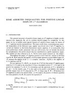
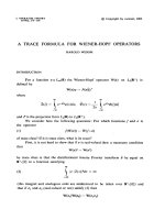
more than one way by ordering its ribbons differently. Here is a example of a placement
of five 4-ribbons below the path corresponding to w = 0010110000010000:
00
1
0
1
1
00000
1
0000
Rather than just counting the total number of placements possible, we refine the count-
ing by keeping track independently of two “statistics” for each placement: the first is the
number n of r-ribbons placed, and the second is their “total height” t,namelythenum-
ber of vertical adjacencies between squares of a same ribbon. In the example displayed

one has n =5,andt = 2 + 2 + 3 + 1 + 0 = 8, where the sum shows the contributions
of the individual ribbons, in order of placement. By contributing a monomial X
n
Y
t
for each placement, and taking the sum over all placements of collections of r-ribbons
below the path corresponding to w, one obtains a two-variable generating polynomial
R
1,1
(w, r) ∈ Z[X, Y ] (the two indices ‘1’ are there to indicate that we have extended w
by bits 1 at both ends). While we do not know any more direct way of describing these
polynomials, we do remark the following property.
1.1.1. Claim. If w is the word obtained by reversing the bits of w,thenR
1,1
(w, r)=
R
1,1
( w, r).
the electronic journal of combinatorics 12 (2005), #R10 3
1.1 Some enumerative problems
Although the polynomials R
1,1
(w, r) are rather laborious to compute by hand,
their computation can be quite easily programmed. The basic observation is that after
having prefixed w by r bits 1 (more are not necessary), each possible placement of a
first r-ribbon is characterised by the simultaneous occurrence of a bit 1 and a bit 0
exactly r places to its right, and that the modification of the path due to placing the
ribbon corresponds to changing those two bits and nothing else. The possibilities of
adding further ribbons can be computed recursively if one takes care to ensure that
they can only be placed further to the right. This can be achieved by removing in the

recursive call the initial part of the word that may no longer be altered, i.e., the part
up to and including the first bit that changed (from 1 to 0; since the bit disappears
anyway there is no need to actually perform this change). To illustrate the simplicity of
the algorithm, we present the complete code in the language of the MuPAD computer
algebra system. We hope that this is readable even to those not familiar with MuPAD;
comments are given after the symbol “//”. The only technical point is the procedure
R11 which prefixes r bits 1 to the word before entering the recursion, and makes sure
the result is expanded and presented as a polynomial in Z[Y ][X].
R := proc(w, r)//w is a list [w
1
, ,w
l
] with w
i
∈{0, 1}
local l, result, i, j , ww;
begin l := nops(w ); result := 1 // count the solution with no ribbons
; for i from 1 to l − r // when l ≤ r, the loop is skipped
do if w[i]=1and w[i + r]=0
then ww := [op(w , i +1 l)] // copy the sub-list [w
i+1
, ,w
l
]
; ww[r ] := 1 // change the bit that was copied from w
i+r
; result := result + R(ww, r ) ∗ X ∗ Y ↑ plus(ww [j ] $ j =1 r − 1)
// the exponent of Y is

r−1

j=1
ww
j
=

i+r−1
j=i+1
w
j
end if
end
for
; result // return the polynomial computed
end
proc;
R11 := proc(w , r) begin poly (poly (R([1 $ r, op(w)], r), [X , Y ]), [X ]) end
proc;
Thus one may compute for w =[0, 0, 1, 0, 1, 1, 0, 0, 0, 0, 0, 1, 0, 0, 0, 0] that R
1,1
(w, 4)
equals
the electronic journal of combinatorics 12 (2005), #R10 4
1.1 Some enumerative problems
1
+X(2 + 2Y +2Y
2
+ Y
3
)
+X

2
(1 + 4Y +7Y
2
+5Y
3
+5Y
4
+2Y
5
+ Y
6
)
+X
3
(Y +6Y
2
+10Y
3
+15Y
4
+12Y
5
+8Y
6
+5Y
7
+2Y
8
+ Y
9

)
+X
4
(2Y
3
+11Y
4
+19Y
5
+23Y
6
+20Y
7
+16Y
8
+8Y
9
+5Y
10
+2Y
11
+ Y
12
)
+X
5
(Y
5
+10Y
6

+21Y
7
+32Y
8
+29Y
9
+24Y
10
+16Y
11
+8Y
12
+5Y
13
+2Y
14
+ Y
15
)
+X
6
(3Y
8
+12Y
9
+28Y
10
+34Y
11
+33Y

12
+24Y
13
+16Y
14
+8Y
15
+5Y
16
+2Y
17
+Y
18
)
+X
7
(Y
11
+10Y
12
+21Y
13
+32Y
14
+29Y
15
+24Y
16
+16Y
17

+8Y
18
+5Y
19
+2Y
20
+Y
21
)
+X
8
(2Y
15
+11Y
16
+19Y
17
+23Y
18
+20Y
19
+16Y
20
+8Y
21
+5Y
22
+2Y
23
+ Y

24
)
+X
9
(Y
19
+6Y
20
+10Y
21
+15Y
22
+12Y
23
+8Y
24
+5Y
25
+2Y
26
+ Y
27
)
+X
10
(Y
24
+4Y
25
+7Y

26
+5Y
27
+5Y
28
+2Y
29
+ Y
30
)
+X
11
(2Y
30
+2Y
31
+2Y
32
+ Y
33
)
+X
12
Y
36
,
and so does R
1,1
( w, 4), where w =[0, 0, 0, 0, 1, 0, 0, 0, 0, 0, 1, 1, 0, 1, 0, 0].
Our claim above can be interpreted in a geometric fashion. If a placement of

r-ribbons below the path corresponding to w is rotated a half turn, one obtains a
placement of r-ribbons above the path corresponding to w according to similar rules
as for the placement below (but note that the order of placement is now from right to
left). So the claim can be reformulated as: for any path that is ultimately vertical at
both ends, and any specified number of ribbons and total height, there are as many
placements possible above the path as there are below the path. Even more than the
original formulation this form begs for a bijective proof, a simple rule to move ribbons
to the other side of the path, so as to define an invertible map from placements of
ribbons on one side to those on the other, preserving the number of ribbons and the
total height; one would expect the inverse map to be given by the same rule after
rotating the configuration a half turn. Yet we have not been able to find such a rule.
Our proof of the claim (given at the end of the paper) will be based on a bijection,
but one corresponding an identity obtained by multiplying both polynomials by an
identical power series. Although a general method exists to deduce from this a bijection
corresponding directly to the claim, the result it is way too complicated to qualify as a
bijective proof.
This negative finding notwithstanding, there are quite a few observations we can
make about this problem that do involve simple bijective constructions. For instance,
when seeing polynomials R
1,1
(w, r) such as the one displayed above, it is hard to miss
a symmetry in the coefficients (although we admit having done so for quite some time):
for every i, the polynomial in Y that is the coefficient of X
12−i
equals the coefficient
of X
i
multiplied by Y
36−6i
. In the general case the coefficient of X

k−i
equals that of
X
i
multiplied by Y
(r−1)(k−2i)
,wherek is the number of bits 0 in w. This suggests that
each placement of ir-ribbons should correspond to a placement of k − i such ribbons
with the same total width (i.e., the number of horizontal adjacencies of squares within
the electronic journal of combinatorics 12 (2005), #R10 5
1.1 Some enumerative problems
a same ribbon). Indeed it does, but the latter will be a placement of ribbons above the
path of w, making the observation about the symmetry of the coefficients equivalent
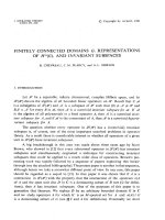
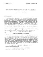
to our claim 1.1.1. To describe the correspondence, first observe that a placement of
r-ribbons is completely determined by it top left and bottom right borders, i.e., by the
path corresponding to w and that path as modified by the placement of all ribbons.
Then if one shifts up the latter path by r units, it will be the top left border of a
unique placement of r-ribbons above the path of w. For instance, here is the placement
obtained from the one displayed earlier (both have total width 7):
00
1
0
1
1
00000
1
0000
Providing the details to prove that this correspondence is well defined and has the
required properties is an instructive exercise that we encourage the reader to solve;
those who would like a hint can turn to lemma 5.2.2 below, which provides a closely

related result.
We can also give bijections proving several sub-cases of our claim 1.1.1. To begin
with, the case r = 1 does not pose much difficulty. Now 1-ribbons are just single squares,
and the total height, being zero always, plays no role. The placement rule forces squares
to be added from left to right below the path of w, advancing at least one column at
each step, so that no column can receive more than one square. Conversely any path
that remains weakly below that of w and weakly above the same path shifted one unit
down (thus leaving room for at most one square in each column) can be obtained for
an appropriate placement of squares; the set of squares of such a placement is known
as a horizontal strip. Each horizontal component of the path of w (a maximal portion
without vertical steps) can be treated in isolation, and can be used to place any number
of squares from 0 up to and including its length, in a unique way; this is true both for
placement above and below it. So one can bring the horizontal strips above and below
the path into bijective correspondence, by requiring that for the former has as many
squares directly above any horizontal component as the latter has directly below it, in
other words that the former has as many squares in any given row as the latter has in
the next row. There is an equivalent algorithmic description that treats the squares one
at a time: traversing the squares of the horizontal strip above the path of w from left
to right, each square is moved one place down, thus crossing the path of w, and then if
necessary slid to the left until it finds a place where it can stay, namely where its left
edge is part of the path of w as possibly modified by the previous placement of squares
below it.
This case can be extended to cover a small part of the claim for general r,namely
the part concerning the leading terms (in Y ) of the coefficients of the X
i
, in other words
the placements where all r-ribbons are completely vertical. For such placements only
the electronic journal of combinatorics 12 (2005), #R10 6
1.1 Some enumerative problems
vertical portions of the path of length at least r effectively produce separate compart-

ments where the ribbons can be placed independently; shorter vertical portions within
such a compartment have no effect on the number of vertical ribbons that can be placed
in it. So again each compartment can accommodate any number of vertical ribbons
from 0 up to and including its width, and does so both above and below. This corre-
spondence too can be described by processing the ribbons above the path from left to
right: each one is moved down across the path, and then to the bottom left up to the
first place where it will fit. Incidentally a similar procedure also works when there are
only horizontal ribbons, but these cases are even more marginal than those involving
only vertical ribbons, since generally only relatively few purely horizontal r-ribbons can
be placed at all.
All this only scratches the surface of the general problem. It should be noted that
one cannot expect a correspondence for the general case where each ribbon above the
path gives rise to a ribbon of the same height below the path, for the simple reason that
the distributions of heights within the collections of placements that should match are
not always the same. This can be seen for the example given (for the given w,there
are 5 different placements of five ribbons that, like the one displayed, produce a total
height 8 as sum of the multiset {{0, 1, 2, 2, 3}}, whereas there are only 4 such placements
for w), but a smaller example is more convincing: below the path of 01000 one can place
a vertical 3-ribbon and a horizontal one (i.e., 3-ribbons of heights 2 and 0, respectively),
but such a pair of 3-ribbons cannot be placed above the same path. This means that it
is important that we count only by total height, and that any correspondence one would
hope to find must have some mechanism for the exchange of height between ribbons (or
alternatively it might treat placements of ribbons as a whole without even considering
individual ribbons, as our first bijection did).
There are two more bijective correspondences that are worth mentioning in this
context, as they provide interesting new points of view, even though they do not tackle
the difficulties just indicated. The first proves the specialisation for Y := 1 of our
claim, i.e., it treats all configurations but ignores the heights of the ribbons. The
second handles the equality of the coefficients of X
1

, i.e., it treats configurations con-
sisting of a single ribbon. If one ignores heights, matters become simpler if one forgets
the geometric description, and views placement of ribbons simply as operations on bit
strings. As we saw, the question of whether an r-ribbon can be placed, and the ef-
fect of placing it, can both be expressed in terms of just one pair of bits, at indices
i and i + r. So placement of different r-ribbons becomes completely independent un-
less the indices i, i

of the bits involved are congruent modulo r (in the latter case we
shall say the ribbons are in the same position class). Thus the possibilities for plac-
ing r-ribbons decompose completely following the r different position classes, and the
specialisation for Y := 1 of R
1,1
(w, r) decomposes as a product

r−1
i=0
R
1,1
(w
(i)
, 1) of
polynomials in X,wherew
(i)
is the word extracted from w, of its bits at indices congru-
ent to i modulo r. So for instance for our example, the specialisation 1 + 7X +25X
2
+
60X
3

+ 107X
4
+ 149X
5
+ 166X
6
+ 149X
7
+ 107X
8
+60X
9
+25X
10
+7X
11
+ X
12
factors as R
1,1
(0100, 1)R
1,1
(0100, 1)R
1,1
(1000, 1)R
1,1
(0010, 1) = (1 +2X +2X
2
+ X
3

) ×
(1 + 2X +2X
2
+ X
3
)(1 + X + X
2
+ X
3
)(1 + 2X +2X
2
+ X
3
). Thus we are back at
the electronic journal of combinatorics 12 (2005), #R10 7
1.1 Some enumerative problems
the case r = 1 we know how to handle. We find the following procedure to transform a
placement of r-ribbons above the path of w into one below, defined by the final value of
a modified copy w

of w. Process the ribbons of any position class from left to right; the
relative ordering between members of different classes is irrelevant. For a ribbon with
initial bit w
i
= 0, search in the current value of w

(which still has w

i
= 0), testing the

bits w

i−r
,w

i−2r
,w

i−3r
, until finding the first bit w

i−kr
= 1; one has w

i−kr+r
=0,
and the bit string w

is modified by setting w

i−kr
:= 0 and w

i−kr+r
:= 1. The mod-
ifications to w

do not always occur in the right order to describe the ribbons of the
placement eventually found, so the independence of operations on different position
classes of ribbons is crucial for proving that the same procedure rotated a half turn

defines an inverse.
We have seen that preserving heights of individual ribbons is not possible in general,
but that ignoring heights altogether makes our problem trivial. The following bijection
for the case of single ribbons gives some insight in the role played by height, without
the complications of interaction between ribbons; it is based on observations in [ShW2].
When an r-ribbon of height h can be placed below the path of w with initial bit w
i
=
1, this means that w
i+r
=0and

i+r−1
j=i+1
w
j
= h, which can also be formulated as

i+r−1
j=i
w
j
= h +1 and

i+r
j=i+1
w
j
= h. Thus the places where a ribbon of height h
can be placed below the path of w correspond exactly to the places where the sum of

r consecutive bits drops from h +1 to h, and similarly a ribbon of height h can be
placed above the path precisely in the places where the value of such sums rises from h
to h + 1. Therefore, starting from a place where such a ribbon can be placed below, one
can always find a place further to the top right where a similar ribbon can be placed
above (since the path ultimately becomes vertical), and from the first such place, the
point of departure can be found back as the first place to its bottom left that will
accommodate an r-ribbon of height h below the path. This establishes our bijection
for the case of single ribbons. One may visualise all possibilities to place r-ribbons of
height h, both below and above, as the points of crossing between the path of w and an
appropriately shifted copy of the same path; see the illustrations after corollary 4.5.2
below.
We close our discussion of this problem with an indication of why we think it has
no simple bijective solution (although we would love to be proved wrong). When one
tries to extend the height preserving procedure for single ribbons to multiple ribbons,
the main difficulty is not so much the exchange of heights that may be necessary, as
the fact that the left to right order among ribbons cannot be preserved. We believe
we could describe a bijection for the case of two ribbons, but it already gets horribly
complicated: when the second ribbon placed needs to move beyond the place where the
first landed, exchange of height must be taken into account, and it may be necessary
to relocate the first ribbon. But the hardest part is to show that one gets a bijection:
the original ribbons must be reconstructed from the pair produced without knowing in
which order those were placed, so there is no question of a step-by-step inverse; a proof
would involve piecing together all the scenarios that can arise. Unless there is some
easy way to read off the order in which ribbons have been placed, it is hard to envisage
a similar technique handling the case of three or more ribbons.
the electronic journal of combinatorics 12 (2005), #R10 8
1.1 Some enumerative problems
If we have spent much time on a problem for which we know no solution, it is
because it is superficially simpler than a second problem, a variant of the first, but one
for which we do have a solution; indeed the solution is closely related to the main result

of this paper (and it will not be detailed in this introduction). The variant is simply
obtained by extending the path described by the finite bit string w not vertically, but
horizontally at both ends; in other words that string is now considered to float in a
sea of bits 0. The conditions for placing collections of r-ribbons remain exactly the
same, as are the two statistics on placements of ribbons (number of ribbons n and total
height t); analogously to the definition of R
1,1
(w, r), the sum of X
n
Y
t
over all possible
placements below this differently extended path will now be denoted by R
0,0
(w, r). One
still has symmetry between placements of ribbons above and below the path.
1.1.2. Claim. If w is the word obtained by reversing the bits of w,thenR
0,0
(w, r)=
R
0,0
( w, r).
If, in keeping with the laws of gravity, we think primarily of placing ribbons above
the path, then the path in our first ribbon placement problem resembles a ledge in an
otherwise sheer rock-face, while the second problem more resembles a Dutch landscape
with a polder to the left, a dike described by the string w, and the sea to the right
(the sea being as high as the dike is not quite realistic, fortunately). We shall therefore
refer to first ribbon placement problem as the alpine problem, and to this second ribbon
placement problem as its polder variant.
The change of landscape modifies the character of our problem in several ways.

While ribbons can lean against the rock face, the sea and the space above sea level
are inaccessible (the top-rightmost vertical edge of each ribbon must belong either to
the dike or to another ribbon). On the other hand, the requirement that the bottom-
leftmost horizontal edge of each ribbon lie on the original path does not put a bound
on the number of ribbons, since the polder provides an infinite supply of such edges.
Indeed, provided w has at least one bit 1, arbitrarily many ribbons can be placed above
the path, for instance using only horizontal ribbons in the polder. Hence the identity of
our second claim is one of formal power series rather than of polynomials. Considering X
to be the principal indeterminate, one has in fact R
0,0
(w, r) ∈ Z[Y ][[X]]: the coefficient
of X
n
is a polynomial in Y of degree at most n(r − 1).
One cannot compute a complete power series R
0,0
(w, r), but the recursive proce-
dure R above can be easily adapted to produce an initial part of such power series (in
finite time!), by adding as a parameter a limit to the degree in X of the terms it should
compute. Thus one verifies that for w = 1011000001 (our earlier example without the
now superfluous bits 0 at either end), both R
0,0
(w, 4) and R
0,0
( w, 4) start as
the electronic journal of combinatorics 12 (2005), #R10 9
1.1 Some enumerative problems
1
+X(2 + Y + Y
2

)
+X
2
(2 + 2Y +4Y
2
+ Y
3
+ Y
4
)
+X
3
(2 + 2Y +5Y
2
+4Y
3
+4Y
4
+2Y
5
+ Y
6
)
+X
4
(2 + 2Y +5Y
2
+5Y
3
+7Y

4
+5Y
5
+5Y
6
+2Y
7
+2Y
8
)
+X
5
(2 + 2Y +5Y
2
+5Y
3
+8Y
4
+8Y
5
+8Y
6
+6Y
7
+6Y
8
+3Y
9
+2Y
10

+ Y
11
)
···
Like before, the configurations counted by R
0,0
(w, r)andbyR
0,0
( w, r) can be inter-
preted respectively as placements of ribbons below and above the same path, and one
would like to prove the claim by means of a bijection between such placements, which
preserves the number of ribbons and their total height.
It is interesting to observe how the case r = 1, that of the horizontal strips, has
changed. In terms of horizontal components of the path, we have effectively gained one
such component, with infinite capacity, whether placing squares above or below the path
(in more formal terms: assuming that w neither begins nor ends with a bit 0, one has
R
0,0
(w, 1) = R
1,1
(w, 1)


n∈N
X
n

, which combinatorialists would write as
R
1,1

(w,1)
1−X
).
But the infinite horizontal component is not the same one in both cases, so if one wants
to maintain the bijection based on this decomposition into horizontal components, one
has to decree that, while most squares from the strip above the path descend below
it and then shift to the left, those that were just above polder level “wrap around at
infinity” and come back from the extreme right, just below sea level. There is nothing
against that as a bijection for r = 1, but as point of departure for the general case
it is better to consider a different bijection, one that moves all squares in the same
direction; this must be left-to-right when going from a horizontal strip above the path
to one below. Doing so, squares arrive under a different horizontal component than the
one they belonged to, and since the capacities of those are unrelated, the level at which
squares will be placed cannot be as neatly predictable as before.
Yet there is a simple method for placing the squares, which is essentially to take
the first available place to the right of their original position, taking into account the
other squares. For instance, for a horizontal strip above the path that consists just of
n squares on the lowest possible (polder) level, and just to the left of the first vertical
edge of the path, the corresponding horizontal strip below the path will occupy the first
n columns to the right of that vertical edge, at whatever level is necessary to be just
below the path. This is possible for any n ∈ N because the squares below any horizontal
component of the path can be filled up from left to right, and a horizontal component of
infinite capacity is available at the end to absorb whatever number of squares might not
fit elsewhere. One wants the same description to define the inverse procedure, which
means in this example that the horizontal strip above the path that occupies the n
columns directly to the left of the last vertical edge of the path should correspond to
the strip of n squares to the right of that edge, just below sea level. To obtain that
result, one must declare columns that contain a square of the original horizontal strip to
be unavailable for placing squares, even if doing so could produce a horizontal strip as
the electronic journal of combinatorics 12 (2005), #R10 10

1.1 Some enumerative problems
output. Therefore the rule should be: for each square, taken in order from left to right
of their original position, move it to the first column to its right that contains neither a
square that was already moved nor one that has yet to be moved. One may verify that
a square may indeed be placed in that column, just below the path, and that the same
rule rotated a half turn will bring back each square to its original position.
Apart from this one-square-at-a-time procedure, there is a description of the same
correspondence that treats all squares at the same time. Imagine a bus driving along
the path from left to right, taking the squares with it as passangers. Each horizontal
edge is a bus stop, where either a square enters the bus (from above), or a square
leaves the bus (from below, but never at a stop where a square entered), or finally, in
case the bus is empty and there is no square waiting at the bus stop, the the bus just
drives on. The importance of this alternative description is not so much its cuteness or
greater efficiency, as the fact that it treats the squares without regard to their individual
identities: while for the purpose of showing equivalence with the earlier description, one
may imagine that each square leaving the bus is the one among the current passengers
that has been aboard the longest, this “choice” has no effect on the result, and all that
matters is keeping track of the number of passengers at each moment.
If we consider the other correspondences that were established for the alpine prob-
lem, we see that the one that was introduced in connection with the symmetry in the
coefficients of the polynomial R
1,1
(w, r) has no counterpart in the polder variant, be-
cause the power series R
0,0
(w, r) has no such symmetry; the two other correspondences
however (the one counting placements of ribbons ignoring their heights, and the corre-
spondence for placements of single ribbons) can be adapted to the polder variant without
much difficulty. The first one of these involves the same reduction to the case r =1
as before, which case is modified as just discussed; the resulting correspondence can be

described by transportation of ribbon by means of a bus with r separate compartments,
one for each of the position classes. The second one is adapted by inverting the direction
of search for a ribbon of appropriate height, due to fact that sums of r consecutive bits
now ultimately become 0 in both directions, rather than r.
Unlike for the alpine problem, a bijection handling the general case and preserving
height can be given here; this fact is at the heart of our main result. Details about the
bijection will be given later, but here is a hint for the impatient. The correspondence is
obtained by the passage of an r-deck bus transporting ribbons, but instead of segregation
by class (an idea we could not endorse anyway) the level of entry and exit of ribbons
is related to height. This level is not identical to the height of the ribbon entering or
leaving however (that would force the output to have the same distribution of heights as
the input, which, like for the alpine problem, cannot always be achieved). Rather it is
the height a ribbon at that position would have in a third placement, one that extends
at both sides of the path of w, and occupies the union of the areas occupied but the
input and output placement (even if the latter is still under construction). Moreover,
the bus operates in a stack-like fashion: whenever a ribbon enters or leaves at some
level, all higher levels are empty.
Neither the alpine problem nor its polder variant quite reflect the original problem
that motivated our work. The problem deals with Young diagrams, whose boundary
the electronic journal of combinatorics 12 (2005), #R10 11
1.2 Background
is given by a path that starts vertically and ends horizontally. By extending w to the
left with bits 1 and to the right with bits 0 one obtains such a path, and it can be
used to define a generating series R
1,0
(w, r). For the purpose of counting placements
of ribbons above rather than below such a path one similarly defines R
0,1
( w, r). The
symmetry observed for the other problems does not exist for this case however; indeed

R
1,0
(w, r) is a proper power series, while R
0,1
( w, r) is a polynomial. The simplest case
is obtained for the empty word . Now no ribbons can be placed at all above the
path, so that R
0,1
(, r) = 1. On the other hand, it can be seen that for any given
multiset of heights, there is exactly one way to place ribbons of those heights below
the path, which does so by weakly decreasing order of height. Thus one deduces that
R
1,0
(, r)=

r−1
h=0
1
1−XY
h
, the generating series of multisets on [r]={0, ,r − 1}.
Instead of the equalities expressed in our first two claims, we observe here that the
generating series for placements below the path is always obtained from the generating
polynomial for those above by multiplication by this fixed power series R
1,0
(, r).
1.1.3. Claim. If w is the reverse word of w,thenR
1,0
(w, r)=R
0,1

( w, r)

r−1
h=0
1
1−XY
h
.
In spite of the different nature of the statement, a bijective proof of this final
claim will turn out to be deduced immediately from one for claim 1.1.2: each multiset
contributing to the factor

r−1
h=0
1
1−XY
h
can be interpreted as describing an initial state
of the bus when it arrives (instead of all decks being empty initially), the occurences
of i ∈ [r] occupying deck i. The bus will still leave the scene empty in this case, but
that too changes if the path ends vertically as in the alpine problem; by allowing for a
non-empty bus both at entry to and at exit from the scene, one obtains a bijective proof
not of the identity of claim 1.1.1, but of the identity derived from it by multiplying both
sides by the power series R
1,0
(, r).
1.2. Background.
The basic form of the Schensted algorithm constructs a bijection between permutations
of n and pairs of standard Young tableaux of equal shape and size n. The two tableaux
shall be referred to as the P -symbol and the Q-symbol, and this terminology will be ex-

tended to all generalisations of the algorithm considered. Its first generalisation already
appears in the original paper [Sche]; it operates on arbitrary sequences of n numbers
(with equal entries allowed), and it constructs as P -symbol a semistandard (or column-
strict) tableau with the same multiset of entries as the word, while the Q-symbol remains
a standard tableau. The symmetry that is lost here is restored in a further generali-
sation by Knuth [Knu], which operates on matrices with natural numbers as entries,
and produces pairs of tableaux which are both semistandard, the multiplicities of their
entries being given by the column sums (for the P -symbol) and the row sums (for the
Q-symbol) of the matrix. The basic Robinson-Schensted correspondence is recovered
when all row and column sums are equal to 1 (the case of permutation matrices); the
generalisation given by Schensted corresponds to the case where the row sums are 1 but
columns sums are arbitrary.
While this generalises the correspondence considerably, the algorithm itself changes
only marginally. The case of a matrix with multiple entries in the same row or column, or
the electronic journal of combinatorics 12 (2005), #R10 12
1.2 Background
entries exceeding 1, is handled by operating in the same way the basic algorithm would
for a permutation matrix derived from it by splitting up rows (each following non-zero
entry getting a fresh row below that of the previous one), multiplexing columns similarly,
and replacing entries m>1bym×m identity sub-matrices. The Schur function s
λ
is the
generating series of the semistandard tableaux of shape λ, so Knuth’s correspondence
provides a bijective proof of the Cauchy identity

i,j
1
1−X
i
Y

j
=

λ
s
λ
(X)s
λ
(Y ). Knuth
also defines a second correspondence that provides a bijective proof of a “dual” identity

i,j
(1 + X
i
Y
j
)=

λ
s
λ
(X)s
λ
t
(Y ). The truncation that has occurred here of the
factors of the left hand side to their terms of degree ≤ 1, means that matrix entries are
now restricted to the values {0, 1}; the transposition of λ in the second factor on the
right means either that P -andQ-symbols have transpose shapes, or (since we prefer
pairs of equal shape) that one is semistandard and the other transpose-semistandard
(row-strict). Like the first one, this second correspondence can be constructed by first

transforming the given matrix to a permutation matrix and then applying the Schensted
algorithm; the only difference is that columns are multiplexed in the opposite sense: each
next non-zero entry gets a fresh column to the left of the previous ones. In the first
correspondence the P-andQ-symbols have symmetric roles, and transposition of the
matrix leads to exchanging them. The second correspondence lacks such a symmetry,
and we shall refer to it as Knuth’s asymmetric correspondence; when not explicitly
calling a correspondence asymmetric, it will be assumed to be a symmetric one.
Fomin has shown in a series of papers [Fom1]–[Fom5] that by identifying the vari-
ous tableaux with paths in a graded partially ordered set or in a directed graph, these
correspondences and many other ones can be described in a general framework that
links local correspondences in the poset or graph to global correspondences involving
pairs of paths. This also means that new correspondences can automatically be defined
as soon as a poset or graph with the required local structure is found. As a conse-
quence of the generality of these constructions, the terms “Schensted correspondence”
and “Knuth correspondence” now acquire a generic meaning, and the specific correspon-
dences mentioned above will referred to as the Robinson-Schensted correspondence and
the RSK correspondence (use this term only for the symmetric one). Our construction
will be an instance of this general framework, so we shall recall the necessary parts
of Fomin’s work in detail in section 2; here we just sketch the outlines. Although the
nature of the poset elements (or vertices of the graph) is not specified, we shall refer
to them as “shapes”; they are Young diagrams in the cases of the Robinson-Schensted
and RSK correspondences.
The general constructions build a two-dimensional array of shapes, from which the
P -symbol and Q-symbol can be read off in the two different directions. To have an
analogue of the Robinson-Schensted correspondence one needs a graded poset whose
connected components are “r-differential”. The most important requirement for this is
that for all shapes µ the number of shapes covering µ exceeds the number of shapes
covered by µ by a fixed number r>0 (the precise requirement is that the commutator
of the “up” and “down” operators for the poset be r times the identity operator). The
Young lattice Y, consisting of Young diagrams ordered by inclusion, is well known to

be 1-differential. The r-differential property can be “made bijective” by means of an
the electronic journal of combinatorics 12 (2005), #R10 13
1.2 Background
r-correspondence, which defines for every shape µ a bijection between on one side the set
of shapes covering µ, and on the other side the union of the set of shapes covered by µ
and a set of r extra values. Given such an r-correspondence, Fomin’s construction will
produce a “Schensted correspondence” between r-coloured permutations of n (where
each term has an additional attribute with r possible values, whence their number
is n!r
n
) and pairs of saturated increasing paths of length n in the poset with a fixed
minimal element as starting point and a common (but varying) end point. For the
Young lattice such paths correspond to standard Young tableaux. For that case there
are two natural choices for a 1-correspondence, one of which leads to the usual Schensted
correspondence by row insertion, the other to its transposed variant (using column
insertion).
For “Knuth correspondences” the general scheme, which is described in [Fom5], is
more complicated. The graded set of shapes used has more than a poset structure: it
is equipped with a directed graph, where edges may relate shapes any number of levels
apart. The entries of the matrices that form the input of the construction come from
a graded but otherwise unstructured set S. For the Young lattice there is edge from
µ to λ whenever µ/λ is a horizontal strip (so that paths correspond to semistandard
tableaux), while S = N. The notion that replaces that of an r-correspondence is what
we shall call a shape datum; it gives for every pair (µ, ν) of shapes a bijection from
shapes κ with edges toward both µ and ν, to pairs (a, λ), where λ is a shape with edges
from both µ and ν,anda ∈ S. It must satisfy a compatibility with the gradings. This
implies that when restricted to edges between shapes at most one level apart, it reduces
to an r-correspondence, where r is the size of the rank 1 subset of S.
The shape datum that matches Knuth’s original construction can be found by
considering how that construction deals with a single matrix entry and one horizontal

stripeachoftheP and Q symbols. Since such a strip is treated just like a skew standard
tableaux corresponding to it (by way of “standardisation”), the mentioned shape datum
is defined by a localised case of the original Schensted correspondence. Shape data in
general however need not be derived from any Schensted correspondence.
The lattice Y
r
is an example of an r-differential poset with r>1, and an
r-correspondence for Y
r
can be defined by fixing 1-correspondences on each of its r fac-
tors. Similarly a graph on Y
r
, and a shape datum for it with graded set S = N
r
,
can be derived in a component-wise fashion from the graph on Y defined by horizontal
strips. These structures lead to Schensted- and Knuth correspondences that factor into
r independent copies of the original ones, which is not very interesting. Another ex-
ampleisgivenbyther-rim hook lattices, whose elements are (single) Young diagrams,
but whose covering relation, adding an r-ribbon, relates shapes that are r levels apart
in Y; the construction of [StWh] provides a Schensted correspondence this example.
However, these lattices are isomorphic to Y
r
by means of the so-called r-quotient map,
and the Stanton-White correspondence thus reduces to the example above.
Yet rim hook lattices can also give rise to Schensted correspondences that do not
decompose into independent ones, by choosing an r-correspondence not derived from
the r-quotient map. Indeed, in [ShW2] a more interesting r-correspondence for the
r-rim hook lattices is defined, which unlike the previous one takes the shapes of the
the electronic journal of combinatorics 12 (2005), #R10 14

1.3 Organisation
ribbons into account. To edges in an r-rim hook lattice one may assign a value h ∈
{0, ,r − 1}, namely the height of the associated r-ribbon; with the r extra values
occurring in an r-correspondence also labelled with that set of values, Shimozono and
White define an r-correspondence preserving these heights. As a consequence, the
Schensted correspondence obtained respects the “spin” statistic on standard r-ribbon
tableaux that gives half the sum of the heights of the ribbons: the sum of the colours
of the input permutation determines the sum of the spins of the output tableaux.
In this paper we define a height respecting shape datum for r-rim hook lattices
equipped with the graphs defined by the notion of horizontal r-ribbon strip (which is
essentially a placement of ribbons of the previous subsection; this notion underlies that of
semistandard r-ribbon tableaux), with graded set S = N
r
. The Knuth correspondence
derived from it shares the “colour-to-spin” property of the Schensted correspondence
of [ShW2], for the natural definitions of the respective statistics on matrices and semi-
standard r-ribbon tableaux. Given the way the original Knuth correspondence is derived
from the Robinson-Schensted correspondence, it may seem a straightforward process to
obtain such a shape datum from the r-correspondence of Shimozono and White; in any
case, this is what we thought initially. It is not. In fact we were unable to find a shape
datum that would reduce, when appropriately restricted, to that r-correspondence; this
is essentially for the same reason that we know no bijective proof of our claim 1.1.1.
Instead our shape datum reduces to the transpose r-correspondence (so to speak its
column insertion variant, although that term is not very appropriate in the r-ribbon
case). Since horizontal r-ribbon strips (unlike r-ribbons) lack transposition symmetry,
this distinction is significant.
Even more surprisingly, our correspondence does not reduce for r = 1 to the shape
datum corresponding to the RSK correspondence, but to one associated to the so-
called Burge correspondence. These shape data are fundamentally different, even if
the RSK correspondence and the Burge correspondence are related (the relation also

involves the Sch¨utzenberger involution on semistandard tableaux). The most crucial
observation we had to make in order to find the shape datum used in our construction,
was that although the shape datum for the Burge correspondence can be defined by
iterating Schensted column-insertion, it has an alternative single-pass description (much
like the bus transport in the previous subsection) that can easily be adapted to the
context of semistandard r-ribbon tableaux.
1.3. Organisation.
The remainder of this paper is organised as follows. In section 2 we recall in detail
Fomin’s general framework to define Schensted and Knuth correspondences. In sec-
tion 3 we describe the shape data for the RSK correspondence, and for the Burge
correspondence, while also indicating how the global correspondences defined by them
are related. We close that section by giving the most trivial examples of correspondences
with r>1, namely those using Y
r
. In section 4 we recall the definitions involving r-rim
hook lattices and semistandard r-ribbon tableaux, and the factoring of many questions
concerning r-ribbons due to the r-quotient map; we then discuss the spin statistic and
the r-correspondence defined by Shimozono and White, which do not factor in this way.
the electronic journal of combinatorics 12 (2005), #R10 15
1.4 Acknowledgement
In section 5 we present our main result, the shape datum that leads to a spin preserv-
ing Knuth correspondence from matrices with entries in N
r
to pairs of semistandard
r-ribbon tableaux. In section 6 we similarly generalise Knuth’s asymmetric correspon-
dence to one from matrices with entries in {0, 1}
r
to pairs consisting of a semistandard
and a transpose semistandard r-ribbon tableau.
Although the presentation of our new constructions is our central goal around which

the paper is organised, much of it can also be considered as an expository one of the
various constructions on which we build forth. For this reason our pace will often be
leisurely and our discussion informal. We have tried to limit the formal definitions and
notations used, and most of those that are introduced serve a very localised purpose;
giving them will therefore be postponed to the moment they are actually used. We
shall also take time to discuss some matters that are not essential to our constructions,
notably the reasons why certain approaches we tried were not successful.
1.4. Acknowledgement.
The author would like to thank Thomas Lam for a number of critical comments that
helped improve this paper.
§2. Review of Fomin’s constructions.
2.1. Schensted correspondences.
Let us recall the framework described in [Fom3]–[Fom4] for defining Schensted corre-
spondences, while simplifying it slightly by omitting some generality that is not needed
in the current paper. For a treatment of just the case of the Robinson-Schensted corre-
spondence, we may refer to [vLee1, §3]. We keep in mind that special case throughout
the discussion, and keep our notation close to what is customary there.
One starts with graded set P of shapes, whose rank function P→N is written
λ →|λ| andissuchthateachsetP
i
= { λ ∈P||λ| = i } is finite. A structure of graded
graph on P is defined by giving a relation contained in

i∈N
P
i
×P
i+1
,inotherwordsa
set of edges (λ, µ) with |µ| = |λ| + 1. Although two different structures of graded graph

on the same set P are used in the theory (one for each of the “up” and “down” operators
introduced below), these always coincide in the cases we shall consider, so we use a single
symbol ‘≺’ to denote this relation. Its reflexive and transitive closure will be denoted
by ‘≤’, which makes P into a graded poset, from which one can retrieve the graded
graph as its Hasse diagram. The latter need not be connected, and we shall encounter
examples where this is not the case; however, since we shall be mainly interested in
paths in the graph, we lose no generality by considering one connected component at
the time. For λ ≤ µ we define a path of shape µ/λ to be a monotonously rising path
λ = λ
0
≺ λ
1
≺ ··· ≺ λ
n
= µ in the graph, and we shall write |µ/λ| = n = |µ|−|λ|.
Due to further requirements each connected component of the graph will have a unique
minimal element, which by a shift in the grading on that component could be assumed
to have rank 0. A path of shape µ/λ where λ is the minimal element of its component
will be called simply a path of shape µ.
the electronic journal of combinatorics 12 (2005), #R10 16
2.1 Schensted correspondences
Let ZP denote the free Z-module on the set P of shapes; one defines endomorphisms
U, D of ZP by their action on basis elements: U: λ →

µλ
µ and D: λ →

µ≺λ
µ
(these are well defined by the finiteness of each P

i
). The basic assumption we make of
our graded graph is the commutation relation
D ◦ U = U ◦ D + r1 (1)
for some r ∈ N
>0
,where1 is the identity operator. It is clear that in any case both mem-
bers of this equation preserve the grading. So if one applies the equation to some λ ∈P
i
,
it states two things: taking the coefficient of λ itself, one gets
#{ µ ∈P
i+1
| µ  λ } =#{ µ ∈P
i−1
| µ ≺ λ } + r, (2)
and taking the coefficient of some λ

∈P
i
with λ = λ

one gets
#{ µ ∈P
i+1
| µ  λ; µ  λ

} =#{ µ ∈P
i−1
| µ ≺ λ; µ ≺ λ


}. (3)
The latter condition implies that if there is any path between two shapes, then there
is one that is composed of a monotonous descending path followed by a monotonous
rising path, so in particular each connected component of P has a unique minimal
element. Therefore equation (1) means that each such component is an r-differential
poset as defined in [Stan1, definition 1.1]. One also sees easily that if condition (3)
holds for all λ, λ

, then the cardinalities in the equation cannot exceed 1. In case a
component of P is a lattice, that condition amounts to the lattice being modular (i.e.,
|λ ∧ µ| + |λ ∨ µ| = |λ| + |µ|).
The classical example of a 1-differential poset is the Young lattice Y consisting
Young diagrams (finite order ideals of N
2
) ordered by inclusion. A partition λ
0
≥ λ
1
≥
···represents a Young diagram λ = { (i, j) ∈ N
2
| i<λ
j
}, whose elements are referred
to (and displayed) as squares. In Y, a path (0) = λ
0
≺ ··· ≺ λ
n
= λ of shape λ

corresponds to a standard Young tableau of shape λ, which can be displayed by filling
the squares of λ with the numbers in [n]={0, ,n− 1} in such a way that for each i
the set of entries in the diagram λ
i
is [i]. Thus the standard Young tableau displayed
as
0 2 3 5
1 6
4
corresponds to the path
◦≺
≺ ≺ ≺ ≺ ≺ ≺ .
For our purposes we shall consider standard Young tableaux of shape λ just to be paths
of shape λ.
Let us check that Y is a 1-differential poset. Since Y is a modular (even distribu-
tive) lattice (with λ ∧ µ = λ ∩ µ and λ ∨ µ = λ ∪ µ), it suffices to check condition (2),
which states that for any Young diagram there is one more square that can be added
the electronic journal of combinatorics 12 (2005), #R10 17
2.1 Schensted correspondences
to it than there are squares that can be removed from it. Although this is quite easy
to see, we give a formal argument, since variations of it will be used later to prove
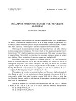
less obvious statements. A Young diagram λ is completely determined by its edge se-
quence δ(λ), a doubly infinite bit string describing (as in §1.1) the segments of the path
that forms the edge of λ, from bottom left to top right (for a formal definition of δ(λ)
see [vLee2]; it is essentially the (Com´et) code C
λ
of λ used in [Stan2, Exercise 7.59],
but with all bits complemented). The bits eventually become 1 to the left (for the
rows of length 0) and 0 to the right (for the columns of height 0). Occurrences of a
substring “10” correspond to squares that can be added to the diagram, causing the

substring to be replaced by “01”, occurrences of which therefore correspond to squares
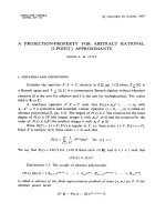
that can be removed. We illustrate this for the diagram λ of (6, 4, 3, 3, 1), and the
bracketed substring of δ(λ)=(···1101001[10]100100 ···).
1
1
0
1
00
1
1
0
1
00
1
00
0
1
In any word over the alphabet {0, 1} the occurrences of “10” and “01” are perfectly
interleaved from left to right. The limiting behaviour of letters in both directions ensures
that the set of these occurrences is finite and non-empty, and that the first and the last
ones are occurrences of “10”. Therefore the number of occurrences of “10” exceeds that
of occurrences of “01” by one.
As is shown in [Stan1], many enumerative properties can be derived uniformly for
all r-differential posets, i.e., they depend only on the identity (1). In [Fom4] bijections
corresponding to such identities are constructed, but this requires some additional ingre-
dients (as could be expected, since otherwise there is nothing to discriminate between
the elements of P), namely a family of bijections that correspond to local instances
of (1), i.e., linking the sets counted by the members of equations (2) and (3). In fact
one needs not bother about (3), since we have observed that those sets are either empty
or singletons, which leaves no choice for a bijection. It is not obvious which set should

be counted by the final term ‘r’in(2);anyr element set disjoint from P would do.
Recall that we denoted by [r]ther element order ideal { i ∈ N | i<r} = {0, ,r− 1}
of N, which we take as our standard r-element set. We could let the mentioned term ‘r’
correspond to [r], but it will be clearer, and more flexible for generalising later, to take
a set e
[r]
= { e
i
| i ∈ [r] } of r symbols that are reserved to serve as exceptional values.
We then define an r-correspondence on P to consist of a family of bijections
b
λ
: { µ ∈P|µ  λ }→{µ ∈P|µ ≺ λ }∪e
[r]
for λ ∈P.(4)
the electronic journal of combinatorics 12 (2005), #R10 18
2.1 Schensted correspondences
(In fact r-correspondences are defined in [Fom4] as bijections between edges rather
than between vertices of the graph, but in the situation we are considering, the simpler
notion above gives the same information). Assuming that (1) holds, an r-correspondence
always exists, although it might be hard to specify; usually however, the proof of (1)
suggests a natural choice of an r-correspondence. For Y, we see that there are in fact
two natural choices: one may either associate to any occurrence of “10” in δ(λ)the
occurrence of “01” to its left, except that the leftmost occurrence of “10” is sent to the
exceptional value e
0
, or one can do the same thing with “left” replaced by “right”. Due
to the symmetry of Y with respect to transposition, there is no fundamental difference
between the two choices, but the choice that will lead to the Schensted correspondence
in its usual form (i.e., using row insertion) is to move to the right: each square that can

be added will then correspond to the square that can be removed from the row directly
above it, with the square that can be added to the topmost row corresponding to e
0
.
Once an r-correspondence has been fixed, it may be used to define bijective corre-
spondences that match identities derived from equation (1). Although there are many
of these, we focus on the following one:
  | D
n
(U
n
())  = n!r
n
for a minimal element  of P,andn ∈ N,(5)
where the scalar product is the canonical one in ZP, so that the left hand side gives the
coefficient of  in D
n
(U
n
()). The identity can be derived by showing that when (1) is
used repeatedly to rewrite D
n
◦U
n
as a sum of terms of the form U
i
◦D
i
with 0 ≤ i ≤ n,
then U

0
◦ D
0
= 1 occurs with coefficient n!r
n
. Since the operators D and U are adjoint
with respect to the scalar product, the left hand side of (5) can also be written as
 U
n
() | U
n
() .Everyλ ∈P
||+n
with  ≤ λ occurs in U
n
(), with as multiplicity
the number of paths of shape λ, so (5) states that the sum of the squares of these
numbers equals n!r
n
.ForP = Y, paths of shape λ are standard tableaux of shape λ,
and for the value r = 1 applicable to this case the number n!r
n
= n! of course counts
the permutations of n, so here equation (5) gives the enumerative identity that the
Robinson-Schensted correspondence proves. Any correspondence similarly proving (5)
for some r-differential poset, with the right hand side n!r
n
counting the r-coloured
permutations of n, can therefore be considered to be a generalisation of the Robinson-
Schensted correspondence.

Given an r-correspondence on P, one can obtain such a correspondence by defining,
for any minimal element  of P and n ∈ N, an intermediate set of “growth diagrams”
that is in bijection both with the set of pairs of paths of some common shape λ ∈P
||+n
with  ≤ λ and with the set of r-coloured permutations of n. These bijections are just
projections that extract partial information from a growth diagram; their bijectivity
therefore means that growth diagrams can always be uniquely reconstructed from such
information. We formally define r-coloured permutations of n to be matrices (A
i,j
)
i,j∈[n]
with entries A
i,j
∈{0}∪e
[r]
such that |A
i,j
|
i,j∈[n]
is a permutation matrix, where we
set |e
i
| =1foralli ∈ [r]. Specifying an r-coloured permutation of n is equivalent to
giving the permutation σ of n such that |A
i,j
| = 1 whenever σ(i)=j,andthen values
A
i,σ(i)
∈ e
[r]

(i ∈ [n]), which explains the name.
the electronic journal of combinatorics 12 (2005), #R10 19
2.1 Schensted correspondences
2.1.1. Definition. Let P be a graded poset equipped with an r-correspondence
{ b
λ
| λ ∈P}as defined by equation (4), and let a minimal element  of P and n ∈ N be
fixed. A growth diagram, or Schensted-growth, relative to these data consists of a pair
of maps, the first one mapping [n +1]
2
→Pand written (k,l) → λ
(k,l)
, the second one
mapping [n]
2
→{0}∪e
[r]
and written (k, l) → A
k,l
, that satisfy the following conditions
for all k, l ∈ [n]:
(0) λ
(0,0)
= ;
(1) λ
(k,l)
 λ
(k,l+1)
and λ
(k,l)

 λ
(k+1,l)
;
(2) λ
(n,l)
≺ λ
(n,l+1)
and λ
(k,n)
≺ λ
(k+1,n)
;
(3) |λ
(k,l)
| = || +

(i,j)∈[k]×[l]
|A
i,j
|;
(4) If λ
(k,l+1)
= λ
(k+1,l)
≺ λ
(k+1,l+1)
then, putting µ = λ
(k,l+1)
, κ = λ
(k+1,l+1)

and
v = b
µ
(κ), one has either λ
(k,l)
= v (if v ∈P), or A
k,l
= v (if v ∈ e
[r]
).
The alternative term “Schensted-growth” for growth diagram will be used later to
distinguish this notion from a similar one used in relation to Knuth correspondences.
It follows from (2) and (3) that (A
i,j
)
i,j∈[n]
is an r-coloured permutation of n.One
also has λ
(i,0)
=  = λ
(0,i)
for i ∈ [n +1], so that P =(λ
(n,0)
≺ λ
(n,1)
≺ ··· ≺ λ
(n,n)
)
and Q =(λ
(0,n)

≺ λ
(1,n)
≺ ···≺ λ
(n,n)
) are paths of shape λ
(n,n)
; this defines the two
mentioned projections. For the permutation σ of n corresponding to |A
i,j
|
i,j∈[n]
,one
has λ
(k,l)
= λ
(k+1,l)
in condition (1) if and only if σ(k) ≥ l,andλ
(k,l)
= λ
(k,l+1)
if and
only if σ
−1
(l) ≥ k. In particular |A
k,l
| = 1 implies that λ
(k,l)
= λ
(k+1,l)
= λ

(k,l+1)
,
so in condition (4) one has A
k,l
= 0 in the case v ∈P(since b
µ
(κ) = µ), while
λ
(k,l)
= λ
(k+1,l)
= λ
(k,l+1)
in the case v ∈ e
[r]
.
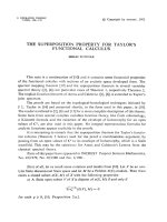
It is convenient to display a growth diagram by attaching the shape λ
(k,l)
to the
point (k, l) of a grid (with k increasing downwards and l increasing to the right), and
writing the matrix entry A
k,l
into the square of that grid with corners (k, l), (k, l +1),
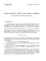
(k +1,l), and (k +1,l+ 1). Figure 1 thus illustrates a growth diagram for P = Y
with the mentioned left-to-right 1-correspondence; non-zero matrix entries, which due
to r = 1 are necessarily equal to e
0
,areindicatedby‘’.
The pair (P, Q) gives the values of λ
(i,j)

for (i, j) ∈ [n +1]
2
\ [n]
2
, so reconstruction
of a growth diagram by decreasing values of k and l, from arbitrary (P,Q), will be
possible if for any k, l ∈ [n] one can uniquely determine the shape λ = λ
(k,l)
and the
matrix entry A
k,l
once the shapes µ = λ
(k,l+1)
, ν = λ
(k+1,l)
,andκ = λ
(k+1,l+1)
are
known. And indeed this is the case: if κ is equal to µ or to ν,thenλ
(k,l)
will be
equal to the other, and otherwise if µ and ν are distinct, then λ
(k,l)
will be the unique
element covered by both (which exists because both are covered by κ); in both these
cases A
k,l
= 0. The remaining case µ = ν = κ is the one handled by condition (4);
there, as we saw, both λ and A
k,l

are always determined. From this description one
sees that the differential version |κ|−|µ|−|ν| + |λ| = |A
k,l
| of condition (3) holds in all
cases; the verification of the remaining requirements is now easy. A growth diagram can
be similarly reconstructed from the matrix (A
i,j
)
i,j∈[n]
, by increasing values of k and l:
one determines λ
(k+1,l+1)
once λ
(k,l)
, λ
(k,l+1)
, λ
(k+1,l)
(and of course A
k,l
)areknown;
to prove this, similar cases as above can be distinguished, with the case |A
k,l
| =1being
singled out first.
the electronic journal of combinatorics 12 (2005), #R10 20
2.1 Schensted correspondences
0123 45678
0
◦◦◦◦◦◦◦◦◦

1
◦◦◦◦ ◦

2
◦◦

3
◦◦

4
◦

5
◦

6
◦

7
◦

8
◦

Figure 1. Schensted-growth for Y with σ =

01234567
41602753

, P =

0 2 3
1 5 7
4 6
,andQ =
0 2 5
1 4 6
3 7
.
For P = Y with the chosen 1-correspondence, the resulting bijection between
permutations and pairs of standard Young tableaux is the classical Robinson-Schensted
correspondence. The Schensted insertion of the permutation entry σ(i) corresponds to
the computation, given the line λ
(i,0)
 ···  λ
(i,n)
of the growth diagram and the
entry A
i,σ(i)
= e
0
, of the next line λ
(i+1,0)
···λ
(i+1,n)
.
The method of reconstructing a growth diagram from (P, Q)orfrom(A
i,j
)
i,j∈[n]
can be viewed as a data-flow network consisting of n

2
copies of the r-correspondence
respectively of its inverse: for every pair k, l ∈ [n], a copy of the r-correspondence links
the values A
k,l
, λ
(k,l)
, λ
(k+1,l)
, λ
(k,l+1)
,andλ
(k+1,l+1)
. In fact we had to complement
the r-correspondence with several cases (where no choice was involved) to determine all
necessary values, but in the full generality of [Fom4] these cases are already incorporated
into the r-correspondence itself. Moreover that r-correspondence operates on the edges
rather than on the vertices of the square λ
(k,l)
, λ
(k+1,l)
, λ
(k,l+1)
,andλ
(k+1,l+1)
, with
each of the two output edges being one of the inputs to a unique other copy of the
r-correspondence (unless it is part of the final output), so that the data-flow nature is
even more clearly visible there.
One may observe that apart from extraction of the pair (P, Q)ofpathsinP,or

of A,ther-coloured permutation of n, other projections allow unique reconstruction of
a growth diagram as well: it suffices to know λ
(i,j)
for all (i, j) on some lattice path
from (n, 0) to (0,n), and all matrix entries A
i,j
that lie below and to the right of that
path. Starting with the shapes along the bottom and right edges of the diagram as
given by (P, Q), one can therefore replace this information by the shapes along paths
that are gradually modified to eventually become the path along the left at top edges,
the electronic journal of combinatorics 12 (2005), #R10 21
2.2 Knuth correspondences
while retaining all matrix entries that the path has moved across; then at each moment
one has complete information to determine the entire growth diagram. This procedure
may be interpreted as describing the process of rewriting the left hand side of (5) to its
right hand side: it provides a way to trace, and thus obtain a matching between, the
contributions to these two expressions and to all intermediate ones.
2.2. Knuth correspondences.
We shall now consider the generalisation of this construction to “Knuth correspon-
dences”, which is described in [Fom5]. The fundamental difference with Schensted cor-
respondences is that matrix entries will be chosen independently, without the restriction
that they should give rise to a permutation matrix. Matrix entries will be chosen from
some graded set S, whose rank function S → N written x →|x| is such that each set
S
i
= { x ∈ S ||x| = i } is finite, and S
0
= {0}. We shall define growth diagrams similar
to those defined in above, for which in particular condition 2.1.1(4) will be required.
From the independence of matrix entries it then follows that one has to allow arbitrar-

ily large differences of rank between shapes on adjacent grid points (at least, growing
with n), even if all non-zero matrix entries should have rank 1. Therefore one needs to
equip P with a relation that unlike ‘’ can hold between shapes any number of levels
apart. We shall denote this relation, which in general will not be transitive, by ‘’,
with µλmeaning the same as λµ. At this point we make no assumption about
this relation other than that λµand |λ| = |µ| imply λ = µ. When λµwe shall
as before write |µ/λ| = |µ|−|λ|.
The adaptation of the rules governing growth diagrams is quite straightforward.
Each matrix entry a = A
i,j
∈ S is associated to a square of the grid, the corners of
which have shapes attached to them, which as before we shall designate by λ = λ
(i,j)
,
µ = λ
(i,j+1)
, ν = λ
(i+1,j)
,andκ = λ
(i+1,j+1)
; these satisfy λµκand λνκ.
From condition 2.1.1(4) it follows moreover that
|κ|−|ν|−|µ| + |λ| = |a|. (6)
As in the case of Schensted correspondences, we wish that given µ, ν,andκ,theshapeλ
and the entry a can be uniquely determined, and that similarly given λ, µ, ν and a,the
shape κ can be determined. In other words, for every pair µ, ν ∈Pthere should be a bi-
jection between the sets { κ ∈P|κµ; κν} and { (a, λ) ∈ S ×P|λµ; λν}
such that equation (6) holds whenever (a, λ) corresponds to κ. Such a family of bijec-
tions will be a central notion of this paper, so we state a formal definition.
2.2.1. Definition. Let P be a graded set equipped with a relation ‘’, and S a graded

set. A shape datum for (P,,S) consists of a family (b
µ,ν
)
µ,ν∈P
of bijections
b
µ,ν
: { κ ∈P|µκν}→{(a, λ) ∈ S ×P |µλν}, (7)
such that |κ|−|ν|−|µ| + |λ| = |a| holds whenever (a, λ)=b
µ,ν
(κ).
In order for a shape datum to exist, (P,,S) must satisfy an enumerative iden-
tity that is most easily expressed using formal power series. We shall use the ring
the electronic journal of combinatorics 12 (2005), #R10 22
2.2 Knuth correspondences
End(ZP)[[X, Y ]] of formal power series in indeterminates X, Y over the ring of endo-
morphisms of ZP. Such a power series can be applied to an element of ZP to give a
formal sum of monomials in X and Y with coefficients in ZP, i.e., an element of the
Z[[X, Y ]]-module ZP[[X, Y ]]. This action on elements of ZP can be extended with-
out problem to an action on power series, in other words we can interpret elements
of End(ZP)[[X, Y ]] as endomorphisms of ZP[[X, Y ]]. We define two such elements
U
X
,D
Y
∈ End(ZP)[[X, Y ]] in terms of their action, by requiring
U
X
(λ)=


µλ
X
|µ/λ|
µ and D
Y
(λ)=

µλ
Y
|λ/µ|
µ for all λ ∈P.(8)
Let F
S
(T ) ∈ Z[[T ]] be the rank generating series

a∈S
T
|a|
=

i∈N
c
i
T
i
of S,where
c
i
=#S
i

. Then the enumerative requirement for the existence of a shape datum will
be
D
Y
◦ U
X
=(U
X
◦ D
Y
)

F
S
(XY )

. (9)
If one writes U
X
=

i∈N
U
i
X
i
and D
Y
=


i∈N
D
i
Y
i
, then taking the coefficient of
X
i
Y
j
in (9) gives
D
j
◦ U
i
=

k≤min{i,j}
c
k
(U
i−k
◦ D
j−k
). (10)
When both members of this equation are applied to µ, the values obtained are of rank
|µ| + i − j, and if one takes the coefficient of some ν ∈P
|µ|+i−j
, the resulting numbers
count the subsets of the domain and codomain of b

µ,ν
for which | κ| = |µ|+i respectively
|λ| = |µ|−j + |a|; these are subsets that should be in correspondence under b
µ,ν
if it
is to satisfy (6). Taking i = j = 1 in (10) gives D
1
◦ U
1
= U
1
◦ D
1
+ c
1
1,whichshows
that the current situation extends the one considered earlier: if one defines λ ≺ µ when
λµand |λ| +1 =|µ|, then (2) and (3) will hold, with r = c
1
. There is however
no easy way to extend the structure (P, ≺)to(P,,S); indeed it is not obvious why
any combinatorial structures satisfying (9) should exist at all. Yet several examples are
given in [Fom5], among which the example corresponding to the RSK correspondence
(described in the next section), which is the one that will concern us most.
Once one has defined a shape datum, the construction of a global “Knuth” cor-
respondence from it is straightforward, by analogy to the construction of Schensted
correspondences. In fact, matters are slightly simpler since there is no need to explic-
itly distinguish cases according to the differences of rank between shapes associated to
neighbouring points of the grid, as all possible cases are already catered for by the shape
datum itself. Calling  ∈Pminimal when λimplies λ = , we have the following

notion of growth diagram.
2.2.2. Definition. Let (b
µ,ν
)
µ,ν∈P
be a shape datum for (P,,S) as defined in 2.2.1,
and let a minimal element  of P,andn, m ∈ N be fixed. A growth diagram, or
Knuth-growth, relative to these data consists of a pair of maps, the first one mapping
[m +1]×[n +1]→Pand written (k, l) → λ
(k,l)
, the second one mapping [m] ×[n] → S
and written (k, l) → A
k,l
, that satisfy the following conditions, for all k ∈ [m] and
l ∈ [n]:
the electronic journal of combinatorics 12 (2005), #R10 23
2.2 Knuth correspondences
(0) λ
(0,n)
=  = λ
(m,0)
;
(1) λ
(k,l+1)
λ
(k+1,l+1)
,andλ
(k+1,l)
λ
(k+1,l+1)

;
(2) With λ = λ
(k,l)
, µ = λ
(k,l+1)
, ν = λ
(k+1,l)
,andκ = λ
(k+1,l+1)
, one has (A
k,l
,λ)=
b
µ,ν
(κ).
Note that there is no longer a need to require explicitly that |λ
(k,l)
| = || +

(i,j)∈[k]×[l]
|A
i,j
|, as this follows easily from the fact that b
µ,ν
respects equation (6).
We shall again consider two projections from the set of growth diagrams: one ex-
tracting the matrix A =(A
k,l
)
k∈[m],l∈[n]

, the other extracting the pair of paths
P =(λ
(m,0)
λ
(m,1)
 ··· λ
(m,n)
)andQ =(λ
(0,n)
λ
(1,n)
 ··· λ
(m,n)
).
In the latter, P and Q will be called paths of shape λ
(m,n)
(or more explicitly of
shape λ
(m,n)
/)in(P,). Besides this (final) shape, a property of paths describ-
ing the successive ranks of the intermediate shapes is important: we define the weight
of a path p =(λ
0
 ··· λ
n
) to be the vector wt(p)=(|λ
i+1
/λ
i
|)

i∈[n]
. One has
wt(P )=


i∈[m]
|A
i,j
|

j∈[n]
and wt(Q)=


j∈[n]
|A
i,j
|

i∈[m]
, in other words, the
weights of the paths P, Q are the vectors of column sums of ranks and of row sums
of ranks, respectively, of the matrix A. Both projections can be seen to be bijections,
respectively to the set of all matrices with coefficients in S and to the set of all pairs
of paths in (P,) of equal shape, in the same way as for the Schensted-growths. The
correspondence between the matrices A and pairs (P, Q) of paths, defined by composing
one projection with the inverse of the other, is the Knuth correspondence for (P,,S)
associated to the given shape datum.
Like Schensted correspondences, Knuth correspondences imply enumerative iden-
tities, but since the sets linked by any bijection b

µ,ν
are infinite, these follow from the
mentioned matching of the weights of (P, Q)andofA. One uses two sets of indeter-
minates X
[n]
= { X
j
| j ∈ [n] } and Y
[m]
= { Y
i
| i ∈ [m] } to record the weights of P
and Q respectively: the contribution of each pair (P, Q) will be given by the monomial
X
wt(P )
Y
wt(Q)
, where as usual X
(a
0
, ,a
n−1
)
abbreviates X
a
0
0
···X
a
n−1

n−1
.Bywhatwas
observed above, that monomial can also be expressed in terms of the matrix A corre-
sponding to (P,Q)as

i∈[m],j∈[n]
(X
j
Y
i
)
|A
i,j
|
. Summation of that monomial over all
m × n matrices A with entries in S gives

i∈[n],j∈[m]
F
S
(X
i
Y
j
) (note that we disentan-
gle the indices, the mixing of which was caused by the unfortunate but conventional
choice of reading off P from the growth diagram by varying the second index). If one
defines the generating series G
λ
(X

[n]
)=

P
X
wt(P )
, where the sum is over all paths
P =( = λ
0
 ···λ
n
= λ), then one finds the identity

i∈[n],j∈[m]
F
S
(X
i
Y
j
)=

λ∈P
G
λ
(X
[n]
)G
λ
(Y

[m]
) (11)
Noting that G
λ
(X
[n]
)=

λ | U
X
n−1
···U
X
0
()

, this equation can be seen to follow
directly from (9):
the electronic journal of combinatorics 12 (2005), #R10 24
3 Examples of shape data

λ∈P
G
λ
(X
[n]
)G
λ
(Y
[m]

)=

U
Y
m−1
···U
Y
0
() | U
X
n−1
···U
X
0
()

=

 | D
Y
0
···D
Y
m−1
U
X
n−1
···U
X
0

()

=

 | U
X
n−1
···U
X
0
D
Y
0
···D
Y
m−1
()


i∈[n],j∈[m]
F
S
(X
i
Y
j
)
=

i∈[n],j∈[m]

F
S
(X
i
Y
j
),
(12)
where the last step follows from the fact that  is minimal. This derivation demonstrates
(again) the straightforwardness of deriving the global Knuth correspondence from the
shape datum.
§3. Examples of shape data.
3.1. The shape datum for the RSK correspondence.
Let us now consider the RSK correspondence, and its shape datum. In this case S = N,
P = Y, and the relation λµmeans that µ/λ is a horizontal strip: λ ⊆ µ,and
the skew diagram of µ/λ (the set-theoretic difference of diagrams µ \ λ) has at most
one square in any column. When λµ, a specific path in (P, ≺)(suchpathsare
also called skew standard tableaux) of shape µ/λ is defined by requiring that in the
successive diagrams along the path from λ to µ, the squares are added in left to right
order, i.e., by (strictly) increasing column number. By interpolating in this way each
of its horizontal strips (while eliminating any strips of size 0), a path in (P,)canbe
transformed into a (skew) standard tableau of the same shape, called its standardisation.
The RSK correspondence, in the “extraction” direction (determining the matrix A from
apair(P, Q) of equal shaped paths in (P,)), can now be informally described as
follows. First the standardisations of P and Q are determined, and then the Schensted-
growth corresponding to this pair of standard Young tableaux is constructed. Due to
the initial interpolation, this growth diagram is defined on a grid that is too extensive
for the matrix A one wishes to find; therefore the grid is now reduced by forgetting
its points on horizontal or vertical lines that were introduced by the interpolation, so
that the paths remaining along the bottom and right edges are the original P and Q,

before standardisation. The shapes associated to the remaining grid points will be the
ones of a Knuth-growth; the matrix entry to be associated with a grid square whose
corners carry shapes

λµ
νκ

is |κ|−|ν|−|µ|+|λ|, which is the sum over the corresponding
rectangular area of the Schensted-growth of the associated permutation matrix entries.
Proving that this description defines (a Knuth-growth for) a shape datum for (Y,)
essentially amounts to showing that the shapes associated to adjacent grid points after
reduction differ by horizontal strips; this can be deduced easily from a consideration of
local portions of the Schensted-growth consisting of just two horizontally or vertically
adjacent squares of the grid for that growth diagram.
Let us demonstrate the construction by a concrete example, which we take from
Knuth’s original paper [Knu]. The semistandard tableaux can be readily interpreted as
paths, so for instance
the electronic journal of combinatorics 12 (2005), #R10 25