Computational Intelligence in Automotive Applications Episode 1 Part 3 ppt

Visual Monitoring of Driver Inattention 25
(a) Frame 187 (b) Frame 269 (c) Frame 354 (d) Frame 454 (e) Frame 517
(f) (g)
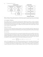
Fig. 5. Tracking results for a sequence
To continuously monitor the driver it is important to track his pupils from frame to frame after locating
the eyes in the initial frames. This can be done efficiently by using two Kalman filters, one for each pupil, in
order to predict pupil positions in the image. We have used a pupil tracker based on [23] but we have tested
it with images obtained from a car moving on a motorway. Kalman filters presented in [23] works reasonably
well under frontal face orientation with open eyes. However, it will fail if the pupils are not bright due to
oblique face orientations, eye closures, or external illumination interferences. Kalman filter also fails when
a sudden head movement occurs because the assumption of smooth head motion has not been fulfilled. To
overcome this limitation we propose a modification consisting on an adaptive search window, which size is
determined automatically, based on pupil position, pupil velocity, and location error. This way, if Kalman
filtering tracking fails in a frame, the search window progressively increases its size. With this modification,
the robustness of the eye tracker is significantly improved, for the eyes can be successfully found under eye
closure or oblique face orientation.
The state vector of the filter is represented as x
t
=(c
t
, r
t
, u
t
, v
t
), where (c
t
, r
t
) indicates the pupil

pixel position (its centroid) and (u
t
, v
t
) is its velocity at time t in c and r directions, respectively. Figure 5
shows an example of the pupil tracker working in a test sequence. Rectangles on the images indicate the
search window of the filter, while crosses indicate the locations of the detected pupils. Figure 5f, g draws the
estimation of the pupil positions for the sequence under test. The tracker is found to be rather robust for
different users without glasses, lighting conditions, face orientations and distances between the camera and
the driver. It automatically finds and tracks the pupils even with closed eyes and partially occluded eyes,
and can recover from tracking-failures. The system runs at 25 frames per second.
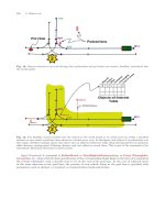
Performance of the tracker gets worse when users wear eyeglasses because different bright blobs appear
in the image due to IR reflections in the glasses, as can be seen in Fig. 6. Although the degree of reflection
on the glasses depends on its material and the relative position between the user’s head and the illuminator,
in the real tests carried out, the reflection of the inner ring of LEDs appears as a filled circle on the glasses,
of the same size and intensity as the pupil. The reflection of the outer ring appears as a circumference with
bright points around it and with similar intensity to the pupil. Some ideas for improving the tracking with
glasses are presented in Sect. 5. The system was also tested with people wearing contact lenses. In this case
no differences in the tracking were obtained compared to the drivers not wearing them.
26 L.M. Bergasa et al.
Fig. 6. System working with user wearing glasses
Fig. 7. Finite state machine for ocular measures
3.3 Visual Behaviors
Eyelid movements and face pose are some of the visual behaviors that reflect a person’s level of inattention.
There are several ocular measures to characterize sleepiness such as eye closure duration, blink frequency,
fixed gaze, eye closure/opening speed, and the recently developed parameter PERCLOS [14, 41]. This last
measure indicates the accumulative eye closure duration over time excluding the time spent on normal eye
blinks. It has been found to be the most valid ocular parameter for characterizing driver fatigue [24]. Face pose
determination is related to computation of face orientation and position, and detection of head movements.
Frequent head tilts indicate the onset of fatigue. Moreover, the nominal face orientation while driving is

frontal. If the driver faces in other directions for an extended period of time, it is due to visual distraction.
Gaze fixations occur when driver’s eyes are nearly stationary. Their fixation position and duration may relate
to attention orientation and the amount of information perceived from the fixated location, respectively.
This is a characteristic of some fatigue and cognitive distraction behaviors and it can be measured by
estimating the fixed gaze. In this work, we have measured all the explained parameters in order to evaluate
its performance for the prediction of the driver inattention state, focusing on the fatigue category.
To obtain the ocular measures we continuously track the subject’s pupils and fit two ellipses, to each of
them, using a modification of the LIN algorithm [17], as implemented in the OpenCV library [7]. The degree
of eye opening is characterized by the pupil shape. As eyes close, the pupils start getting occluded by the
eyelids and their shapes get more elliptical. So, we can use the ratio of pupil ellipse axes to characterize
the degree of eye opening. To obtain a more robust estimation of the ocular measures and, for example, to
distinguish between a blink and an error in the tracking of the pupils, we use a Finite State Machine (FSM)
as we depict in Fig. 7. Apart from the init
state, five states have been defined: tracking ok, closing, closed,
opening and tracking
lost. Transitions between states are achieved from frame to frame as a function of the
width-height ratio of the pupils.
Visual Monitoring of Driver Inattention 27
The system starts at the init state. When the pupils are detected, the FSM passes to the tracking ok state
indicating that the pupil’s tracking is working correctly. Being in this state, if the pupils are not detected in
a frame, a transition to the tracking
lost state is produced. The FSM stays in this state until the pupils are
correctly detected again. In this moment, the FSM passes to the tracking
ok state. If the width-height ratio
of the pupil increases above a threshold (20% of the nominal ratio), a closing eye action is detected and the
FSM changes to the closing
state. Because the width-height ratio may increase due to other reasons, such as
segmentation noise, it is possible to return to the tracking
ok state if the ratio does not constantly increase.
When the pupil ratio is above the 80% of its nominal size or the pupils are lost, being in closing

state,a
transition of the FSM to closed
state is provoked, which means that the eyes are closed. A new detection of the
pupils from the closed
state produces a change to opening state or tracking ok state, depending on the degree
of opening of the eyelid. If the pupil ratio is between the 20 and the 80% a transition to the opening
state is
produced, if it is below the 20% the system pass to the tracking
ok state. Being in closed state, a transition
to the tracking
lost state is produced if the closed time goes over a threshold. A transition from opening to
closing is possible if the width-height ratio increases again. Being in opening
state, if the pupil ratio is below
the 20% of the nominal ratio a transition to tracking
ok state is produced.
Ocular parameters that characterize eyelid movements have been calculated as a function of the FSM.
PERCLOS is calculated from all the states, except from the tracking
lost state, analyzing the pupil width-
height ratio. We consider that an eye closure occurs when the pupil ratio is above the 80% of its nominal
size. Then, the eye closure duration measure is calculated as the time that the system is in the closed
state.
To obtain a more robust measurement of the PERCLOS, we compute this running average. We compute
this parameter by measuring the percentage of eye closure in a 30-s window. Then, PERCLOS measure
represents the time percentage that the system is at the closed
state evaluated in 30 s and excluding the
time spent in normal eye blinks. Eye closure/opening speed measures represent the amount of time needed
to fully close the eyes or to fully open the eyes. Then, eye closure/opening speed is calculated as the time
during which pupil ratio passes from 20 to 80% or from 80 to 20% of the nominal ratio, respectively. In
other words, the time that the system is in the closing
state or opening state, respectively. Blink frequency

measure indicates the number of blinks detected in 30 s. A blink action will be detected as a consecutive
transition among the following states: closing, closed, and opening, given that this action was carried out in
less than a predefined time. Many physiology studies have been carried out on the blinking duration. We
have used the recommendation value derived in [31] but this could be easily modified to conform to other
recommended value. Respecting the eye nominal size used for the ocular parameters calculation, it varies
depending on the driver. To calculate its correct value a histogram of the eyes opening degree for the last
2,000 frames not exhibiting drowsiness is obtained. The most frequent value on the histogram is considered
to be the nominal size. PERCLOS is computed separately in both eyes and the final value is obtained as the
mean of both.
Besides, face pose can be used for detecting fatigue or visual distraction behaviors among the categories
defined for inattentive states. The nominal face orientation while driving is frontal. If the driver’s face
orientation is in other directions for an extended period of time it is due to visual distractions, and if it
occurs frequently (in the case of various head tilts), it is a clear symptom of fatigue. In our application, the
precise degree of face orientation for detecting this behaviors is not necessary because face poses in both
cases are very different from the frontal one. What we are interested in is to detect whether the driver’s head
deviates too much from its nominal position and orientation for an extended period of time or too frequently
(nodding detection).
This work provides a novel solution to the coarse 3D face pose estimation using a single un-calibrated
camera, based on the method proposed in [37]. We use a model-based approach for recovering the face pose
by establishing the relationship between 3D face model and its two-dimensional (2D) projections. A weak
perspective projection is assumed so that face can be approximated as a planar object with facial features,
such as eyes, nose and mouth, located symmetrically on the plane. We have performed a robust 2D face
tracking based on the pupils and the nostrils detections on the images. Nostrils detection has been carried
out in a way similar to that used for the pupils’ detection. From these positions the 3D face pose is estimated,
and as a function of it, face direction is classified in nine areas, from upper left to lower right.
28 L.M. Bergasa et al.
This simple technique works fairly well for all the faces we tested, with left and right rotations specifically.
A more detailed explanation about our method was presented by the authors in [5]. As the goal is to detect
whether the face pose of the driver is not frontal for an extended period of time, this has been computed
using only a parameter that gives the percentage of time that the driver has been looking at the front, over

a 30-s temporal window.
Nodding is used to quantitatively characterize one’s level of fatigue. Several systems have been reported
in the literature to calculate this parameter from a precise estimation of the driver’s gaze [23, 25]. However,
these systems have been tested in laboratories but not in real moving vehicles. The noise introduced in real
environments makes these systems, based on exhaustive gaze calculation, work improperly. In this work, a
new technique based on position and speed data from the Kalman filters used to track the pupils and the
FSM is proposed. This parameter measures the number of head tilts detected in the last 2 min. We have
experimentally observed that when a nodding is taking place, the driver closes his or her eyes and the head
goes down to touch the chest or the shoulders. If the driver wakes up in that moment, raising his head, the
values of the vertical speed of the Kalman filters will change their sign, as the head rises. If the FSM is in
closed
state or in tracking lost and the pupils are detected again, the system saves the speeds of the pupils
trackers for ten frames. After that, the data is analyzed to find if it conforms to that of a nodding. If so, the
first stored value is saved and used as an indicator of the “magnitude” of the nodding.
Finally, one of the remarkable behaviors that appear in drowsy drivers or cognitively distracted drivers
is fixed gaze. A fatigued driver looses the focus of the gaze, not paying attention to any of the elements of
the traffic. This loss of concentration is usually correlated with other sleepy behaviors such as a higher blink
frequency, a smaller degree of eye opening and nodding. In the case of cognitive distraction, however, fixed
gaze is decoupled from other clues. As for the parameters explained above, the existing systems calculate this
parameter from a precise estimation of the driver’s gaze and, consequently, experience the same problems. In
order to develop a method to measure this behavior in a simple and robust way, we present a new technique
based on the data from the Kalman filters used to track the pupils.
An attentive driver moves his eyes frequently, focusing to the changing traffic conditions, particularly
if the road is busy. This has a clear reflection on the difference between the estimated position from the
Kalman filters and the measured ones.
Besides, the movements of the pupils for an inattentive driver present different characteristics. Our system
monitors the position on the x coordinate. Coordinate y is not used, as the difference between drowsy and
awake driver is not so clear. The fixed gaze parameter is computed locally over a long period of time, allowing
for freedom of movement of the pupil over time. We refer here to [5] for further details of the computation
of this parameter.

This fixed gaze parameter may suffer from the influence of vehicle vibrations or bumpy roads. Modern
cars have reduced vibrations to a point that the effect is legible on the measure. The influence of bumpy roads
depends on their particular characteristics. If bumps are occasional, it will only affect few values, making
little difference in terms of the overall measure. On the other hand, if bumps are frequent and their magnitude
is high enough, the system will probably fail to detect this behavior. Fortunately, the probability for a driver
to get distracted or fall asleep is significantly lower in very bumpy roads. The results obtained for all the
test sequences with this parameter are encouraging. In spite of using the same a priori threshold for different
drivers and situations, the detection was always correct. Even more remarkable was the absence of false
positives.
3.4 Driver Monitoring
This section describes the method to determine the driver’s visual inattention level from the parameters
obtained in the previous section. This process is complicated because several uncertainties may be present.
First, fatigue and cognitive distractions are not observable and they can only be inferred from the available
information. In fact, this behavior can be regarded as the result of many contextual variables such as
environment, health, and sleep history. To effectively monitor it, a system that integrates evidences from
multiple sensors is needed. In the present work, several fatigue visual behaviors are subsequently combined
to form an inattentiveness parameter that can robustly and accurately characterize one’s vigilance level.
Visual Monitoring of Driver Inattention 29
The fusion of the parameters has been obtained using a fuzzy system. We have chosen this technique for its
well known linguistic concept modeling ability. Fuzzy rule expressions are close to expert natural language.
Then, a fuzzy system manages uncertain knowledge and infers high level behaviors from the observed data.
As an universal approximator, fuzzy inference system can be used for knowledge induction processes. The
objective of our fuzzy system is to provide a driver’s inattentiveness level (DIL) from the fusion of several
ocular and face pose measures, along with the use of expert and induced knowledge. This knowledge has
been extracted from the visual observation and the data analysis of the parameters in some simulated fatigue
behavior carried out in real conditions (driving a car) with different users. The simulated behaviors have
been done according to the physiology study of the US Department of Transportation, presented in [24].
We do not delve into the psychology of driver visual attention, rather we merely demonstrate that with the
proposed system, it is possible to collect driver information data and infer whether the driver is attentive
or not.

The first step in the expert knowledge extraction process is to define the number and nature of the vari-
ables involved in the diagnosis process according to the domain expert experience. The following variables are
proposed after appropriate study of our system: PERCLOS, eye closure duration, blink frequency, nodding
frequency, fixed gaze and frontal face pose. Eye closing and opening variables are not being used in our input
fuzzy set because they mainly depend on factors such as segmentation and correct detection of the eyes, and
they take place in the length of time comparable to that of the image acquisition. As a consequence, they
are very noisy variables. As our system is adaptive to the user, the ranges of the selected fuzzy inputs are
approximately the same for all users. The fuzzy inputs are normalized, and different linguistic terms and its
corresponding fuzzy sets are distributed in each of them using induced knowledge based on the hierarchical
fuzzy partitioning (HFP) method [20]. Its originality lies in not yielding a single partition, but a hierarchy
including partitions with various resolution levels based on automatic clustering data. Analyzing the fuzzy
partitions obtained by HFP, we determined that the best suited fuzzy sets and the corresponding linguistic
terms for each input variable are those shown in Table 1. For the output variable (DIL), the fuzzy set and
the linguistic terms were manually chosen. The inattentiveness level range is between 0 and 1, with a normal
value up to 0.5. When its value is between 0.5and0.75, driver’s fatigue is medium, but if the DIL is over
0.75 the driver is considered to be fatigued, and an alarm is activated. Fuzzy sets of triangular shape were
chosen, except at the domain edges, where they were semi-trapezoidal.
Based on the above selected variables, experts state different pieces of knowledge (rules) to describe certain
situations connecting some symptoms with a certain diagnosis. These rules are of the form “If condition,
Then conclusion”, where both premise and conclusion use the linguistic terms previously defined, as in the
following example:
• IF PERCLOS is large AND Eye Closure Duration is large, THEN DIL is large
In order to improve accuracy and system design, automatic rule generation and its integration in the
expert knowledge base were considered. The fuzzy system implementation used the licence-free tool Knowl-
edge Base Configuration Tool (KBCT) [2] developed by the Intelligent Systems Group of the Polytechnics
University of Madrid (UPM). A more detailed explanation of this fuzzy system can be found in [5].
Tabl e 1. Fuzzy variables
Variable Type Range Labels Linguistic terms
PERCLOS In [0.0, 1.0] 5 Small, medium small, medium, medium large, large
Eye closure duration In [1.0–30.0] 3 Small, medium, large

Blink freq. In [1.0–30.0] 3 Small, medium, large
Nodding freq. In [0.0–8.0] 3 Small, medium, large
Face position In [0.0–1.0] 5 Small, medium small, medium, medium large, large
Fixed gaze In [0.0–0.5] 5 Small, medium small, medium, medium large, large
DIL Out [0.0–1.0] 5 Small, medium small, medium, medium large, large
30 L.M. Bergasa et al.
4 Experimental Results
The goal of this section is to experimentally demonstrate the validity of our system in order to detect fatigue
behaviors in drivers. Firstly, we show some details about the recorded video sequences used for testing, then,
we analyze the parameters measured for one of the sequences. Finally, we present the performance of the
detection of each one of the parameters, and the overall performance of the system.
4.1 Test Sequences
Ten sequences were recorded in real driving situations over a highway and a two-direction road. Each sequence
was obtained for a different user. The images were obtained using the system explained in Sect. 3.1. The
drivers simulated some drowsy behaviors according to the physiology study of the US Department of Trans-
portation presented in [24]. Each user drove normally except in one or two intervals where the driver simulated
fatigue. Simulating fatigue allows for the system to be tested in a real motorway, with all the sources of noise
a deployed system would face. The downside is that there may be differences between an actual drowsy
driver and a driver mimicking the standard drowsy behavior, as defined in [24]. We are currently working
on testing the system in a truck simulator.
The length of the sequences and the fatigue simulation intervals are shown in Table 2. All the sequences
were recorded at night except for sequence number 7 that was recorded at day, and sequence number 5
that was recorded at sunset. Sequences were obtained with different drivers not wearing glasses, with the
exception of sequence 6, that was recorded for testing the influence of the glasses in real driving conditions.
4.2 Parameter Measurement for One of the Test Sequences
The system is currently running on a PC Pentium4 (1.8 Ghz) with Linux kernel 2.6.18 in real time (25 pairs
of frames/s) with a resolution of 640×480 pixels. Average processing time per pair of frames is 11.43 ms.
Figure 8 depicts the parameters measured for sequence number 9. This is a representative test example with
a duration of 465 s where the user simulates two fatigue behaviors separated by an alertness period. As can
be seen, until second 90, and between the seconds 195 and 360, the DIL is below 0.5 indicating an alertness

state. In these intervals the PERCLOS is low (below 0.15), eye closure duration is low (below the 200 ms),
blink frequency is low (below two blinks per 30-s window) and nodding frequency is zero. These ocular
parameters indicate a clear alert behavior. The frontal face position parameter is not 1.0, indicating that
the predominant position of the head is frontal, but that there are some deviations near the frontal position,
typical of a driver with a high vigilance level. The fixed gaze parameter is low because the eyes of the driver
are moving caused by a good alert condition. DIL increases over the alert threshold during two intervals
(from 90 to 190 and from 360 to 565 s) indicating two fatigue behaviors. In both intervals the PERCLOS
increases from 0.15 to 0.4, the eye closure duration goes up to 1,000 ms, and the blink frequency parameter
Tabl e 2. Length of simulated drowsiness sequences
Seq. Num. Drowsiness behavior time (s) Alertness behavior time (s) Total time (s)
1 394 (two intervals: 180 + 214) 516 910
2 90 (one interval) 210 300
3 0 240 240
4 155 (one interval) 175 330
5 160 (one interval) 393 553
6 180 (one interval) 370 550
7 310 (two intervals: 150 + 160) 631 941
8 842 (two intervals: 390 + 452) 765 1,607
9 210 (two intervals: 75 + 135) 255 465
10 673 (two intervals: 310 + 363) 612 1,285
Visual Monitoring of Driver Inattention 31
Fig. 8. Parameters measured for the test sequence number 9
Tabl e 3. Parameter measurement performance
Parameters Total % correct
PERCLOS 93.1
Eye closure duration 84.4
Blink freq. 79.8
Nodding freq. 72.5
Face pose 87.5
Fixed gaze 95.6

increases from 2 to 5 blinks. The frontal face position is very close to 1.0 because the head position is fixed
and frontal. The fixed gaze parameter increases its value up to 0.4 due to the narrow gaze in the line of sight
of the driver. This last variation indicates a typical loss of concentration, and it takes place before other
sleepy parameters could indicate increased sleepiness, as can be observed. The nodding is the last fatigue
effect to appear. In the two fatigue intervals a nodding occurs after the increase of the other parameters,
indicating a low vigilance level. This last parameter is calculated over a temporal window of 2 min, so its
value remains stable most of the time.
This section described an example of parameter evolution for two simulated fatigue behaviors of one
driver. Then, we analyzed the behaviors of other drivers in different circumstances, according to the video
tests explained above. The results obtained are similar to those shown for sequence number 9. Overall results
of the system are explained in what follows.
4.3 Parameter Performance
The general performance of the measured parameters for a variety of environments with different drivers,
according to the test sequences, is presented in Table 3. Performance was measured by comparing the
algorithm results to results obtained by manually analyzing the recorded sequences on a frame-by-frame
basis. Each frame was individually marked with the visual behaviors the driver exhibited, if any. Inaccuracies
of this evaluation can be considered negligible for all parameters. Eye closure duration is not easy to evaluate
accurately, as the duration of some quick blinks is around 5–6 frames at the rate of 25 frames per second
(fps), and the starting of the blink can fall between two frames. However, the number of quick blinks is not
big enough to make further statistical analysis necessary.
For each parameter the total correct percentage for all sequences excluding sequence number 6 (driver
wearing glasses) and sequence number 7 (recorded during the day) is depicted. Then, this column shows
the parameter detection performance of the system for optimal situations (driver without glasses driving at
32 L.M. Bergasa et al.
night). The performance gets considerably worse by day and it dramatically decreases when drivers wear
glasses.
PERCLOS results are quite good, obtaining a total correct percentage of 93.1%. It has been found to
be a robust ocular parameter for characterizing driver fatigue. However, it may fail sometimes, for example,
when a driver falls asleep without closing her eyes. Eye closure duration performance (84.4%) is a little worse
than that of the PERCLOS, because the correct estimation of the duration is more critical. The variation

on the intensity when the eye is partially closed with regard to the intensity when it is open complicates the
segmentation and detection. This causes the frame count for this parameter to be usually less than the real
one. These frames are considered as closed time. Measured time is slightly over the real time, as a result
of delayed detection. Performance of blink frequency parameter is about 80% because some quick blinks
are not detected at 25 fps. Then, the three explained parameters are clearly correlated almost linearly, and
PERCLOS is the most robust and accurate one.
Nodding frequency results are the worst (72.5%), as the system is not sensible to noddings in which
the driver rises her head and then opens her eyes. To reduce false positives, the magnitude of the nodding
(i.e., the absolute value of the Kalman filter speed), must be over a threshold. In most of the non-detected
noddings, the mentioned situation took place, while the magnitude threshold did not have any influence on
any of them. The ground truth for this parameter was obtained manually by localizing the noddings on the
recorded video sequences. It is not correlated with the three previous parameters, and it is not robust enough
for fatigue detection. Consequently, it can be used as a complementary parameter to confirm the diagnosis
established based on other more robust methods.
The evaluation of the face direction provides a measure of alertness related to drowsiness and visual
distractions. This parameter is useful for both detecting the pose of the head not facing the front direction
and the duration of the displacement. The results can be considered fairly good (87.5%) for a simple model
that requires very little computation and no manual initialization. The ground truth in this case was obtained
by manually looking for periods in which the driver is not clearly looking in front in the video sequences,
and comparing their length to that of the periods detected by the system. There is no a clear correlation
between this parameter and the ocular ones for fatigue detection. This would be the most important cue in
case of visual distraction detection.
Performance of the fixed gaze monitoring is the best of the measured parameters (95.6%). The maxi-
mum values reached by this parameter depend on users’ movements and gestures while driving, but a level
above 0.05 is always considered to be an indicator of drowsiness. Values greater than 0.15 represent high
inattentiveness probability. These values were determined experimentally. This parameter did not have false
positives and is largely correlated with the frontal face direction parameter. On the contrary, it is not clearly
correlated with the rest of the ocular measurements. For cognitive distraction analysis, this parameter would
be the most important cue, as this type of distraction does not normally involve head or eye movements.
The ground truth for this parameter was manually obtained by analyzing eye movements frame by frame

for the intervals where a fixed gaze behavior was being simulated. We can conclude from these data that
fixed gaze and PERCLOS are the most reliable parameters for characterizing driver fatigue, at least for our
simulated fatigue study.
All parameters presented in Table 3 are fused in the fuzzy system to obtain the DIL for final evaluation
of sleepiness. We compared the performance of the system using only the PERCLOS parameter and the
DIL(using all of the parameters), in order to test the improvements of our proposal with respect to the
most widely used parameter for characterizing driver drowsiness. The system performance was evaluated by
comparing the intervals where the PERCLOS/DIL was above a certain threshold to the intervals, manually
analyzed over the video sequences, in which the driver simulates fatigue behaviors. This analysis consisted
of a subjective estimation of drowsiness by human observers, based on the Wierwille test [41].
As can be seen in Table 4, correct detection percentage for DIL is very high (97%). It is higher than the
obtained using only PERCLOS, for which the correct detection percentage is about the 90% for our tests.
This is due to the fact that fatigue behaviors are not the same for all drivers. Further, parameter evolution
and absolute values from the visual cues differ from user to user. Another important fact is the delay between
the moment when the driver starts his fatigue behavior simulation and when the fuzzy system detects it.
This is a consequence of the window spans used in parameter evaluation. Each parameter responds to a
Visual Monitoring of Driver Inattention 33
Tabl e 4. Sleepiness detection performance
Parameter Total % correct
PERCLOS 90
DIL 97
different stage in the fatigue behavior. For example, fixed gaze behavior appears before PERCLOS starts
to increase, thus rising the DIL to a value where a noticeable increment of PERCLOS would rise an alarm
in few seconds. This is extensible to the other parameters. Using only the PERCLOS would require much
more time to activate an alarm (tens of seconds), especially if the PERCLOS increases more slowly for some
drivers. Our system provides an accurate characterization of a driver’s level of fatigue, using multiple visual
parameters to resolve the ambiguity present in the information from a single parameter. Additionally, the
system performance is very high in spite of the partial errors associated to each input parameter. This was
achieved using redundant information.
5 Discussion

It has been shown that the system’s weaknesses can be almost completely attributed to the pupil detection
strategy, because it is the most sensitive to external interference. As it has been mentioned above, there are
a series of situations where the pupils are not detected and tracked robustly enough. Pupil tracking is based
on the “bright pupil” effect, and when this effect does not appear clearly enough on the images, the system
can not track the eyes. Sunlight intensity occludes the near-IR reflected from the driver’s eyes. Fast changes
in illumination that the Automatic Gain Control in the camera can not follow produce a similar result. In
both cases the “bright pupil” effect is not noticeable in the images, and the eyes can not be located. Pupils
are also occluded when the driver’s eyes are closed. It is then not possible to track the eyes if the head
moves during a blink, and there is an uncertainty of whether the eyes may still be closed or they may have
opened and appeared in a position on the image far away from where they were a few frames before. In this
situation, the system would progressively extend the search windows and finally locate the pupils, but in
this case the measured duration of the blink would not be correct. Drivers wearing glasses pose a different
problem. “Bright pupil” effect appears on the images, but so do the reflections of the LEDs from the glasses.
These reflections are very similar to the pupil’s, making detection of the correct one very difficult.
We are exploring alternative approaches to the problem of pupil detection and tracking, using methods
that are able to work 24/7 and in real time, and that yield accurate enough results to be used in other
modules of the system. A possible solution is to use an eye or face tracker that does not rely on the “bright
pupil” effect. Also, tracking the whole face, or a few parts of it, would make it possible to follow its position
when eyes are closed, or occluded.
Face and eye location is an extensive field in computer vision, and multiple techniques have been devel-
oped. In recent years, probably the most successful have been texture-based methods and machine learning.
A recent survey that compares some of these methods for eye localization can be found in [8]. We have
explored the feasibility of using appearance (texture)-based methods, such as Active Appearance Models
(AAM) [9]. AAM are generative models, that try to parameterize the contents of an image by generating a
synthetic image as close as possible to the given one. The synthetic image is obtained from a model consisting
of both appearance and shape. These appearance and shape are learned in a training process, and thus can
only represent a constrained range of possible appearances and deformations. They are represented by a
series of orthogonal vectors, usually obtained using Principal Component Analysis (PCA), that form a base
in the appearance and deformation spaces.
AAMs are linear in both shape and appearance, but are nonlinear in terms of pixel intensities. The shape

of the AAM is defined as the coordinates of the v vertices of the shape
s =(x
1
,y
1
,x
2
,y
2
, ··· ,x
v
,y
v
)
t
(1)
34 L.M. Bergasa et al.
0 50 100 150 200 250 300 350
0
50
100
150
200
250
300
350
400
Fig. 9. A triangulated shape
and can be instantiated from the vector base simply as:
s = s

0
+
n

i=1
p
i
· s
i
(2)
where s
0
is the base shape and s
i
are the shape vectors. Appearance is instantiated in the same way
A(x)=A
0
(x)+
m

i=1
λ
i
· A
i
(x)(3)
where A
0
(x)isthebase appearance, A
i

(x)aretheappearance vectors and λ
i
are the weights of these vectors.
The final model instantiation is obtained by warping the appearance A(x), whose shape is s
0
,soit
conforms to the shape s. This is usually done by triangulating the vertices of the shape, using Delaunay [13]
or another triangulation algorithm, as shown in Fig. 9. The appearance that falls in each triangle is affine
warped independently, accordingly to the position of the vertices of the triangle in s
0
and s.
The purpose of fitting the model to a given image is to obtain the parameters that minimize the error
between the image I and the model instance:

x∈s
0

A
0
(x)+
m

i=1
λ
i
A
i
(x) −I(W(x; p))

2

(4)
where W(x; p) is a warp defined over the pixel positions x by the shape parameters p.
These parameters can be then analyzed to gather interesting data, in our case, the position of the eyes
and head pose. Minimization is done using the Gauss–Newton method, or some efficient variations, such as
the inverse compositional algorithm [4, 28].
We tested the performance and robustness of the Active Appearance Models on the same in-car sequences
described above. AAMs perform well in sequences where the IR-based system did not, such as sequence 6,
where the driver is wearing glasses (Figs. 10a,b), and is able to work with sunlight (10c), and track the face
under fast illumination changes (10d–f). Also, as the model covers most of the face, the difference between
a blink and a tracking loss is clearer, as the model can be fitted when eyes are either open or closed.
On our tests, however, AAM was only fitted correctly when the percentage of occlusion (or self-occlusion,
due to head turns) of the face was below 35% of the face. It was also able to fit with low error although the
position of the eyes was not determined with the required precision (i.e., the triangles corresponding to the
pupil were positioned closer to the corner of the eye than to the pupil). The IR-based system could locate
and track an eye when the other eye was occluded, which the AAM-based system is not able to do. More
detailed results can be found on [30].
Overall results of face tracking and eye localization with AAM are encouraging, but the mentioned
shortcomings indicate that improved robustness is necessary. Constrained Local Models (CLM) are models
closely related to AAM, that have shown improved robustness and accuracy [10]. Instead of covering the
whole face, CLM only use small rectangular patches placed in specific points that are interesting for its
characteristic appearance or high contrast. Constrained Local Models are trained in the same way as AAMs,
and both a shape and appearance vector bases are obtained.
Visual Monitoring of Driver Inattention 35
(a) (b) (c)
(d) (e) (f)
Fig. 10. Fitting results with glasses and sunlight
Fig. 11. A constrained local model fitted over a face
Fitting the CLM to an image is done in two steps. First, the same minimization that was used for AAMs
is performed, with the difference that now no warping is applied over the rectangles. Those are only displaced
over the image. In the second step, the correlation between the patches and the image is maximized, with

an iterative algorithm, typically the Nelder–Mead simplex algorithm [29].
The use of small patches and the two-step fitting algorithm make CLM more robust and efficient
than AAM. See Fig. 11 for an example. The CLM is a novel technique that performs well in controlled
environments, but that has to be thoroughly tested in challenging operation scenarios.
6 Conclusions and Future Work
We have developed a non-intrusive prototype computer vision system for real-time monitoring of driver’s
fatigue. It is based on a hardware system for real time acquisition of driver’s images using an active IR illu-
minator and the implementation of software algorithms for real-time monitoring of the six parameters that
36 L.M. Bergasa et al.
better characterize the fatigue level of a driver. These visual parameters are PERCLOS, eye closure duration,
blink frequency, nodding frequency, face pose and fixed gaze. In an attempt to effectively monitor fatigue,
a fuzzy classifier was implemented to merge all these parameters into a single Driver Inattentiveness Level.
Monitoring distractions (both visual and cognitive) would be possible using this system. The system devel-
opment has been discussed. The system is fully autonomous, with automatic (re)initializations if required.
It was tested with different sequences recorded in real driving condition with different users during several
hours. In each of them, several fatigue behaviors were simulated during the test. The system works robustly
at night for users not wearing glasses, yielding accuracy of 97%. Performance of the system decreases during
the daytime, especially in bright days, and at the moment it does not work with drivers wearing glasses. A
discussion about improvements of the system in order to overcome these weaknesses has been included.
The results and conclusions obtained support our approach to the drowsiness detection problem. In the
future the results will be completed with actual drowsiness data. We have the intention of testing the system
with more users for long periods of time, to obtain real fatigue behaviors. With this information we will
generalize our fuzzy knowledge base. Then, we would like to improve our vision system with some of the
techniques mentioned in the previous section, in order to solve the problems of daytime operation and to
improve the solution for drivers wearing glasses. We also plan to add two new sensors (a steering wheel sensor
and a lane tracking sensor) for fusion with the visual information to achieve correct detection, especially at
daytime.
Acknowledgements
This work has been supported by grants TRA2005-08529-C02-01 (MOVICON Project) and PSE-370100-
2007-2 (CABINTEC Project) from the Spanish Ministry of Education and Science (MEC). J. Nuevo is also

working under a researcher training grant from the Education Department of the Comunidad de Madrid and
the European Social Fund.
References
1. Inc. Agilent Technologies. Application Note 1118: Compliance of Infrared Communication Products to IEC 825-1
and CENELEC EN 60825-1, 1999.
2. J.M. Alonso, S. Guillaume, and L. Magdalena. KBCT, knowledge base control tool, 2003. URL
/>3. Anon. Perclos and eyetracking: Challenge and opportunity. Technical report, Applied Science Laboratories,
Bedford, MA, 1999. URL
4. S. Baker and I. Matthews. Lucas-Kanade 20 years on: A unifying framework. International Journal of Computer
Vision, 56(3):221–255, March 2004.
5. L.M. Bergasa, J. Nuevo, M.A. Sotelo, R. Barea, and M.E. Lopez. Real-time system for monitoring driver vigilance.
Intelligent Transportation Systems, IEEE Transactions on Intelligent Transportation Systems, 7(1):63–77, 2006.
6. S. Boverie, J.M. Leqellec, and A. Hirl. Intelligent systems for video monitoring of vehicle cockpit. In International
Congress and Exposition ITS. Advanced Controls and Vehicle Navigation Systems, pp. 1–5, 1998.
7. G. Bradski, A. Kaehler, and V. Pisarevsky. Learning-based computer vision with intel’s open source computer
vision library. Intel Technology Journal, 09(02), May 2005.
8. P. Campadelli, R. Lanzarotti, and G. Lipori. Eye localization: a survey. In NATO Science Series, 2006.
9. T.F. Cootes, G.J. Edwards, and C.J. Taylor. Active appearance models. IEEE Transaction on Pattern Analysis
an Machine Intelligence, 23:681–685, 2001.
10. D. Cristinacce and T. Cootes. Feature Detection and Tracking with Constrained Local Models. Proceedings of
the British Machine Vision Conf, 2006.
11. DaimerChryslerAG. The electronic drawbar, June 2001. URL
12. DaimlerChrysler. Driver assistant with an eye for the essentials. URL />13. B. Delaunay. Sur la sphere vide. Izv. Akad. Nauk SSSR, Otdelenie Matematicheskii i Estestvennyka Nauk,7:
793–800, 1934.
14. D. Dinges and F. Perclos: A valid psychophysiological measure of alertness as assesed by psychomotor vigilance.
Technical Report MCRT-98-006, Federal Highway Administration. Office of motor carriers, 1998.
Visual Monitoring of Driver Inattention 37
15. European Project FP6 (IST-1-507674-IP). AIDE – Adaptive Integrated Driver-Vehicle Interface, 2004–2008. URL
/>16. European Project FP6 (IST-2002-2.3.1.2). Advanced sensor development for attention, stress, vigilance and
sleep/wakefulness monitoring (SENSATION), 2004–2007. URL

17. A.W. Fitzgibbon and R.B. Fisher. A buyer’s guide to conic fitting. In Proceedings of the 6th British Conference
on Machine Vision, volume 2, pp. 513–522, Birmingham, United Kingdom, 1995.
18. D.A. Forsyth and J. Ponce. Computer Vision: A Modern Approach. Prentice Hall, 2003.
19. R. Grace. Drowsy driver monitor and warning system. In International Driving Symposium on Human Factors
in Driver Assessment, Training and Vehicle Design, Aug 2001.
20. S. Guillaume and B. Charnomordic. A new method for inducing a set of interpretable fuzzy partitions and fuzzy
inference systems from data. Studies in Fuzziness and Soft Computing, 128:148–175, 2003.
21. H. Ueno, M. Kaneda, and M. Tsukino. Development of drowsiness detection system. In Proceedings of Vehicle
Navigation and Information Systems Conference, pp. 15–20, 1994.
22. AWAKE Consortium (IST 2000-28062). System for Effective Assessment of Driver Vigilance and Warning
According to Traffic Risk Estimation – AWAKE, Sep 2001–2004. URL
23. Q. Ji and X. Yang. Real-time eye, gaze and face pose tracking for monitoring driver vigilance. Real-Time Imaging,
8:357–377, Oct 2002.
24. A. Kircher, M. Uddman, and J. Sandin. Vehicle control and drowsiness. Technical Report VTI-922A, Swedish
National Road and Transport Research Institute, 2002.
25. D. Koons and M. Flicker. IBM Blue Eyes project, 2003. URL />26. M. Kutila. Methods for Machine Vision Based Driver Monitoring Applications. Ph.D. thesis, VTT Technical
Research Centre of Finland, 2006.
27. Y. Matsumoto and A. Zelinsky. An algorithm for real-time stereo vision implementation of head pose and gaze
direction measurements. In Proceedings of IEEE 4th International Conference Face and Gesture Recognition,
pp. 499–505, Mar 2000.
28. I. Matthews and S. Baker. Active appearance models revisited. International Journal of Computer Vision,
60(2):135–164, November 2004.
29. J.A. Nelder and R. Mead. A simplex method for function minimization. Computer Journal, 7(4):308–313, 1965.
30. J. Nuevo, L.M. Bergasa, M.A. Sotelo, and M. Ocana. Real-time robust face tracking for driver monitoring.
Intelligent Transportation Systems Conference, 2006. ITSC’06. IEEE, pp. 1346–1351, 2006.
31. L. Nunes and M.A. Recarte. Cognitive demands of hands-free phone conversation while driving, Chap. F5, pp. 133–
144. Pergamon, Oxford, 2002.
32. P. Rau. Drowsy driver detection and warning system for commercial vehicle drivers: Field operational test design,
analysis and progress, NHTSA, 2005.
33. D. Royal. Volume I – Findings; National Survey on Distracted and Driving Attitudes and Behaviours, 2002.

Technical Report DOT HS 809 566, The Gallup Organization, March 2003.
34. Seeing Machines. Facelab transport, August 2006. URL />35. Seeing Machines. Driver state sensor, August 2007. URL />36. W. Shih and Liu. A calibration-free gaze tracking technique. In Proceedings of 15th Conference Patterns
Recognition, volume 4, pp. 201–204, Barcelona, Spain, 2000.
37. P. Smith, M. Shah, and N.Da.V. Lobo. Determining driver visual attention with one camera. IEEE Transaction
on Intelligent Transportation Systems, 4(4):205–218, 2003.
38. T. Victor, O. Blomberg, and A. Zelinsky. Automating the measurement of driver visual behaviours using pas-
sive stereo vision. In Proceedings of Intelligent Conference Series Vision in Vehicles VIV9, Brisbane, Australia,
Aug 2001.
39. Volvo Car Corporation. Driver alert control. URL
40. W. Wierwille, L. Tijerina, S. Kiger, T. Rockwell, E. Lauber, and A. Bittne. Final report supplement – task 4:
Review of workload and related research. Technical Report DOT HS 808 467(4), USDOT, Oct 1996.
41. W. Wierwille, Wreggit, Kirn, Ellsworth, and Fairbanks. Research on vehicle-based driver status/performance
monitoring; development, validation, and refinement of algorithms for detection of driver drowsiness, final report;
technical reports & papers. Technical Report DOT HS 808 247, USDOT, Dec 1994. URL www.its.dot.gov
Understanding Driving Activity Using Ensemble Methods
Kari Torkkola, Mike Gardner, Chris Schreiner, Keshu Zhang, Bob Leivian, Harry Zhang,
and John Summers
Motorola Labs, Tempe, AZ 85282, USA,
1 Introduction
Motivation for the use of statistical machine learning techniques in the automotive domain arises from our
development of context aware intelligent driver assistance systems, specifically, Driver Workload Management
systems. Such systems integrate, prioritize, and manage information from the roadway, vehicle, cockpit,
driver, infotainment devices, and then deliver it through a multimodal user interface. This could include
incoming cell phone calls, email, navigation information, fuel level, and oil pressure to name a very few. In
essence, the workload manager attempts to get the right information to the driver at the right time and in
the right way in order that driver performance is optimized and distraction is minimized.
In order to do its job, the workload manager system needs to track the wider driving context including
the state of the roadway, traffic conditions, and the driver. Current automobiles have a large number of
embedded sensors, many of which produce data that are available through the car data bus. The state
of many on-board and carried-in devices in the cockpit is also available. New advanced sensors, such as

video-based lane departure warning systems and radar-based collision warning systems are currently being
deployed in high end car models. All of these could be used to define the driving context [17]. But a number
of questions arise:
• What are the range of typical driving maneuvers, as well as near misses and accidents, and how do drivers
navigate them?
• Under what conditions does driver performance degrade or driver distraction increase?
• What are the optimal set of sensors and algorithms that can recognize each of these driving conditions
near the theoretical limit for accuracy, and what is the sensor set that are accurate yet cost effective?
There are at least two approaches to address these questions. The first is more or less heuristic: experts
offer informed opinions on the various matters and sets of sensors are selected accordingly with algorithms
coded using rules of thumb. Individual aspects of the resulting system are tested by using narrow human
factors testing controlling all but a few variables. Hundreds of iterations must be completed in order to
test the impact on driver performance of the large combinations of driving states, sensor sets, and various
algorithms.
The second approach, which we advocate in this chapter and in [28], involves using statistical machine
learning techniques that enable the creation of new human factors approaches. Rather than running large
numbers of narrowly scoped human factors testing with only a few variables, we chose to invent a “Hypervari-
ate Human Factors Test Methodology” that uses broad naturalistic driving experiences that capture wide
conditions resulting in hundreds of variables, but decipherable with machine learning techniques. Rather
than pre-selecting our sensor sets we chose to collect data from every sensor we could think of and some not
yet invented that might remotely be useful by creating behavioral models overlaid with our vehicle system.
Furthermore, all sensor outputs were expanded by standard mathematical transforms that emphasized vari-
ous aspects of the sensor signals. Again, data relationships are discoverable with machine learning. The final
K. Torkkola et al.: Understanding Driving Activity Using Ensemble Methods, Studies in Computational Intelligence (SCI) 132, 39–58
(2008)
www.springerlink.com
c
 Springer-Verlag Berlin Heidelberg 2008
40 K. Torkkola et al.
data set consisted of hundreds of driving hours with thousands of variable data outputs which would have

been nearly impossible to annotate without machine learning techniques.
In this chapter we describe three major efforts that have employed our machine learning approach. First,
we discuss how we have utilized our machine learning approach to detect and classify a wide range of driving
maneuvers, and describe a semi-automatic data annotation tool we have created to support our modeling
effort. Second, we perform a large scale automotive sensor selection study towards intelligent driver assistance
systems. Finally, we turn our attention to creating a system that detects driver inattention by using sensors
that are available in the current vehicle fleet (including forwarding looking radar and video-based lane
departure system) instead of head and eye tracking systems.
This approach resulted in the creation of two generations of our workload manager system called Driver
Advocate, Driver Advocate that was based on data rather than just expert opinions. The described techniques
helped reduce the research cycle times while resulting in broader insight. There was rigorous quantification of
theoretical sensor subsystem performance limits and optimal subsystem choices given economic price points.
The resulting system performance specs and architecture design created a workload manager that had a
positive impact on driver performance [23, 33].
2 Modeling Naturalistic Driving
Having the ability to detect driving maneuvers can be of great benefit in determining a driver’s current
workload state. For instance, a driving workload manager may decide to delay presenting the driver with
non-critical information if the driver was in the middle of a complex driving maneuver. In this section we
describe our data-driven approach to classifying driving maneuvers.
There are two approaches to collecting large databases of driving sensor data from various driving sit-
uations. One can outfit a fleet of cars with sensors and data collection equipment, as has been done in the
NHTSA 100-car study [18]. This has the advantage of being as naturalistic as possible. However, the disad-
vantage is that potentially interesting driving situations will be extremely rare in the collected data. Realistic
driving simulators provide much more controlled environments for experimentation and permit the creation
of many interesting driving situations within a reasonable time frame. Furthermore, in a driving simulator,
it is possible to simulate a large number of potential advanced sensors that would be yet too expensive or
impossible to install in a real car. This will also enable us to study what sensors really are necessary for
any particular task and what kind of signal processing of those sensors is needed in order to create adequate
driving situation models based on those sensors.
We collect data in a driving simulator lab, which is an instrumented car in a surround video virtual world

with full visual and audio simulation (although no motion or G-force simulation) of various roads, traffic and
pedestrian activity. The driving simulator consists of a fixed based car surrounded by five front and three
rear screens (Fig. 1). All driver controls such as the steering wheel, brake, and accelerator are monitored
and affect the motion through the virtual world in real-time. Various hydraulics and motors provide realistic
force feedback to driver controls to mimic actual driving.
The basic driving simulator software is a commercial product with a set of simulated sensors that,
at the behavioral level, simulate a rich set of current and near future on-board sensors (http://www.
drivesafety.com). This set consists of a radar for locating other traffic, a GPS system for position infor-
mation, a camera system for lane positioning and lane marking detection, and a mapping data base for
road names, directions, locations of points of interest, etc. There is also a complete car status system for
determining the state of engine parameters (coolant temperature, oil pressure, etc.) and driving controls
(transmission gear selection, steering angle, gas pedal, brake pedal, turn signal, window and seat belt status,
etc.). The simulator setup also has several video cameras, microphones, and infrared eye tracking sensors
to record all driver actions during the drive in synchrony with all the sensor output and simulator tracking
variables. The Seeing Machines eye tracking system is used to automatically acquire a driver’s head and eye
movements (). Because such eye tracking systems are not installed in cur-
rent vehicles, head and eye movement variables do not enter into the machine learning algorithms as input.
The 117 head and eye-tracker variables are recorded as two versions, real-time and filtered. Including both
Understanding Driving Activity 41
Fig. 1. The driving simulator
versions, there are altogether 476 variables describing an extensive scope of driving data – information about
the auto, the driver, the environment, and associated conditions. An additional screen of video is digitally
captured in MPEG4 format, consisting of a quad combiner providing four different views of the driver and
environment. Combined, these produce around 400 MB of data for each 10 min of drive time. Thus we are
faced with processing massive data sets of mixed type; there are both numerical and categorical variables,
and multimedia, if counting also the video and audio.
3 Database Creation
We describe now our approach to collecting and constructing a database of naturalistic driving data in the
driving simulator. We concentrate on the machine learning aspect; making the database usable as the basis
for learning driving/driver situation classifiers and detectors. Note that the same database can be (and will

be)usedindriverbehavioralstudies,too.
3.1 Experiment Design
Thirty-six participants took part in this study, with each participant completing about ten 1-hour driving
sessions. In each session, after receiving practice drives to become accustomed to the simulated driving
environment, participants were given a task for which they have to drive to a specific location. These drives
were designed to be as natural and familiar for the participants as possible, and the simulated world replicated
the local metropolitan area as much as possible, so that participants did not need navigation aids to drive to
their destinations. The driving world was modeled on the local Phoenix, AZ topology. Signage corresponded
to local street and Interstate names and numbers. The topography corresponded as closely as possible to
local landmarks.
The tasks included driving to work, driving from work to pick up a friend at the airport, driving to lunch,
and driving home from work. Participants were only instructed to drive as they normally would. Each drive
varied in length from 10 to 25 min. As time allowed, participants did multiple drives per session.
42 K. Torkkola et al.
This design highlights two crucial components promoting higher realism in driving and consequently in
collected data: (1) familiarity of the driving environment, and (2) immersing participants in the tasks. The
experiment produced a total of 132h of driving time with 315 GB of collected data.
3.2 Annotation of the Database
We have created a semi-automatic data annotation tool to label the sensor data with 28 distinct driving
maneuvers. This data annotation tool is unique in that we have made parts of the annotation process
automatic, enabling the user just to verify automatically generated annotations, rather than annotating
everything from scratch.
The purpose of the data annotation is to label the sensor data with meaningful classes. Supervised learning
and modeling techniques then become available with labeled data. For example, one can train classifiers for
maneuver detection [29] or for inattention detection [30]. Annotated data also provides a basis for research
in characterizing driver behavior in different contexts.
The driver activity classes in this study were related to maneuvering the vehicle with varying degrees of
required attention. An alphabetical listing is presented in Table 1. Note that the classes are not mutually
exclusive. An instant in time can be labeled simultaneously as “TurningRight” and “Starting,” for example.
We developed a special purpose data annotation tool for the driving domain (Fig. 2). This was necessary

because available video annotation tools do not provide a simultaneous view of the sensor data, and tools
meant for signals, such as speech, do not allow simultaneous and synchronous playback of the video. The
major properties of our annotation tool are listed below:
1. Ability to navigate through any portion of the driving sequence
2. Ability to label (annotate) any portion of the driving sequence with proper time alignment
3. Synchronization between video and other sensor data
4. Ability to playback the video corresponding to the selected sensor signal segment
5. Ability to visualize any number of sensor variables
6. Provide persistent storage of the annotations
7. Ability to modify existing annotations
Since manual annotation is a tedious process, we automated parts of the process by taking advantage
of automatic classifiers that are trained from data to detect the driving maneuvers. With these classifiers,
annotation becomes an instance of active learning [7]. Only if a classifier is not very confident in its decision,
its results are presented to the human to verify. The iterative annotation process is thus as follows:
Tabl e 1. Driving maneuvers used in the study
ChangingLaneLeft ChangingLaneRight
ComingToLeftTurnStop ComingToRightTurnStop
Crash CurvingLeft
CurvingRight EnterFreeway
ExitFreeway LaneChangePassLeft
LaneChangePassRight LaneDepartureLeft
LaneDepartureRight Merge
PanicStop PanicSwerve
Parking PassingLeft
PassingRight ReversingFromPark
RoadDeparture SlowMoving
Starting StopAndGo
Stopping TurningLeft
TurningRight WaitingForGapInTurn
Cruising (other)

“Cruising” captures anything not included in the actual 28 classes
Understanding Driving Activity 43
Fig. 2. The annotation tool. Top left: the video playback window. Top right: annotation label window. Bottom:sensor
signal and classifier result display window. Note that colors have been re-used. See Fig. 5 for a complete legend
1. Manually annotate a small portion of the driving data
2. Trainclassifiersbasedonallannotateddata
3. Apply classifiers to a portion of database
4. Present unsure classifications to the user to verify
5. Add new verified and annotated data to the database
6. Go to 2
As the classifier improves due to increased size of training data, the decisions presented to the user improve,
too, and the verification process takes less time [25]. The classifier is described in detail in the next section.
4 Driving Data Classification
We describe now a classifier that has turned out to be very appropriate for driving sensor data. Characteristics
of this data are hundreds of variables (sensors), millions of observations, and mixed type data. Some variables
have continuous values and some are categorical. The latter fact causes problems with conventional statistical
classifiers that typically operate entirely with continuous valued variables. Categorical variables need to be
44 K. Torkkola et al.
converted first into binary indicator variables. If a categorical variable has a large number of levels (possible
discrete values), each of them generates a new indicator variable, thus potentially multiplying the dimension
of the variable vector. We attempted this approach using Support Vector Machines [24] as classifiers, but
the results were inferior compared to ensembles of decision trees.
4.1 Decision Trees
Decision trees, such as CART [6], are an example of non-linear, fast, and flexible base learners that can easily
handle massive data sets even with mixed variable types.
A decision tree partitions the input space into a set of disjoint regions, and assigns a response value to
each corresponding region (see Fig. 3). It uses a greedy, top-down recursive partitioning strategy. At every
step a decision tree uses exhaustive search by trying all combinations of variables and split points to achieve
the maximum reduction in node impurity. In a classification problem, a node is “pure” if all the training
data in the node has the same class label. Thus the tree growing algorithm tries to find a variable and a

split point of the variable that best separates the data in the node into different classes. Training data is
then divided among the resulting nodes according to the chosen decision test. The process is repeated for
each resulting node until a certain maximum node depth is reached, or until the nodes become pure. The
tree constructing process itself can be considered as a type of embedded variable selection, and the impurity
reduction due to a split on a specific variable could indicate the relative importance of that variable to the
tree model.
For a single decision tree, a measure of variable importance is proposed in [6]:
VI(x
i
,T)=

t∈T
∆I(x
i
,t)(1)
where ∆I(x
i
,t)=I(t) −p
L
I(t
L
) −p
R
I(t
R
) is the decrease in impurity due to an actual (or potential) split
on variable x
i
at a node t of the optimally pruned tree T . The sum in (1) is taken over all internal tree nodes
where x

i
is a primary splitter. Node impurity I(t) for classification I(t)=Gini(t)whereGini(t) is the Gini
index of node t:
Gini(t)=

i=j
p
t
i
p
t
j
(2)
and p
t
i
is the proportion of observations in t whose response label equals i (y = i)andi and j run through all
response class numbers. The Gini index is in the same family of functions as cross-entropy, −

i
p
t
i
log(p
t
i
),
and measures node impurity. It is zero when t has observations only from one class, and reaches its maximum
when the classes are perfectly mixed.
However, a single tree is inherently instable. The ability of a learner (a classifier in this case) to generalize

to new unseen data is closely related to the stability of the learner. The stability of the solution could be
PetalL<2.45
PetalW<1.75
PetalL<4.95
yes
yes
yes
no
no
no
S
C
V
V
Fig. 3. An example of a decision tree for a three-class classification problem. The right side depicts the data with
two variables. The final decision regions are also displayed
Understanding Driving Activity 45
loosely defined as a continuous dependence on the training data. A stable solution changes very little when
the training data set changes a little. With decision trees, the node structure can change drastically even
when one data point is added or removed from the training data set. A comprehensive treatment of the
connection between stability and generalization ability can be found in [3].
Instability can be remedied by employing ensemble methods. Ensemble methods train multiple simple
learners and then combine the outputs of the learners for the final decision. One well known ensemble method
is bagging (bootstrap aggregation) [4]. Bagging decision trees is explained in detail in Sect. 4.2.
Bagging can dramatically reduce the variance of instable learners by providing a regularization effect.
Each individual learner is trained using a different random sample set of the training data. Bagged ensembles
do not overfit the training data. The keys to good ensemble performance are base learners that have a low
bias, and a low correlation between their errors. Decision trees have a low bias, that is, they can approximate
any nonlinear decision boundary between classes to a desirable accuracy given enough training data. Low
correlation between base learners can be achieved by sampling the data, as described in the following section.

4.2 Random Forests
Random Forest (RF) is a representative of tree ensembles [5]. It grows a forest of decision trees on bagged
samples (Fig. 4). The “randomness” originates from creating the training data for each individual tree by sam-
pling both the data and the variables. This ensures that the errors made by individual trees are uncorrelated,
which is a requirement for bagging to work properly.
Fig. 4. A trivial example of Random Forest in action. The task is to separate class “v” from “c” and “s” (upper
right corner) based on two variables only. Six decision trees are constructed sampling both examples and variables.
Each tree becomes now a single node sampling one out of the two possible variables. Outputs (decision regions) are
averaged and thresholded. The final nonlinear decision border is outlined as a thick line