Computational Intelligence in Automotive Applications Episode 1 Part 4 doc

46 K. Torkkola et al.
Each tree in the Random Forest is grown according to the following parameters:
1. A number m is specified much smaller than the total number of total input variables M (typically m is
proportional to
√
M).
2. Each tree of maximum depth (until pure nodes are reached) is grown using a bootstrap sample of the
training set.
3. At each node, m out of the M variables are selected at random.
4. The split used is the best possible split on these m variables only.
Note that for each tree to be constructed, bootstrap sampling is applied. A different sample set of training
data is drawn with replacement. The size of the sample set is the same as the size of the original dataset.
This means that some individual samples will be duplicated, but typically 30% of the data is left out of
this sample (out-of-bag). This data has a role in providing an unbiased estimate of the performance of the
tree.
Also note that the sampled variable set does not remain constant while a tree is grown. Each new node
in a tree is constructed based on a different random sample of m variables. The best split among these m
variables is chosen for the current node, in contrast to typical decision tree construction, which selects the
best split among all possible variables. This ensures that the errors made by each tree of the forest are not
correlated. Once the forest is grown, a new sensor reading vector will be classified by every tree of the forest.
Majority voting among the trees produces then the final classification decision.
We will be using RF throughout our experimentation because of it simplicity and excellent performance.
1
In general, RF is resistant to irrelevant variables, it can handle massive numbers of variables and observations,
and it can handle mixed type data and missing data. Our data definitely is of mixed type, i.e., some variables
are continuous, some variables are discrete, although we do not have missing data since the source is the
simulator.
4.3 Random Forests for Driving Maneuver Detection
A characteristic of the driving domain and the chosen 29 driving maneuver classes is that the classes are not
mutually exclusive. For example, an instance in time could be classified simultaneously as “SlowMoving” and
“TurningRight.” The problem cannot thus be solved by a typical multi-class classifier that assigns a single

class label to a given sensor reading vector and excludes the rest. This dictates that the problem should be
treated rather as a detection problem than a classification problem.
Furthermore, each maneuver is inherently a sequential operation. For example, “ComingToLeftTurnStop”
consists of possibly using the turn signal, changing the lane, slowing down, braking, and coming to a full
stop. Ideally, a model of a maneuver would thus describe this sequence of operations with variations that
naturally occur in the data (as evidenced by collected naturalistic data). Earlier, we have experimented with
Hidden Markov Models (HMM) for maneuver classification [31]. A HMM is able to construct a model of
a sequence as a chain of hidden states, each of which has a probabilistic distribution (typically Gaussian)
to match that particular portion of the sequence [22]. The sequence of sensor vectors corresponding to a
maneuver would thus be detected as a whole.
The alternative to sequential modeling is instantaneous classification. In this approach, the whole duration
of a maneuver is given just a single class label, and the classifier is trained to produce this same label for
every time instant of the maneuver. Order, in which the sensor vectors are observed, is thus not made use
of, and the classifier carries the burden of being able to capture all variations happening inside a maneuver
under a single label. Despite these two facts, in our initial experiments the results obtained using Random
Forests for instantaneous classification were superior to Hidden Markov Models.
Because the maneuver labels may be overlapping, we trained a separate Random Forest for each maneuver
treating it as a binary classification problem – the data of a particular class against all the other data. This
results in 29 trained “detection” forests.
1
We use Leo Breiman’s Fortran version 5.1, dated June 15, 2004. An interface to Matlab was written to facilitate
easy experimentation. The code is available at />Understanding Driving Activity 47
Fig. 5. A segment of driving with corresponding driving maneuver probabilities produced by one Random Forest
trained for each maneuver class to be detected. Horizontal axis is the time in tenths of a second. Vertical axis is
the probability of a particular class. These “probabilities” can be obtained by normalizing the random forest output
voting results to sum to one
New sensor data is then fed to all 29 forests for classification. Each forest produces something of a
“probability” of the class it was trained for. An example plot of those probability “signals” is depicted
in Fig. 5. The horizontal axis represents the time in tenths of a second. About 45 s of driving is shown.
None of the actual sensor signals are depicted here, instead, the “detector” signals from each of the forests

are graphed. These show a sequence of driving maneuvers from “Cruising” through “LaneDepartureLeft,”
“CurvingRight,” “TurningRight,” and “SlowMoving” to “Parking.”
The final task is to convert the detector signals into discrete and possibly overlapping labels, and to assign
a confidence value to each label. In order to do this, we apply both median filtering and low-pass filtering to
the signals. The signal at each time instant is replaced by the maximum of the two filtered signals. This has
the effect of patching small discontinuities and smoothing the signal while still retaining fast transitions. Any
signal exceeding a global threshold value for a minimum duration is then taken as a segment. Confidence of
the segment is determined as the average of the detection signal (the probability) over the segment duration.
An example can be seen at the bottom window depicted in Fig. 2. The top panel displays some of the
original sensor signals, the bottom panel graphs the raw maneuver detection signals, and the middle panel
shows the resulting labels.
We compared the results of the Random Forest maneuver detector to the annotations done by a human
expert. On the average, the annotations agreed 85% of the time. This means that only 15% needed to be
adjusted by the expert. Using this semi-automatic annotation tool, we can drastically reduce the time that
is required for data processing.
5 Sensor Selection Using Random Forests
In this section we study which sensors are necessary for driving state classification. Sensor data is collected
in our driving simulator; it is annotated with driving state classes, after which the problem reduces to that
of feature selection [11]: “Which sensors contribute most to the correct classification of the driving state
into various maneuvers?” Since we are working with a simulator, we have simulated sensors that would be
48 K. Torkkola et al.
expensive to arrange in a real vehicle. Furthermore, sensor behavioral models can be created in software.
Goodness or noisiness of a sensor can be modified at will. The simulator-based approach makes it possible
to study the problem without implementing the actual hardware in a real car.
Variable selection methods can be divided in three major categories [11, 12, 16]. These are:
1. Filter methods, that evaluate some measure of relevance for all the variables and rank them based on the
measure (but the measure may not necessarily be relevant to the task, and any interactions that variables
may have will be ignored)
2. Wrapper methods, that using some learner, actually learn the solution to the problem evaluating all
possible variable combinations (this is usually computationally too prohibitive for large variable sets)

3. Embedded methods that use a learner with all variables, but infer the set of important variables from the
structure of the trained learner
Random Forests (Sect. 4.2) can act as an embedded variable selection system. As a by-product of the
construction, a measure of variable importance can be derived from each tree, basically from how often
different variables were used in the splits of the tree and from the quality of those splits [5]. For an ensemble
of N trees the importance measure (1) is simply averaged over the ensemble.
M(x
i
)=
1
N
N

n=1
VI(x
i
,T
n
)(3)
The regularization effect of averaging makes this measure much more reliable than a measure extracted from
just a single tree.
One must note that in contrast to simple filter methods of feature selection, this measure considers
multiple simultaneous variable interactions – not just two at a time. In addition, the tree is constructed for
the exact task of interest. We apply now this importance measure to driving data classification.
5.1 Sensor Selection Results
As the variable importance measure, we use the tree node impurity reduction (1) summed over the forest (3).
This measure does not require any extra computation in addition to the basic forest construction process.
Since a forest was trained for each class separately, we can now list the variables in the order of importance
for each class. These results are combined and visualized in Fig. 6.
This figure has the driving activity classes listed at the bottom, and variables on the left column. Head-

and eye-tracking variables were excluded from the figure. Each column of the figure thus displays the impor-
tances of all listed variables, for the class named at the bottom of the column. White, through yellow, orange,
red, and black, denote decreasing importance.
In an attempt to group together those driving activity classes that require a similar set of variables to be
accurately detected, and to group together those variables that are necessary or helpful for a similar set of
driving activity classes, we clustered first the variables in six clusters and then the driving activity classes in
four clusters. Any clustering method can be used here, we used spectral clustering [19]. Rows and columns
are then re-ordered according to the cluster identities, which are indicated in the names by alternating blocks
of red and black font in Fig. 6.
Looking at the variable column on the left, the variables within each of the six clusters exhibit a similar
behavior in that they are deemed important by approximately the same driving activity classes. The topmost
cluster of variables (except “Gear”) appears to be useless in distinguishing most of the classes. The next five
variable clusters appear to be important but for different class clusters. Ordering of the clusters as well as
variable ordering within the clusters is arbitrary. It can also be seen that there are variables (sensors) that
are important for a large number of classes.
In the same fashion, clustering of the driving activity classes groups those classes together that need
similar sets of variables in order to be successfully detected. The rightmost and the leftmost clusters are
rather distinct, whereas the two middle clusters do not seem to be that clear. There are only a few classes
that can be reliably detected using a handful of sensors. Most notable ones are “ReversingFromPark” that
Understanding Driving Activity 49
Fig. 6. Variable importances for each class. See text for explanation
50 K. Torkkola et al.
only needs “Gear,” and “CurvingRight” that needs “lateralAcceleration” with the aid of “steeringWheel.”
This clustering shows that some classes need quite a wide array of sensors in order to be reliably detected.
The rightmost cluster is an example of those classes.
5.2 Sensor Selection Discussion
We present first results of a large scale automotive sensor selection study aimed towards intelligent driver
assistance systems. In order to include both traditional and advanced sensors, the experiment was done on
a driving simulator. This study shows clusters of both sensors and driving state classes: what classes need
similar sensor sets, and what sensors provide information for which sets of classes. It also provides a basis

to study detecting an isolated driving state or a set of states of interest and the sensors required for it.
6 Driver Inattention Detection Through Intelligent Analysis of Readily
Available Sensors
Driver inattention is estimated to be a significant factor for 78% of all crashes [8]. A system that could
accurately detect driver inattention could aid in reducing this number. In contrast to using specialized sensors
or video cameras to monitor the driver we detect driver inattention by using only readily available sensors. A
classifier was trained using Collision Avoidance Systems (CAS) sensors which was able to accurately identify
80% of driver inattention and could be added to a vehicle without incurring the cost of additional sensors.
Detection of driver inattention could be utilized in intelligent systems to control electronic devices [21]
or redirect the driver’s attention to critical driving tasks [23].
Modern automobiles contain many infotainment devices designed for driver interaction. Navigation mod-
ules, entertainment devices, real-time information systems (such as stock prices or sports scores), and
communication equipment are increasingly available for use by drivers. In addition to interacting with on-
board systems, drivers are also choosing to carry in mobile devices such as cell phones to increase productivity
while driving. Because technology is increasingly available for allowing people to stay connected, informed,
and entertained while in a vehicle many drivers feel compelled to use these devices and services in order to
multitask while driving.
This increased use of electronic devices along with typical personal tasks such as eating, shaving, putting
on makeup, reaching for objects on the floor or in the back seat can cause the driver to become inattentive
to the driving task. The resulting driver inattention can increase risk of injury to the driver, passengers,
surrounding traffic and nearby objects.
The prevailing method for detecting driver inattention involves using a camera to track the driver’s
head or eyes [9, 26]. Research has also been conducted on modeling driver behaviors through such methods
as building control models [14, 15] measuring behavioral entropy [2] or discovering factors affecting driver
intention [10, 20].
Our approach to detecting inattention is to use only sensors currently available on modern vehicles
(possibly including Collision Avoidance Systems (CAS) sensors) without using head and eye tracking system.
This avoids the additional cost and complication of video systems or dedicated driver monitoring systems.
We derive several parameters from commonly available sensors and train an inattention classifier. This results
in a sophisticated yet inexpensive system for detecting driver inattention.

6.1 Driver Inattention
What is Driver Inattention?
Secondary activities of drivers during inattention are many, but mundane. The 2001 NETS survey in Table 2
found many activities that drivers perform in addition to driving. A study, by the American Automobile
Association placed miniature cameras in 70 cars for a week and evaluated three random driving hours from
Understanding Driving Activity 51
Table 2. 2001 NETS survey
96% Talking to passengers
89% Adjusting vehicle climate/radio controls
74% Eating a meal/snack
51% Using a cell phone
41% Tending to children
34% Reading a map/publication
19% Grooming
11% Prepared for work
Activities drivers engage in while driving
each. Overall, drivers were inattentive 16.1% of the time they drove. About 97% of the drivers reached or
leaned over for something and about 91% adjusted the radio. Thirty percent of the subjects used their cell
phones while driving.
Causes of Driver Inattention
There are at least three factors affecting attention:
1. Workload. Balancing the optimal cognitive and physical workload between too much and boring is an
everyday driving task. This dynamic varies from instant to instant and depends on many factors. If we
chose the wrong fulcrum, we can be overwhelmed or unprepared.
2. Distraction. Distractions might be physical (e.g., passengers, calls, signage) or cognitive (e.g., worry,
anxiety, aggression). These can interact and create multiple levels of inattention to the main task of
driving.
3. Perceived Experience. Given the overwhelming conceit that almost all drivers rate their driving ability
as superior than others, it follows that they believe they have sufficient driving control to take part of
their attention away from the driving task and give it to multi-tasking. This “skilled operator” over-

confidence tends to underestimate the risk involved and reaction time required. This is especially true in
the inexperienced younger driver and the physically challenged older driver.
Effects of Driver Inattention
Drivers involved in crashes often say that circumstances occurred suddenly and could not be avoided. How-
ever, due to laws of physics and visual perception, very few things occur suddenly on the road. Perhaps more
realistically an inattentive driver will suddenly notice that something is going wrong. This inattention or
lack of concentration can have catastrophic effects. For example, a car moving at a slow speed with a driver
inserting a CD will have the same effect as an attentive driver going much faster. Simply obeying the speed
limits may not be enough.
Measuring Driver Inattention
Many approaches to measuring driver inattention have been suggested or researched. Hankey et al. suggested
three parameters: average glance length, number of glances, and frequency of use [13]. The glance parameters
require visual monitoring of the drivers face and eyes. Another approach is using the time and/or accuracy
of a surrogate secondary task such as Peripheral Detection Task (PDT) [32]. These measures are yet not
practical real time measures to use during everyday driving.
Boer [1] used a driver performance measure, steering error entropy, to measure workload, which unlike eye
gaze and surrogate secondary-tasks, is unobtrusive, practical for everyday monitoring, and can be calculated
in near real time.
We calculate it by first training a linear predictor from “normal” driving [1]. The predictor uses four previ-
ous steering angle time samples (200 ms apart) to predict the next time sample. The residual (prediction error)
52 K. Torkkola et al.
is computed for the data. A ten-bin discretizer is constructed from the residual, selecting the discretization
levels such that all bins become equiprobable. The predictor and discretizer are then fixed, and applied
to a new steering angle signal, producing a discretized steering error signal. We then compute the run-
ning entropy of the steering error signal over a window of 15 samples using the standard entropy definition
E = −

10
i=1
p

i
log
10
p
i
,wherep
i
are the proportions of each discretization level observed in the window.
Our work indicates that steering error entropy is able to detect driver inattention while engaged in
secondary tasks. Our current study expands and extends this approach and looks at other driver performance
variables, as well as the steering error entropy, that may indicate driver inattention during a common driving
task, such as looking in the “blind spot.”
Experimental Setup
We designed the following procedure to elicit defined moments of normal driving inattention.
The simulator authoring tool, HyperDrive, was used to create the driving scenario for the experiment.
The drive simulated a square with curved corners, six kilometers on a side, 3-lanes each way (separated by
a grass median) beltway with on- and off-ramps, overpasses, and heavy traffic in each direction. All drives
used daytime dry pavement driving conditions with good visibility.
For a realistic driving environment, high-density random “ambient” traffic was programmed. All “ambi-
ent” vehicles simulated alert, “good” driver behavior, staying at or near the posted speed limit, and reacted
reasonably to any particular maneuver from the driver.
This arrangement allowed a variety of traffic conditions within a confined, but continuous driving space.
Opportunities for passing and being passed, traffic congestion, and different levels of driving difficulty were
thereby encountered during the drive.
After two orientation and practice drives, we collected data while drivers drove about 15 min in the
simulated world. Drivers were instructed to follow all normal traffic laws, maintain the vehicle close to the
speed limit (55 mph, 88.5 kph), and to drive in the middle lane without lane changes. At 21 “trigger” locations
scattered randomly along the road, the driver received a short burst from a vibrator located in the seatback
on either the left or right side of their backs. This was their alert to look in their corresponding “blind spot”
and observe a randomly selected image of a vehicle projected there. The image was projected for 5 s and the

driver could look for any length of time he felt comfortable. They were instructed that they would receive
“bonus” points for extra money for each correctly answered question about the images. Immediately after
the image disappeared, the experimenter asked the driver questions designed to elicit specific characteristics
of the image – i.e., What kind of vehicle was it?, Were there humans in the image?, What color was the
vehicle?, etc.
Selecting Data for Inattention Detection
Though the simulator has a variety of vehicle, environment, cockpit, and driver parameters available for
our use, our goal was to experiment with only readily extractable parameters that are available on modern
vehicles. We experimented with two subsets of these parameter streams: one which used only traditional
driver controls (steering wheel position and accelerator pedal position), and a second subset which included
the first subset but also added variables available from CAS systems (lane boundaries, and upcoming road
curvature). A list of variables used and a brief description of each is displayed in Table 3.
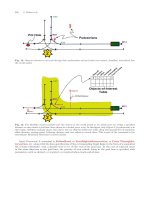
Eye/Head Tracker
In order to avoid having to manually label when the driver was looking away from the simulated road, an
eye/head tracker was used (Fig. 7).
When the driver looked over their shoulder at an image in their blind spot this action caused the eye
tracker to lose eye tracking ability (Fig. 8). This loss sent the eye tracking confidence to a low level. These
periods of low confidence were used as the periods of inattention. This method avoided the need for hand
labeling.
Understanding Driving Activity 53
Table 3. Variables used to detect inattention
Variable Description
steeringWheel Steering wheel angle
accelerator Position of accelerator pedal
distToLeftLaneEdge Perpendicular distance of left front wheel from left lane edge
crossLaneVelocity Rate of change of distToLeftLaneEdge
crossLaneAcceleration Rate of change of crossLaneVelocity
steeringError Difference between steering wheel position and ideal position
for vehicle to travel exactly parallel to lane edges
aheadLaneBearing Angle of road 60 m in front of current vehicle position

Fig. 7. Eye/head tracking during attentive driving
Fig. 8. Loss of eye/head tracking during inattentive driving
6.2 Inattention Data Processing
Data was collected from six different drivers as described above. This data was later synchronized and re-
sampled at a constant sampling rate of 10 Hz. resulting in 40,700 sample vectors. In order to provide more
relevant information to the task at hand, further parameters were derived from the original sensors. These
parameters are as follows:
1. ra9: Running average of the signal over nine previous samples (smoothed version of the signal).
2. rd5: Running difference five samples apart (trend).
3. rv9: Running variance of nine previous samples according to the standard definition of sample variance.
4. ent15: Entropy of the error that a linear predictor makes in trying to predict the signal as described in
[1]. This can be thought of as a measure of randomness or unpredictability of the signal.
5. stat3: Multivariate stationarity of a number of variables simultaneously three samples apart as described
in [27]. Stationarity gives an overall rate of change for a group of signals. Stationarity is one if there are
no changes over the time window and approaches zero for drastic transitions in all signals of the group.
The operations can be combined. For example, “
rd5 ra9” denotes first computing a running difference
five samples apart and then computing the running average over nine samples.
Two different experiments were conducted.
1. The first experiment used only two parameters: steeringWheel and accelerator, and derived seven other
parameters: steeringWheel
rd5 ra9, accelerator rd5 ra9, stat3 of steeringWheel accel,
steeringWheel
ent15 ra9, accelerator ent15 ra9, steeringWheel rv9, and accelerator rv9.
54 K. Torkkola et al.
2. The second experiment used all seven parameters in Table 1 and derived 13 others as follows:
steeringWheel
rd5 ra9, steeringError rd5 ra9, distToLeftLaneEdge rd5 ra9, accelerator rd5 ra9,
aheadLaneBearing
rd5 ra9, stat3 of steeringWheel accel,

stat3
of steeringError crossLaneVelocity distToLeftLaneEdge aheadLaneBearing,
steeringWheel
ent15 ra9, accelerator ent15 ra9, steeringWheel rv9, accelerator rv9,
distToLeftLaneEdge
rv9, and crossLaneVelocity rv9.
Variable Selection for Inattention
In variable selection experiments we are attempting to determine the relative importance of each variable to
the task of inattention detection. First a Random Forest classifier is trained for inattention detection (see
also Sect. 6.2). Variable importances can then be extracted from the trained forest using the approach that
was outlined in Sect. 5.
We present the results in Tables 4 and 5. These tables provide answers to the question “Which sensors
are most important in detecting driver’s inattention?” When just the two basic “driver control” sensors
were used, some new derived variables may provide as much new information as the original signals, namely
the running variance and entropy of steering. When CAS sensors are combined, the situation changes: lane
Table 4. Important sensor signals for inattention detection derived from steering wheel and accelerator pedal
Variable Importance
steeringWheel 100.00
accelerator 87.34
steeringWheel
rv9 68.89
steeringWheel
ent15 ra9 58.44
stat3
of steeringWheel accelerator 41.38
accelerator
ent15 ra9 40.43
accelerator
rv9 35.86
steeringWheel

rd5 ra9 32.59
accelerator
rd5 ra9 29.31
Table 5. Important sensor signals for inattention detection derived from steering wheel, accelerator pedal and CAS
sensors
Variable Importance
distToLeftLaneEdge 100.00
accelerator 87.99
steeringWheel
rv9 73.76
distToLeftLaneEdge
rv9 65.44
distToLeftLaneEdge
rd5 ra9 65.23
steeringWheel 64.54
Stat3
of steeringWheel accel 60.00
steeringWheel
ent15 ra9 57.39
steeringError 57.32
aheadLaneBearing
rd5 ra9 55.33
aheadLeneBearing 51.85
crossLaneVelocity 50.55
Stat3
of steeringError crossLaneVelocity distToLeftLaneEdge aheadLaneBearing 38.07
crossLaneVelocity
rv9 36.50
steeringError
rd5 ra9 33.52

Accelerator
ent15 ra9 29.83
Accelerator
rv9 28.69
steeringWheel
rd5 ra9 27.76
Accelerator
rd5 ra9 20.69
crossLaneAcceleration 20.64
Understanding Driving Activity 55
position (distToLeftLaneEdge) becomes the most important variable together with the accelerator pedal.
Steering wheel variance becomes the most important variable related to steering.
Inattention Detectors
Detection tasks always have a tradeoff between desired recall and precision. Recall denotes the percentage
of total events of interest detected. Precision denotes the percentage of detected events that are true events
of interest and not false detections. A trivial classifier that classifies every instant as a true event would have
100% recall (since none were missed), but its precision would be poor. On the other hand, if the classifier
is so tuned that only events having high certainty are classified as true events, the recall would be low,
missing most of the events, but its precision would be high, since among those that were classified as true
events, only a few would be false detections. Usually any classifier has some means of tuning the threshold of
detection. Where that threshold will be set depends on the demands of the application. It is also noteworthy
to mention that in tasks involving detection of rare events, overall classification accuracy is not a meaningful
measure. In our case only 7.3% of the database was inattention so a trivial classifier classifying everything
as attention would thus have an accuracy of 92.7%. Therefore we will report our results using the recall and
precision statistics for each class.
First, we constructed a Random Forests (RF) classifier of 75 trees using either the driver controls or the
driver controls combined with the CAS sensors. Figure 9 depicts the resulting recall/precision graphs.
One simple figure of merit that allows comparison of two detectors is equal error rate, or equal accuracy,
which denotes the intersection of recall and precision curves. By that figure, basing the inattention detector
only on driver control sensors results in an equal accuracy of 67% for inattention and 97% for attention,

whereas adding CAS sensors raises the accuracies up to 80 and 98%, respectively. For comparison, we used
the same data to train a quadratic classifier [29]. Compared to the RF classifier, the quadratic classifier
performs poorly in this task. We present the results in Table 6 for two different operating points of the
quadratic classifier. The first one (middle rows) is tuned not to make false alarms, but its recall rate remains
low. The second one is compensated for the less frequent occurrences of inattention, but it makes false
alarms about 28% of the time. Random Forest clearly outperforms the quadratic classifier with almost no
false alarms and good recall.
Fig. 9. Precision/recall figures for detection of inattention using only driver controls (left) and driver controls
combined with CAS sensors (right). Random Forest is used as the classifier. Horizontal axis, prior for inattention,
denotes a classifier parameter which can be tuned to produce different precision/recall operating points. This can
be thought of as a weight or cost given to missing inattention events. Typically, if it is desirable not to miss events
(high recall – in this case a high parameter value), the precision may be low – many false detections will be made.
Conversely, if it is desirable not to make false detections (high precision), the recall will be low – not all events will
be detected. Thus, as a figure of merit we use equal accuracy, the operating point where precision equals recall
56 K. Torkkola et al.
Table 6. Comparison of Random Forest (RF) to Quadratic classifier using equal accuracy as the figure of merit
Detector Sensors Inattention (%) Attention (%)
RF Driver control sensors only 67 97
RF Additional CAS sensors 80 98
Quadratic Driver control sensors only 29 91
Quadratic Additional CAS sensors 33 93
Quadratic (prior compensated) Driver control sensors only 58 59
Quadratic (prior compensated) Additional CAS sensors 72 72
Operating point where recall of the desired events equals the precision of the detector
Future Driver Inattention Work
The experiments described in this section are only our first steps in investigating how driver attention can
be detected. We have several ideas of how to improve the accuracy of detectors based on modifications to
our described approach. The first technique will be to treat inattentive periods as longer time segments that
actually have a weighting mechanism that prohibits rapid toggling between states. Also, an edge detector
could be trained to detect the transitions between attention/inattention states instead of states for individual

time samples. Even with improvements we will end up with a less than perfect inattention detector and we
will have to study user experiences in order to define levels of accuracy required before inattention detectors
could be used as an acceptable driver assistant tool.
Future work should also include modeling how drivers “recover” from inattentive periods. Even with
perfect eye tracking it is unlikely that when a driver’s eyes return to the road that the driver is instantly
attentive and aware of his environment. This is a general attention modeling problem and is not specific to
our technique.
Once driver inattention is detected there still needs to be experimentation on how to best assist the
driver. Good driving habits will include periods that we have defined as inattentive, such as a “blind spot”
glance before changing lanes. The system must understand the appropriate frequency and duration of these
“blind spot” glances and not annoy the driver by offering counter-productive or unreasonable advice.
7Conclusion
In this chapter, we have demonstrated three instances of using computational intelligence techniques such
as the random forest method in developing intelligent driver assistance systems. Random Forest appears to
be a very well suited tool for massive heterogeneous data sets that are generated from the driving domain.
A driver activity classifier based on Random Forests is also fast enough to run in real time in a vehicle.
First, the random forest method is used to create a semi-automatic data annotation tool for driving
database creation to support data-driven approaches in the driving domain such as driving state classi-
fication. The tool significantly reduces the manual annotation effort and thus enables the user to verify
automatically generated annotations, rather than annotating from scratch. In experiments going through
the whole database annotation cycle, we have observed sixfold reductions in the annotation time by a
human annotator [25].
Second, the random forest method is employed to identify the sensor variables that are important for
determining the driving maneuvers. Different combinations of sensor variables are identified for different
driving maneuvers. For example, steering wheel angle is important for determining the turning maneuver, and
brake status, acceleration, and headway distance are important for determining the panic brake maneuver.
Third, our random forest technique enabled us to detect driver inattention through the use of sensors
that are available in modern vehicles. We compared both traditional sensors (detecting only steering wheel
angle and accelerator pedal position) and CAS sensors against the performance of a state-of-the-art eye/head
tracker. As expected, the addition of CAS sensors greatly improve the ability for a system to detect inat-

tention. Though not as accurate as eye tracking, a significant percentage of inattentive time samples could
Understanding Driving Activity 57
be detected by monitoring readily available sensors (including CAS sensors) and it is believed that a driver
assistant system could be built to use this information to improve driver attention. The primary advantage
of our system is that it requires only a small amount of code to be added to existing vehicles and avoids the
cost and complexity of adding driver monitors such as eye/head trackers.
A driving simulator is an excellent tool to investigate driver inattention since this allows us to design
experiments and collect data on driver behaviors that may impose a safety risk if these experiments were
performed in a real vehicle. There is still much to be learned about the causes and effects of driver inattention,
but even small steps toward detecting inattention can be helpful in increasing driver performance.
References
1. E.R. Boer. Behavioral entropy as an index of workload. In Proceedings of the IEA/HFES 2000 Congress, pp.
125–128, 2000.
2. E.R. Boer. Behavioral entropy as a measure of driving performance. In Driver Assessment, pp. 225–229, 2001.
3. O. Bousquet and A. Elisseeff. Algorithmic stability and generalization performance. In Proceedings of NIPS, pp.
196–202, 2000.
4. L. Breiman. Bagging predictors. Machine Learning, 24(2):123–140, 1996.
5. L. Breiman. Random forests. Machine Learning, 45(1):5–32, 2001.
6. L. Breiman, J.H. Friedman, R.A. Olshen, and C.J. Stone. Classification and Regression Trees, CRC Press, Boca
Raton, FL, 1984.
7. D. Cohn, L. Atlas, and R. Ladner. Improving generalization with active learning. Machine Learning, 15(2):201–
221, 1994.
8. T.A. Dingus, S.G. Klauer, V.L. Neale, A. Petersen, S.E. Lee, J. Sudweeks, M.A. Perez, J. Hankey, D. Ramsey,
S. Gupta, C. Bucher, Z.R. Doerzaph, J. Jermeland, and R.R. Knipling. The 100 car naturalistic driving study:
Results of the 100-car field experiment performed by Virginia tech transportation institute. Report DOT HS 810
593, National Highway Traffic Safety Administration, Washington DC, April 2006.
9. L. Fletcher, N. Apostoloff, L. Petersson, and A. Zelinsky. Driver assistance systems based on vision in and out of
vehicles. In Proceedings of IEEE Intel ligent Vehicles Symposium, pp. 322–327. IEEE, Piscataway, NJ, June 2003.
10. J. Forbes, T. Huang, K. Kanazawa, and S. Russell. The BATmobile: Towards a Bayesian automated taxi. In
Proceedings of Fourteenth International Joint Conference on Artificial Intel ligence, Montreal, Canada, 1995.

11. I. Guyon and A. Elisseeff. An introduction to feature selection. Journal of Machine Learning Research, 3:1157–
1182, 2003.
12. I. Guyon, S. Gunn, M. Nikravesh, and L. Zadeh. Feature Extraction, Foundations and Applications. Springer,
Berlin Heidelberg New York, 2006.
13. J. Hankey, T.A. Dingus, R.J. Hanowski, W.W. Wierwille, C.A. Monk, and M.J. Moyer. The development of
a design evaluation tool and model of attention demand. Report 5/18/00, National Highway Traffic Safety
Administration, Washington DC, May 18, 2000.
14. R.A. Hess and A. Modjtahedzadeh. A preview control model of driver steering behavior. In Proceedings of IEEE
International Conference on Systems, Man and Cybernetics, pp. 504–509, November 1989.
15. R.A. Hess and A. Modjtahedzadeh. A control theoretic model of driver steering behavior. IEEE Control Systems
Magazine, 10(5):3–8, 1990.
16. H. Liu and H. Motoda. Feature Selection for Knowledge Discovery and Data Mining. Kluwer, Boston, MA, 1998.
17. J.C. McCall and M.M. Trivedi. Driver behavior and situation aware brake assistance for intelligent vehicles.
Proceedings of the IEEE, 95(2):374–387, 2007.
18. V.L. Neale, S.G. Klauer, R.R. Knipling, T.A. Dingus, G.T. Holbrook, and A. Petersen. The 100 car naturalistic
driving study: Phase 1-experimental design. Interim Report DOT HS 809 536, Department of Transportation,
Washington DC, November 2002. Contract No: DTNH22-00-C-07007 by Virginia Tech Transportation Institute.
19. A. Ng, M. Jordan, and Y. Weiss. On spectral clustering: Analysis and an algorithm. In Advances in Neural
Information Processing Systems 14: Proceedings of the NIPS 2001, 2001.
20. N. Oza. Probabilistic models of driver behavior. In Proceedings of Spatial Cognition Conference,Berkeley,CA,
1999.
21. F.J. Pompei, T. Sharon, S.J. Buckley, and J. Kemp. An automobile-integrated system for assessing and reacting
to driver cognitive load. In Proceedings of Convergence 2002, pp. 411–416. IEEE SAE, New York, 2002.
22. L.R. Rabiner. A tutorial on Hidden Markov Models and selected applications in speech recognition. Proceedings
of the IEEE, 77(2):257–286, 1989.
58 K. Torkkola et al.
23. D. Remboski, J. Gardner, D. Wheatley, J. Hurwitz, T. MacTavish, and R.M. Gardner. Driver performance
improvement through the driver advocate: A research initiative toward automotive safety. In Proceedings of the
2000 International Congress on Transportation Electronics, SAE P-360, pp. 509–518, 2000.
24. B. Sch¨olkopf and A. Smola. Learning with Kernels. MIT Press, Cambridge, MA, 2002.

25. C. Schreiner, K. Torkkola, M. Gardner, and K. Zhang. Using machine learning techniques to reduce data anno-
tation time. In Proceedings of the 50th Annual Meeting of the Human Factors and Ergonomics Society,San
Francisco, CA, October 16–20, 2006.
26. P. Smith, M. Shah, and N. da Vitoria Lobo. Adetermining driver visual attention with one camera. IEEE
Transactions on Intelligent Transportation Systems, 4(4):205, 2003.
27. K. Torkkola. Automatic alignment of speech with phonetic transcriptions in real time. In Proceedings of the IEEE
International Conference on Acoustics, Speech and Signal Processing (ICASSP88), pp. 611–614, New York City,
USA, April 11–14, 1988.
28. K. Torkkola, M. Gardner, C. Schreiner, K. Zhang, B. Leivian, and J. Summers. Sensor selection for driving
state recognition. In Proceedings of the World Congress on Computational Intel ligence (WCCI), IJCNN, pp.
9484–9489, Vancouver, Canada, June 16–21, 2006.
29. K. Torkkola, N. Massey, B. Leivian, C. Wood, J. Summers, and S. Kundalkar. Classification of critical driving
events. In Proceedings of the International Conference on Machine Learning and Applications (ICMLA), pp.
81–85, Los Angeles, CA, USA, June 23–24, 2003.
30. K. Torkkola, N. Massey, and C. Wood. Driver inattention detection through intelligent analysis of readily available
sensors. In Proceedings of the 7th Annual IEEE Conference on Intelligent Transportation Systems (ITSC 2004),
pp. 326–331, Washington DC, USA, October 3–6, 2004.
31. K. Torkkola, S. Venkatesan, and H. Liu. Sensor sequence modeling for driving. In Proceedings of the 18th
International FLAIRS Conference, AAAI Press, Clearwater Beach, FL, USA, May 15–17, 2005.
32. W. Van Winsum, M. Martens, and L. Herland. The effects of speech versus tactile driver support messages on
workload, driver behaviour and user acceptance. TNO-report TM-00-C003, TNO, Soesterberg, The Netherlands,
1999.
33. C. Wood, B. Leivian, N. Massey, J. Bieker, and J. Summers. Driver advocate tool. In Driver Assessment, 2001.
Computer Vision and Machine Learning for Enhancing
Pedestrian Safety
Tarak Gandhi and Mohan Manubhai Trivedi
Laboratory for Safe and Intelligent Vehicles (LISA), University of California San Diego, La Jolla, CA 92093, USA,
,
Summary. Accidents involving pedestrians is one of the leading causes of death and injury around the world.
Intelligent driver support systems hold a promise to minimize accidents and save many lives. Such a system would

detect the pedestrian, predict the possibility of collision, and then warn the driver or engage automatic braking or
other safety devices. This chapter describes the framework and issues involved in developing a pedestrian protection
system. It is emphasized that the knowledge of the state of the environment, vehicle, and driver are important for
enhancing safety. Classification, clustering, and machine learning techniques for effectively detecting pedestrians are
discussed, including the application of algorithms such as SVM, Neural Networks, and AdaBoost for the purpose of
distinguishing pedestrians from background. Pedestrians unlike vehicles are capable of sharp turns and speed changes,
therefore their future paths are difficult to predict. In order to estimate the possibility of collision, a probabilistic
framework for pedestrian path prediction is described along with related research. It is noted that sensors in vehicle are
not always sufficient to detect all the pedestrians and other obstacles. Interaction with infrastructure based systems
as well as systems from other vehicles can provide a wide area situational awareness of the scene. Furthermore,
in infrastructure based systems, clustering and learning techniques can be applied to identify typical vehicle and
pedestrian paths and to detect anomalies and potentially dangerous situations. In order to effectively integrate
information from infrastructure and vehicle sources, the importance of developing and standardizing vehicle-vehicle
and vehicle-infrastructure communication systems is also emphasized.
1 Introduction
Intelligent Transportation Systems (ITS) show promise of making road travel safer and comfortable. Auto-
mobile companies have recently taken considerable interest in developing Intelligent Driver Support Systems
(IDSS) for high-end vehicles. These include active cruise control, lane departure warning, blind spot moni-
toring, and pedestrian detection systems based on sensors such as visible light and thermal infrared cameras,
RADARs, or LASER scanners. However, for an effective driver support system, it is desirable to take a
holistic approach, using all available data from the environment, vehicle dynamics, and the driver that can
be obtained using various sensors incorporated in vehicle and infrastructure [35]. Infrastructure based sen-
sors can complement the vehicle sensors by filling gaps and providing more complete information about the
surroundings. Looking in the vehicle at driver’s state is as important as looking out in surroundings in order
to convey warnings to the driver in the most effective and least distracting manner. Furthermore, due to the
highly competitive nature of automobile manufacturing, it is necessary to make such systems cost effective.
This makes multi-functional sensors that are used by several of these systems highly desirable.
Accidents involving pedestrians and other vulnerable road users such as bicyclists are one of the leading
causes of death and injury around the world. In order to reduce these accidents, pedestrian protection
systems need to detect pedestrians, track them over time, and predict the possibility of collision based on

the paths that the pedestrian and the vehicle are likely to take. The system should relay the information
to the driver in efficient and non-distracting manner or to the control system of the vehicle in order to
take preventive actions. Considerable efforts have been made on enhancing pedestrian safety by programs
in United states [3, 4], Europe [2, 5] and Japan [1]. Conferences such as Intelligent Vehicles Symposium [6]
T. Gandhi and M.M. Trivedi: Computer Vision and Machine Learning for Enhancing Pedestrian Safety, Studies in Computational
Intelligence (SCI) 132, 59–77 (2008)
www.springerlink.com
c
 Springer-Verlag Berlin Heidelberg 2008
60 T. Gandhi and M.M. Trivedi
and Intelligent Transportation Systems Conference [7] have a number of publications related to pedestrian
detection every year. The recent survey on pedestrian protection [19] has covered the current research on
pedestrian detection, tracking, and collision prediction. It is observed that detecting pedestrians in cluttered
scenes from a moving vehicle is a challenging problem that involves a number of computational intelligence
techniques spanning image processing, computer vision, pattern recognition, and machine learning. This
paper focuses on specific computational intelligence techniques used in stages of sensor based pedestrian
protection system for detecting and classifying pedestrians, and predicting their trajectories to assess the
possibility of collision.
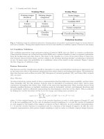
2 Framework for Pedestrian Protection System
Figure 1 shows the components of a general pedestrian protection system. The data from one or more
types of sensors can be processed using computer vision algorithms to detect pedestrians and determine
their trajectories. The trajectories can then be sent to collision prediction module that would predict the
probability of collision between the host vehicle and pedestrians. In the case of high probability of collision,
the driver is given appropriate warning that enables corrective action. If the collision is imminent, the
automatic safety systems could also be triggered to decelerate the vehicle and reduce the impact of collision.
In the following sections we illustrate these components using examples focusing on approaches used for
these tasks.
Pedestrian Detection
Candidate generation
Classification/Verification

Tracking
Environment Sensors in Vehicle and Infrastructure
Imaging sensors: Visible light, near IR, thermal IR
Time of flight sensors: RADARs, LASER scanners
Vehicle
Dynamic
Sensors
Pedestrian
appearance
and motion
models
Collision Prediction
Trajectory prediction
Monte Carlo Simulations
Particle filtering
Pedestrian
behavior
models
Action
Warning driver
Activation of automatic braking,
passive safety systems
Driver State
Sensing
Sensor data
Pedestrian trajectories
Collision probabilities
Fig. 1. Data flow diagram for pedestrian protection systems
Computer Vision and Machine Learning for Enhancing Pedestrian Safety 61
3 Techniques in Pedestrian Detection

Pedestrian detection is usually divided into two stages. The candidate generation stage processes raw data
using simple cues and fast algorithms to identify potential pedestrian candidates. The classification and
verification stage then applies more complex algorithms to the candidates from the attention focusing stage
in order to separate genuine pedestrians from false alarms. However, the line between these stages is often
blurred and some approaches combine the stages into one. Table 1 shows the approaches used by researchers
for stages in pedestrian detection.
3.1 Candidate Generation
Cues such as shape, appearance, motion, and distance can be used to generate potential pedestrian
candidates. Here, we describe selected techniques used for generating pedestrian candidates using these cues.
Chamfer Matching
Chamfer matching is a generic technique to recognize objects based on their shape and appearance using
hierarchical matching with a set of object templates from training images. The original image is converted
to a binary image using an edge detector. A distance transform is then applied to the edge image. Every
pixel r =(x, y) in the distance transformed image has a value d
I
(t) equal to the distance to the nearest edge
pixel:
d
I
(r)= min
r

∈edges(I)
r

− r (1)
The distance transformed image is matched to the binary templates generated from examples. For this
purpose, the template is slided over the image and at every displacement, the chamfer distance between the
image and template is obtained by taking the mean of all the pixels in the distance transform image that
have an ‘on’ pixel in template image:

D(T,I)=
1
|T |

r∈T
d
I
(r)(2)
Positions in the image where the chamfer distance is less than a threshold are considered as successful
matches.
Table 1. Approaches used in stages of pedestrian protection
Publication Candidate generation Feature extraction Classification
Gavrila ECCV00 [20],
IJCV07 [21], Munder
PAMI06 [27 ]
Chamfer matching Image ROI pixels LRF Neural Network
Gandhi MM04 [15],
MVA05 [16]
Omni camera based planar
motion estimation
Gandhi ICIP05 [17],
ITS06 [18]
Stereo based U disparity
analysis
Krotosky IV06 [25] Stereo based U and V
disparity analysis
Histogram of oriented
gradients
Support Vector Machine
Papageorgiou IJCV00 [28] Haar wavelets Support Vector Machine

Dalal CVPR05 [13] Histogram of oriented
gradients
Support Vector Machine
Viola IJCV05 [37] Haar-like features in spatial
and temporal domain
AdaBoost
Park ISI07 [29] Background subtraction,
homography projection
Shape and size of object
62 T. Gandhi and M.M. Trivedi
In order to account for the variations between individual objects, the image is matched with number
of templates. For efficient matching, a template hierarchy is generated using bottom up clustering. All the
training templates are grouped into K clusters, each represented by a prototype template p
k
and the set
of templates S
k
in the cluster. Clustering is performed using using an iterative optimization algorithm that
minimizes an objective function:
E =
K

k=1
max
t
i
∈S
k
D
min

(t
i
,p
k
)(3)
where D
min
(t
i
,p
k
) denotes the minimum chamfer distance between the template t
i
and the prototype p
k
for
all relative displacements between them. The process is repeated recursively by treating the prototypes as
templates and re-clustering them to form a tree as shown in Fig. 2.
For recognition, the given image is recursively matched with the nodes of the template tree, starting
from the root. At any level, the branches where the minimum chamfer distance is greater than a threshold
are pruned to reduce the search time. For remaining nodes, matching is repeated for all children nodes.
Candidates are generated at image positions where the chamfer distance with any of the template nodes is
below threshold.
Motion-Based Detection
Motion is an important cue in detecting pedestrians. In the case of moving platforms, the background
undergoes ego-motion that depends on camera motion as well as the scene structure, which needs to be
accounted for. In [15, 16], a parametric planar motion model is used to describe the ego-motion of the ground
in an omnidirectional camera. The perspective coordinates of a point P on the ground in two consecutive
camera positions is governed by a homography matrix H as:
⎛

⎝
X
b
Y
b
Z
b
⎞
⎠
= λ
⎛
⎝
h
11
h
12
h
13
h
21
h
32
h
33
h
31
h
32
1
⎞

⎠
⎛
⎝
X
a
Y
a
Z
a
⎞
⎠
(4)
The perspective camera coordinates can be mapped to pixel coordinates (u
a
,v
a
)and(u
b
,v
b
)usingthe
internal calibration of the camera:
(u
a
,v
a
)=F
int
([X
a

,Y
a
,Z
a
]
T
),
(u
b
,v
b
)=F
int
([X
b
,Y
b
,Z
b
]
T
)=F
int
(HF
−1
int
(u
a
,v
a

)) (5)
The image motion of the point satisfies the optical flow constraint:
g
u
(u
b
− u
a
)+g
v
(v
b
− v
a
)=−g
t
+ ν (6)
where g
u
, g
v
,andg
t
are the spatial and temporal image gradients and ν is the noise term.
Based on these relations, the parameters of the homography matrix can be estimated using the spatio-
temporal image gradients at every point (u
a
,v
a
) in the first image using non-linear least squares. Based on

these parameters, every point (u
a
,v
a
) on the ground plane in first frame corresponds to a point (u
b
,v
b
)inthe
second frame. Using this transformation, the second image can be transformed to first frame, compensating
the image motion of the ground plane. The objects that have independent motion or height above ground do
not obey the motion model and their motion is not completely compensated. Taking the motion compensated
frame difference between adjacent video frames highlights these areas that are likely to contain pedestrians,
vehicles, or other obstacles. These regions of interest can then be classified using the classification stage.
Figure 3 shows detection of a pedestrian and vehicle from a moving platform. The details of the approach
are described in [15].
Computer Vision and Machine Learning for Enhancing Pedestrian Safety 63
(a) (b) (c) (d)
(e)
Fig. 2. Chamfer matching illustration: (a) template of pedestrian (b) test image (c) edge image (d) distance transform
image (e) template hierarchy (partial) used for matching with distance transform (figure based on [27])
Depth Segmentation Using Binocular Stereo
Binocular stereo imaging can provide useful information about the depth of the objects from the cameras.
This information has been used for disambiguating pedestrians and other objects from features on ground
plane [18, 25, 26], segmenting images based on layers with different depths [14], handling occlusion between
pedestrians [25], and using the size-depth relation to eliminate extraneous objects [32]. For a pair of stereo
cameras with focal length f and baseline distance of B between the cameras situated at the height of H
64 T. Gandhi and M.M. Trivedi
(a)
(b)

(d)
(c)
Fig. 3. Detection of people and vehicles using an omnidirectional camera on a moving platform [15] (a)estimated
motion based on parametric motion of ground plane (b) image pixels used for estimation. Gray pixels are inliers, and
white pixels are outliers. (c) Motion-compensated image difference that captures independently moving objects (d)
detected vehicle and person
above the road as shown in Fig. 4a. An object at distance D will have disparity of d = Bf/D between the
two cameras, that is inversely proportional to object distance. The ground in the same line of sight is farther
away and has a smaller disparity of d
bg
= Bf/D
bg
. Based on this difference, objects having height above
the ground can be separated.
Stereo disparity computation can be performed using software packages such as SRI Stereo Engine [24].
Such software produces a disparity map that gives disparities of individual pixels in the image. In [17],
the concept of U-disparity proposed by Labayrade et al. [26] is used to identify potential obstacles in the
scene using images from a stereo pair of omnidirectional cameras as shown in Fig. 4b. The disparity image
disp(u, v) generated by a stereo engine separates the pedestrian in a layer of nearly constant depth. U-
disparity udisp(u, d) image counts occurrences of every disparity d for each column u in the image. In order
to suppress the ground plane pixels, only the pixels with disparity significantly greater than ground plane
disparity are used.
udisp(u, d)=#{v|disp(u, v)=d, d > d
bg
(u, v)+d
thresh
} (7)
where # stands for number of elements in the set.
Pixels in an object at a particular distance would have nearly same disparity and therefore form a
horizontal ridge in the disparity histogram image. Even if disparities of individual object pixels are inaccurate,

the histogram image clusters the disparities and makes it easier to isolate the objects. Based on the position
of the line segments, the regions containing obstacles can be identified. The nearest (lowest) region with
largest disparity corresponds to the pedestrian. The parts of the virtual view image corresponding to the
U-disparity segments can then be sent to classifier for distinguishing between pedestrians and other objects.
Computer Vision and Machine Learning for Enhancing Pedestrian Safety 65
H
h
0 D D
bg
Cameras
Object
Road
Disparity = d
Disparity = d
bg
B
(a)
(b)
Fig. 4. (a) Stereo geometry (top and side views). The disparity between image positions in the two cameras decrease
with object distance. (b) Stereo based pedestrian candidate generation [17]: Row 1 : Color images from a stereo
pair of omni camera containing pedestrian. Row 2 : Virtual front view images generated from omni images. Row 3 :
Superimposed front view images and disparity image with lighter shades showing nearer objects with larger disparity.
Row 4 : U-disparity image taking histogram of disparities for each column. The lower middle segment in U-disparity
image corresponds to the pedestrian. Other segments corresponds to more distant structures above the ground (figure
based on [17])