A HEAT TRANSFER TEXTBOOK - THIRD EDITION Episode 3 Part 2 potx

514 Chapter 9: Heat transfer in boiling and other phase-change configurations
9.9 Water at 100 atm boils on a nickel heater whose temperature
is 6
◦
C above T
sat
. Find h and q.
9.10 Water boils on a large flat plate at 1 atm. Calculate q
max
if the
plate is operated on the surface of the moon (at
1
6
of g
earth−normal
).
What would q
max
be in a space vehicle experiencing 10
−4
of
g
earth−normal
?
9.11 Water boils on a 0.002 m diameter horizontal copper wire. Plot,
to scale, as much of the boiling curve on log q vs. log ∆T coor-
dinates as you can. The system is at 1 atm.
9.12 Redo Problem 9.11 for a 0.03 m diameter sphere in water at
10 atm.
9.13 Verify eqn. (9.17).
9.14 Make a sketch of the q vs. (T

w
−T
sat
) relation for a pool boiling
process, and invent a graphical method for locating the points
where h is maximum and minimum.
9.15 A 2 mm diameter jet of methanol is directed normal to the
center of a 1.5 cm diameter disk heater at 1 m/s. How many
watts can safely be supplied by the heater?
9.16 Saturated water at 1 atm boils ona½cmdiameter platinum
rod. Estimate the temperature of the rod at burnout.
9.17 Plot (T
w
− T
sat
) and the quality x as a function of position x
for the conditions in Example 9.9. Set x = 0 where x = 0 and
end the plot where the quality reaches 80%.
9.18 Plot (T
w
− T
sat
) and the quality x as a function of position in
an 8 cm I.D. pipe if 0.3kg/s of water at 100
◦
C passes through
it and q
w
= 200, 000 W/m
2

.
9.19 Use dimensional analysis to verify the form of eqn. (9.8).
9.20 Compare the peak heat flux calculated from the data given in
Problem 5.6 with the appropriate prediction. [The prediction
is within 11%.]
Problems 515
9.21 The Kandlikar correlation, eqn. (9.50a), can be adapted sub-
cooled flow boiling, with x = 0 (region B in Fig. 9.19). Noting
that q
w
= h
fb
(T
w
−T
sat
), show that
q
w
=

1058 h
lo
F(Gh
fg
)
−0.7
(T
w
−T

sat
)

1/0.3
in subcooled flow boiling [9.47].
9.22 Verify eqn. (9.53) by repeating the analysis following eqn. (8.47)
but using the b.c. (∂u/∂y)
y=δ
= τ
δ

µ in place of (∂u/∂y)
y=δ
= 0. Verify the statement involving eqn. (9.54).
9.23 A cool-water-carrying pipe 7 cm in outside diameter has an
outside temperature of 40
◦
C. Saturated steam at 80
◦
C flows
across it. Plot
h
condensation
over the range of Reynolds numbers
0  Re
D
 10
6
. Do you get the value at Re
D

= 0 that you would
anticipate from Chapter 8?
9.24 (a) Suppose that you have pits of roughly 0.002 mm diame-
ter in a metallic heater surface. At about what temperature
might you expect water to boil on that surface if the pressure
is 20 atm. (b) Measurements have shown that water at atmo-
spheric pressure can be superheated about 200
◦
C above its
normal boiling point. Roughly how large an embryonic bubble
would be needed to trigger nucleation in water in such a state.
9.25 Obtain the dimensionless functional form of the pool boiling
q
max
equation and the q
max
equation for flow boiling on exter-
nal surfaces, using dimensional analysis.
9.26 A chemist produces a nondegradable additive that will increase
σ by a factor of ten for water at 1 atm. By what factor will the
additive improve q
max
during pool boiling on (a) infinite flat
plates and (b) small horizontal cylinders? By what factor will
it improve burnout in the flow of jet on a disk?
9.27 Steam at 1 atm is blown at 26 m/sovera1cmO.D. cylinder at
90
◦
C. What is h? Can you suggest any physical process within
the cylinder that could sustain this temperature in this flow?

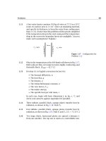
9.28 The water shown in Fig. 9.17 is at 1 atm, and the Nichrome
heater can be approximated as nickel. What is T
w
−T
sat
?
516 Chapter 9: Heat transfer in boiling and other phase-change configurations
9.29 For film boiling on horizontal cylinders, eqn. (9.6) is modified
to
λ
d
= 2π
√
3

g(ρ
f
−ρ
g
)
σ
+
2
(diam.)
2

−1/2
.
If ρ
f

is 748 kg/m
3
for saturated acetone, compare this λ
d
, and
the flat plate value, with Fig. 9.3d.
9.30 Water at 47
◦
C flows through a 13 cm diameter thin-walled tube
at8m/s. Saturated water vapor, at 1 atm, flows across the tube
at 50 m/s. Evaluate T
tube
, U, and q.
9.31 A 1 cm diameter thin-walled tube carries liquid metal through
saturated water at 1 atm. The throughflow of metal is in-
creased until burnout occurs. At that point the metal tem-
perature is 250
◦
C and h inside the tube is 9600 W/m
2
K. What
is the wall temperature at burnout?
9.32 At about what velocity of liquid metal flow does burnout occur
in Problem 9.31 if the metal is mercury?
9.33 Explain, in physical terms, why eqns. (9.23) and (9.24), instead
of differing by a factor of two, are almost equal. How do these
equations change when H

is large?
9.34 A liquid enters the heated section of a pipe at a location z = 0

with a specific enthalpy
ˆ
h
in
. If the wall heat flux is q
w
and the
pipe diameter is D, show that the enthalpy a distance z = L
downstream is
ˆ
h =
ˆ
h
in
+
πD
˙
m

L
0
q
w
dz.
Since the quality may be defined as x ≡ (
ˆ
h −
ˆ
h
f,sat

)

h
fg
, show
that for constant q
w
x =
ˆ
h
in
−
ˆ
h
f,sat
h
fg
+
4q
w
L
GD
9.35 Consider again the x-ray monochrometer described in Problem
7.44. Suppose now that the mass flow rate of liquid nitrogen
is 0.023 kg/s, that the nitrogen is saturated at 110 K when
it enters the heated section, and that the passage horizontal.
Estimate the quality and the wall temperature at end of the
References 517
heated section if F = 4.70 for nitrogen in eqns. (9.50). As
before, assume the silicon to conduct well enough that the heat

load is distributed uniformly over the surface of the passage.
9.36 Use data from Appendix A and Sect. 9.1 to calculate the merit
number, M, for the following potential heat-pipe working flu-
ids over the range 200 K to 600 K in 100 K increments: water,
mercury, methanol, ammonia, and HCFC-22. If data are un-
available for a fluid in some range, indicate so. What fluids are
best suited for particular temperature ranges?
References
[9.1] S. Nukiyama. The maximum and minimum values of the heat q
transmitted from metal to boiling water under atmospheric pres-
sure. J. Jap. Soc. Mech. Eng., 37:367–374, 1934. (transl.: Int. J. Heat
Mass Transfer, vol. 9, 1966, pp. 1419–1433).
[9.2] T. B. Drew and C. Mueller. Boiling. Trans. AIChE, 33:449, 1937.
[9.3] International Association for the Properties of Water and Steam.
Release on surface tension of ordinary water substance. Technical
report, September 1994. Available from the Executive Secretary of
IAPWS or on the internet: />[9.4] J. J. Jasper. The surface tension of pure liquid compounds. J. Phys.
Chem. Ref. Data, 1(4):841–1010, 1972.
[9.5] M. Okado and K. Watanabe. Surface tension correlations for several
fluorocarbon refrigerants. Heat Transfer: Japanese Research,17
(1):35–52, 1988.
[9.6] A. P. Fröba, S. Will, and A. Leipertz. Saturated liquid viscosity and
surface tension of alternative refrigerants. Intl. J. Thermophys.,21
(6):1225–1253, 2000.
[9.7] V.G. Baidakov and I.I. Sulla. Surface tension of propane and isobu-
tane at near-critical temperatures. Russ. J. Phys. Chem., 59(4):551–
554, 1985.
[9.8] P.O. Binney, W G. Dong, and J. H. Lienhard. Use of a cubic equation
to predict surface tension and spinodal limits. J. Heat Transfer,
108(2):405–410, 1986.

518 Chapter 9: Heat transfer in boiling and other phase-change configurations
[9.9] Y. Y. Hsu. On the size range of active nucleation cavities on a
heating surface. J. Heat Transfer, Trans. ASME, Ser. C, 84:207–
216, 1962.
[9.10] G. F. Hewitt. Boiling. In W. M. Rohsenow, J. P. Hartnett, and Y. I.
Cho, editors, Handbook of Heat Transfer, chapter 15. McGraw-Hill,
New York, 3rd edition, 1998.
[9.11] K. Yamagata, F. Hirano, K. Nishiwaka, and H. Matsuoka. Nucleate
boiling of water on the horizontal heating surface. Mem. Fac. Eng.
Kyushu, 15:98, 1955.
[9.12] W. M. Rohsenow. A method of correlating heat transfer data for
surface boiling of liquids. Trans. ASME, 74:969, 1952.
[9.13] I. L. Pioro. Experimental evaluation of constants for the Rohsenow
pool boiling correlation. Int. J. Heat. Mass Transfer, 42:2003–2013,
1999.
[9.14] R. Bellman and R. H. Pennington. Effects of surface tension and
viscosity on Taylor instability. Quart. Appl. Math., 12:151, 1954.
[9.15] V. Sernas. Minimum heat flux in film boiling—a three dimen-
sional model. In Proc. 2nd Can. Cong. Appl. Mech., pages 425–426,
Canada, 1969.
[9.16] H. Lamb. Hydrodynamics. Dover Publications, Inc., New York, 6th
edition, 1945.
[9.17] N. Zuber. Hydrodynamic aspects of boiling heat transfer. AEC
Report AECU-4439, Physics and Mathematics, 1959.
[9.18] J. H. Lienhard and V. K. Dhir. Extended hydrodynamic theory of
the peak and minimum pool boiling heat fluxes. NASA CR-2270,
July 1973.
[9.19] J. H. Lienhard, V. K. Dhir, and D. M. Riherd. Peak pool boiling
heat-flux measurements on finite horizontal flat plates. J. Heat
Transfer, Trans. ASME, Ser. C, 95:477–482, 1973.

[9.20] J. H. Lienhard and V. K. Dhir. Hydrodynamic prediction of peak
pool-boiling heat fluxes from finite bodies. J. Heat Transfer, Trans.
ASME, Ser. C, 95:152–158, 1973.
References 519
[9.21] S. S. Kutateladze. On the transition to film boiling under natural
convection. Kotloturbostroenie, (3):10, 1948.
[9.22] K. H. Sun and J. H. Lienhard. The peak pool boiling heat flux on
horizontal cylinders. Int. J. Heat Mass Transfer, 13:1425–1439,
1970.
[9.23] J. S. Ded and J. H. Lienhard. The peak pool boiling heat flux from
a sphere. AIChE J., 18(2):337–342, 1972.
[9.24] A. L. Bromley. Heat transfer in stable film boiling. Chem. Eng.
Progr., 46:221–227, 1950.
[9.25] P. Sadasivan and J. H. Lienhard. Sensible heat correction in laminar
film boiling and condensation. J. Heat Transfer, Trans. ASME, 109:
545–547, 1987.
[9.26] V. K. Dhir and J. H. Lienhard. Laminar film condensation on plane
and axi-symmetric bodies in non-uniform gravity. J. Heat Transfer,
Trans. ASME, Ser. C, 93(1):97–100, 1971.
[9.27] P. Pitschmann and U. Grigull. Filmverdampfung an waagerechten
zylindern. Wärme- und Stoffübertragung, 3:75–84, 1970.
[9.28] J. E. Leonard, K. H. Sun, and G. E. Dix. Low flow film boiling heat
transfer on vertical surfaces: Part II: Empirical formulations and
application to BWR-LOCA analysis. In Proc. ASME-AIChE Natl. Heat
Transfer Conf. St. Louis, August 1976.
[9.29] J. W. Westwater and B. P. Breen. Effect of diameter of horizontal
tubes on film boiling heat transfer. Chem. Eng. Progr., 58:67–72,
1962.
[9.30] P. J. Berenson. Transition boiling heat transfer from a horizontal
surface. M.I.T. Heat Transfer Lab. Tech. Rep. 17, 1960.

[9.31] J. H. Lienhard and P. T. Y. Wong. The dominant unstable wave-
length and minimum heat flux during film boiling on a horizontal
cylinder. J. Heat Transfer, Trans. ASME, Ser. C, 86:220–226, 1964.
[9.32] L. C. Witte and J. H. Lienhard. On the existence of two transition
boiling curves. Int. J. Heat Mass Transfer, 25:771–779, 1982.
[9.33] J. H. Lienhard and L. C. Witte. An historical review of the hydrody-
namic theory of boiling. Revs. in Chem. Engr., 3(3):187–280, 1985.
520 Chapter 9: Heat transfer in boiling and other phase-change configurations
[9.34] J. R. Ramilison and J. H. Lienhard. Transition boiling heat transfer
and the film transition region. J. Heat Transfer, 109, 1987.
[9.35] J. M. Ramilison, P. Sadasivan, and J. H. Lienhard. Surface factors
influencing burnout on flat heaters. J. Heat Transfer, 114(1):287–
290, 1992.
[9.36] A. E. Bergles and W. M. Rohsenow. The determination of forced-
convection surface-boiling heat transfer. J. Heat Transfer, Trans.
ASME, Series C, 86(3):365–372, 1964.
[9.37] E. J. Davis and G. H. Anderson. The incipience of nucleate boiling
in forced convection flow. AIChE J., 12:774–780, 1966.
[9.38] K. Kheyrandish and J. H. Lienhard. Mechanisms of burnout in sat-
urated and subcooled flow boiling over a horizontal cylinder. In
Proc. ASME–AIChE Nat. Heat Transfer Conf. Denver, Aug. 4–7 1985.
[9.39] A. Sharan and J. H. Lienhard. On predicting burnout in the jet-disk
configuration. J. Heat Transfer, 107:398–401, 1985.
[9.40] A. L. Bromley, N. R. LeRoy, and J. A. Robbers. Heat transfer in
forced convection film boiling. Ind. Eng. Chem., 45(12):2639–2646,
1953.
[9.41] L. C. Witte. Film boiling from a sphere. Ind. Eng. Chem. Funda-
mentals, 7(3):517–518, 1968.
[9.42] L. C. Witte. External flow film boiling. In S. G. Kandlikar, M. Shoji,
and V. K. Dhir, editors, Handbook of Phase Change: Boiling

and Condensation, chapter 13, pages 311–330. Taylor & Francis,
Philadelphia, 1999.
[9.43] J. G. Collier and J. R. Thome. Convective Boiling and Condensation.
Oxford University Press, Oxford, 3rd edition, 1994.
[9.44] J. C. Chen. A correlation for boiling heat transfer to saturated
fluids in convective flow. ASME Prepr. 63-HT-34, 5th ASME-AIChE
Heat Transfer Conf. Boston, August 1963.
[9.45] S. G. Kandlikar. A general correlation for saturated two-phase flow
boiling heat transfer inside horizontal and vertical tubes. J. Heat
Transfer, 112(1):219–228, 1990.
References 521
[9.46] D. Steiner and J. Taborek. Flow boiling heat transfer in vertical
tubes correlated by an asymptotic model. Heat Transfer Engr.,13
(2):43–69, 1992.
[9.47] S. G. Kandlikar and H. Nariai. Flow boiling in circular tubes. In S. G.
Kandlikar, M. Shoji, and V. K. Dhir, editors, Handbook of Phase
Change: Boiling and Condensation, chapter 15, pages 367–402.
Taylor & Francis, Philadelphia, 1999.
[9.48] V. E. Schrock and L. M. Grossman. Forced convection boiling in
tubes. Nucl. Sci. Engr., 12:474–481, 1962.
[9.49] M. M. Shah. Chart correlation for saturated boiling heat transfer:
equations and further study. ASHRAE Trans., 88:182–196, 1982.
[9.50] A. E. Gungor and R. S. H. Winterton. Simplified general correlation
for flow boiling heat transfer inside horizontal and vertical tubes.
Chem. Engr. Res. Des., 65:148–156, 1987.
[9.51] S. G. Kandlikar, S. T. Tian, J. Yu, and S. Koyama. Further assessment
of pool and flow boiling heat transfer with binary mixtures. In
G. P. Celata, P. Di Marco, and R. K. Shah, editors, Two-Phase Flow
Modeling and Experimentation. Edizioni ETS, Pisa, 1999.
[9.52] Y. Taitel and A. E. Dukler. A model for predicting flow regime tran-

sitions in horizontal and near horizontal gas-liquid flows. AIChE
J., 22(1):47–55, 1976.
[9.53] A. E. Dukler and Y. Taitel. Flow pattern transitions in gas–liquid
systems measurement and modelling. In J. M. Delhaye, N. Zuber,
and G. F. Hewitt, editors, Advances in Multi-Phase Flow, volume II.
Hemisphere/McGraw-Hill, New York, 1985.
[9.54] G. F. Hewitt. Burnout. In G. Hetsroni, editor, Handbook of Multi-
phase Systems, chapter 6, pages 66–141. McGraw-Hill, New York,
1982.
[9.55] Y. Katto. A generalized correlation of critical heat flux for
the forced convection boiling in vertical uniformly heated round
tubes. Int. J. Heat Mass Transfer, 21:1527–1542, 1978.
[9.56] Y. Katto and H. Ohne. An improved version of the generalized
correlation of critical heat flux for convective boiling in uniformly
522 Chapter 9: Heat transfer in boiling and other phase-change configurations
heated vertical tubes. Int. J. Heat. Mass Transfer, 27(9):1641–1648,
1984.
[9.57] P. B. Whalley. Boiling, Condensation, and Gas-Liquid Flow. Oxford
University Press, Oxford, 1987.
[9.58] B. Chexal, J. Horowitz, G. McCarthy, M. Merilo, J P. Sursock, J. Har-
rison, C. Peterson, J. Shatford, D. Hughes, M. Ghiaasiaan, V.K. Dhir,
W. Kastner, and W. Köhler. Two-phase pressure drop technology
for design and analysis. Tech. Rept. 113189, Electric Power Re-
search Institute, Palo Alto, CA, August 1999.
[9.59] I. G. Shekriladze and V. I. Gomelauri. Theoretical study of laminar
film condensation of flowing vapour. Int. J. Heat. Mass Transfer,
9:581–591, 1966.
[9.60] P. J. Marto. Condensation. In W. M. Rohsenow, J. P. Hartnett, and
Y. I. Cho, editors, Handbook of Heat Transfer, chapter 14. McGraw-
Hill, New York, 3rd edition, 1998.

[9.61] J. Rose, Y. Utaka, and I. Tanasawa. Dropwise condensation. In S. G.
Kandlikar, M. Shoji, and V. K. Dhir, editors, Handbook of Phase
Change: Boiling and Condensation, chapter 20. Taylor & Francis,
Philadelphia, 1999.
[9.62] D. W. Woodruff and J. W. Westwater. Steam condensation on elec-
troplated gold: effect of plating thickness. Int. J. Heat. Mass Trans-
fer, 22:629–632, 1979.
[9.63] P. D. Dunn and D. A. Reay. Heat Pipes. Pergamon Press Ltd., Oxford,
UK, 4th edition, 1994.
Part IV
Thermal Radiation Heat Transfer
523

10. Radiative heat transfer
The sun that shines from Heaven shines but warm,
And, lo, I lie between that sun and thee:
The heat I have from thence doth little harm,
Thine eye darts forth the fire that burneth me:
And were I not immortal, life were done
Between this heavenly and earthly sun.
Venus and Adonis, Wm. Shakespeare, 1593
10.1 The problem of radiative exchange
Chapter 1 described the elementary mechanisms of heat radiation. Be-
fore we proceed, you should reflect upon what you remember about the
following key ideas from Chapter 1:
• Electromagnetic wave spectrum • The Stefan-Boltzmann law
• Heat radiation & infrared radiation • Wien’s law & Planck’s law
• Black body • Radiant heat exchange
• Absorptance, α • Configuration factor, F
1–2

• Reflectance, ρ • Emittance, ε
• Transmittance, τ • Transfer factor, F
1–2
• α + ρ +τ = 1 • Radiation shielding
• e(T) and e
λ
(T ) for black bodies
The additional concept of a radiation heat transfer coefficient was devel-
oped in Section 2.3. We presume that all these concepts are understood.
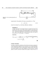
The heat exchange problem
Figure 10.1 shows two arbitrary surfaces radiating energy to one another.
The net heat exchange, Q
net
, from the hotter surface (1) to the cooler
525
526 Radiative heat transfer §10.1
Figure 10.1 Thermal radiation between two arbitrary surfaces.
surface (2) depends on the following influences:
• T
1
and T
2
.
• The areas of (1) and (2), A
1
and A
2
.
• The shape, orientation, and spacing of (1) and (2).
• The radiative properties of the surfaces.

• Additional surfaces in the environment, whose radiation may be
reflected by one surface to the other.
• The medium between (1) and (2) if it absorbs, emits, or “reflects”
radiation. (When the medium is air, we can usually neglect these
effects.)
If surfaces (1) and (2) are black, if they are surrounded by air, and if
no heat flows between them by conduction or convection, then only the
§10.1 The problem of radiative exchange 527
first three considerations are involved in determining Q
net
. We saw some
elementary examples of how this could be done in Chapter 1, leading to
Q
net
= A
1
F
1–2
σ

T
4
1
−T
4
2

(10.1)
The last three considerations complicate the problem considerably. In
Chapter 1, we saw that these nonideal factors are sometimes included in

a transfer factor F
1–2
, such that
Q
net
= A
1
F
1–2
σ

T
4
1
−T
4
2

(10.2)
Before we undertake the problem of evaluating heat exchange among real
bodies, we need several definitions.
Some definitions
Emittance. A real body at temperature T does not emit with the black
body emissive power e
b
= σT
4
but rather with some fraction, ε,ofe
b
.

The same is true of the monochromatic emissive power, e
λ
(T ), which is
always lower for a real body than the black body value given by Planck’s
law, eqn. (1.30). Thus, we define either the monochromatic emittance, ε
λ
:
ε
λ
≡
e
λ
(
λ, T
)
e
λ
b
(
λ, T
)
(10.3)
or the total emittance, ε:
ε ≡
e(T)
e
b
(T )
=


∞
0
e
λ
(
λ, T
)
dλ
σT
4
=

∞
0
ε
λ
e
λ
b
(
λ, T
)
dλ
σT
4
(10.4)
For real bodies, both ε and ε
λ
are greater than zero and less than one;
for black bodies, ε = ε

λ
= 1. The emittance is determined entirely by the
properties of the surface of the particular body and its temperature. It
is independent of the environment of the body.
Table 10.1 lists typical values of the total emittance for a variety of
substances. Notice that most metals have quite low emittances, unless
they are oxidized. Most nonmetals have emittances that are quite high—
approaching the black body limit of unity.
One particular kind of surface behavior is that for which ε
λ
is indepen-
dent of λ. We call such a surface a gray body. The monochromatic emis-
sive power, e
λ
(T ), for a gray body is a constant fraction, ε,ofe
b
λ
(T ),as
indicated in the inset of Fig. 10.2. In other words, for a gray body, ε
λ
= ε.
Table 10.1 Total emittances for a variety of surfaces [10.1]
Metals Nonmetals
Surface Temp. (
◦
C) ε Surface Temp. (
◦
C) ε
Aluminum Asbestos 40 0.93–0.97
Polished, 98% pure 200−600 0.04–0.06 Brick

Commercial sheet 90 0.09 Red, rough 40 0.93
Heavily oxidized 90−540 0.20–0.33 Silica 980 0.80–0.85
Brass Fireclay 980 0.75
Highly polished 260 0.03 Ordinary refractory 1090 0.59
Dull plate 40−260 0.22 Magnesite refractory 980 0.38
Oxidized 40−260 0.46–0.56 White refractory 1090 0.29
Copper Carbon
Highly polished electrolytic 90 0.02 Filament 1040−1430 0.53
Slightly polished to dull 40 0.12–0.15 Lampsoot 40 0.95
Black oxidized 40 0.76 Concrete, rough 40 0.94
Gold: pure, polished 90−600 0.02–0.035 Glass
Iron and steel Smooth 40 0.94
Mild steel, polished 150−480 0.14–0.32 Quartz glass (2 mm) 260−540 0.96–0.66
Steel, polished 40−260 0.07–0.10 Pyrex 260−540 0.94–0.74
Sheet steel, rolled 40 0.66 Gypsum 40 0.80–0.90
Sheet steel, strong 40 0.80 Ice 0 0.97–0.98
rough oxide
Cast iron, oxidized 40−260 0.57–0.66 Limestone 400−260 0.95–0.83
Iron, rusted 40 0.61–0.85 Marble 40 0.93–0.95
Wrought iron, smooth 40 0.35 Mica 40 0.75
Wrought iron, dull oxidized 20−360 0.94 Paints
Stainless, polished 40 0.07–0.17 Black gloss 40 0.90
Stainless, after repeated 230−900 0.50–0.70 White paint 40 0.89–0.97
heating Lacquer 40 0.80–0.95
Lead Various oil paints 40 0.92–0.96
Polished 40−260 0.05–0.08 Red lead 90 0.93
Oxidized 40−200 0.63 Paper
Mercury: pure, clean 40−90 0.10–0.12 White 40 0.95–0.98
Platinum Other colors 40 0.92–0.94
Pure, polished plate 200−590 0.05–0.10 Roofing 40 0.91

Oxidized at 590
◦
C 260−590 0.07–0.11 Plaster, rough lime 40−260 0.92
Drawn wire and strips 40−1370 0.04–0.19 Quartz 100−1000 0.89–0.58
Silver 200 0.01–0.04 Rubber 40 0.86–0.94
Tin 40−90 0.05 Snow 10−20 0.82
Tungsten Water, thickness ≥0.1 mm 40 0.96
Filament 540−1090 0.11–0.16 Wood 40 0.80–0.90
Filament 2760 0.39 Oak, planed 20 0.90
528
§10.1 The problem of radiative exchange 529
Figure 10.2 Comparison of the sun’s energy as typically seen
through the earth’s atmosphere with that of a black body hav-
ing the same mean temperature, size, and distance from the
earth. (Notice that e
λ
, just outside the earth’s atmosphere, is
far less than on the surface of the sun because the radiation
has spread out over a much greater area.)
No real body is gray, but many exhibit approximately gray behavior. We
see in Fig. 10.2, for example, that the sun appears to us on earth as an
approximately gray body with an emittance of approximately 0.6. Some
materials—for example, copper, aluminum oxide, and certain paints—are
actually pretty close to being gray surfaces at normal temperatures.
Yet the emittance of most common materials and coatings varies with
wavelength in the thermal range. The total emittance accounts for this
behavior at a particular temperature. By using it, we can write the emis-
sive power as if the body were gray, without integrating over wavelength:
e(T) = εσT
4

(10.5)
We shall use this type of “gray body approximation” often in this chapter.
530 Radiative heat transfer §10.1
Specular or mirror-like
reflection of incoming ray.
Reflection which is
between diffuse and
specular (a real surface).
Diffuse radiation in which
directions of departure are
uninfluenced by incoming
ray angle, θ.
Figure 10.3 Specular and diffuse reflection of radiation.
(Arrows indicate magnitude of the heat flux in the directions
indicated.)
In situations where surfaces at very different temperatures are in-
volved, the wavelength dependence of ε
λ
must be dealt with explicitly.
This occurs, for example, when sunlight heats objects here on earth. So-
lar radiation (from a high temperature source) is on visible wavelengths,
whereas radiation from low temperature objects on earth is mainly in the
infrared range. We look at this issue further in the next section.
Diffuse and specular emittance and reflection. The energy emitted by
a non-black surface, together with that portion of an incoming ray of
energy that is reflected by the surface, may leave the body diffusely or
specularly, as shown in Fig. 10.3. That energy may also be emitted or
reflected in a way that lies between these limits. A mirror reflects visible
radiation in an almost perfectly specular fashion. (The “reflection” of a
billiard ball as it rebounds from the side of a pool table is also specular.)

When reflection or emission is diffuse, there is no preferred direction for
outgoing rays. Black body emission is always diffuse.
The character of the emittance or reflectance of a surface will nor-
mally change with the wavelength of the radiation. If we take account of
both directional and spectral characteristics, then properties like emit-
tance and reflectance depend on wavelength, temperature, and angles
of incidence and/or departure. In this chapter, we shall assume diffuse
§10.1 The problem of radiative exchange 531
behavior for most surfaces. This approximation works well for many
problems in engineering, in part because most tabulated spectral and to-
tal emittances have been averaged over all angles (in which case they are
properly called hemispherical properties).
Experiment 10.1
Obtain a flashlight with as narrow a spot focus as you can find. Direct
it at an angle onto a mirror, onto the surface of a bowl filled with sugar,
and onto a variety of other surfaces, all in a darkened room. In each case,
move the palm of your hand around the surface of an imaginary hemi-
sphere centered on the point where the spot touches the surface. Notice
how your palm is illuminated, and categorize the kind of reflectance of
each surface—at least in the range of visible wavelengths.
Intensity of radiation. To account for the effects of geometry on radi-
ant exchange, we must think about how angles of orientation affect the
radiation between surfaces. Consider radiation from a circular surface
element, dA, as shown at the top of Fig. 10.4. If the element is black,
the radiation that it emits is indistinguishable from that which would be
emitted from a black cavity at the same temperature, and that radiation
is diffuse — the same in all directions. If it were non-black but diffuse,
the heat flux leaving the surface would again be independent of direc-
tion. Thus, the rate at which energy is emitted in any direction from this
diffuse element is proportional to the projected area of dA normal to the

direction of view, as shown in the upper right side of Fig. 10.4.
If an aperture of area dA
a
is placed at a radius r and angle θ from
dA and is normal to the radius, it will see dA as having an area cos θdA.
The energy dA
a
receives will depend on the solid angle,
1
dω, it sub-
tends. Radiation that leaves dA within the solid angle dω stays within
dω as it travels to dA
a
. Hence, we define a quantity called the intensity
of radiation, i (W/m
2
·steradian) using an energy conservation statement:
dQ
outgoing
= (i dω)(cos θ dA) =

radiant energy from dA
that is intercepted by dA
a
(10.6)
1
The unit of solid angle is the steradian. One steradian is the solid angle subtended
by a spherical segment whose area equals the square of its radius. A full sphere there-
fore subtends 4πr
2

/r
2
= 4π steradians. The aperture dA
a
subtends dω = dA
a

r
2
.
532 Radiative heat transfer §10.1
Figure 10.4 Radiation intensity through a unit sphere.
Notice that while the heat flux from dA decreases with θ (as indicated
on the right side of Fig. 10.4), the intensity of radiation from a diffuse
surface is uniform in all directions.
Finally, we compute i in terms of the heat flux from dA by dividing
eqn. (10.6)bydA and integrating over the entire hemisphere. For conve-
nience we set r = 1, and we note (see Fig. 10.4) that dω = sin θdθdφ.
q
outgoing
=

2π
φ=0

π/2
θ=0
i cosθ
(
sin θdθdφ

)
= πi (10.7a)
§10.2 Kirchhoff’s law 533
In the particular case of a black body,
i
b
=
e
b
π
=
σT
4
π
= fn
(
T only
)
(10.7b)
For a given wavelength, we likewise define the monochromatic intensity
i
λ
=
e
λ
π
= fn
(
T,λ
)

(10.7c)
10.2 Kirchhoff’s law
The problem of predicting α
The total emittance, ε, of a surface is determined only by the phys-
ical properties and temperature of that surface, as can be seen from
eqn. (10.4). The total absorptance, α, on the other hand, depends on
the source from which the surface absorbs radiation, as well as the sur-
face’s own characteristics. This happens because the surface may absorb
some wavelengths better than others. Thus, the total absorptance will
depend on the way that incoming radiation is distributed in wavelength.
And that distribution, in turn, depends on the temperature and physical
properties of the surface or surfaces from which radiation is absorbed.
The total absorptance α thus depends on the physical properties and
temperatures of all bodies involved in the heat exchange process. Kirch-
hoff’s law
2
is an expression that allows α to be determined under certain
restrictions.
Kirchhoff’s law
Kirchhoff’s law is a relationship between the monochromatic, directional
emittance and the monochromatic, directional absorptance for a surface
that is in thermodynamic equilibrium with its surroundings
ε
λ
(
T,θ,φ
)
= α
λ
(

T,θ,φ
)
exact form of
Kirchhoff’s law
(10.8a)
Kirchhoff’s law states that a body in thermodynamic equilibrium emits
as much energy as it absorbs in each direction and at each wavelength. If
2
Gustav Robert Kirchhoff (1824–1887) developed important new ideas in electrical
circuit theory, thermal physics, spectroscopy, and astronomy. He formulated this par-
ticular “Kirchhoff’s Law” when he was only 25. He and Robert Bunsen (inventor of the
Bunsen burner) subsequently went on to do significant work on radiation from gases.
534 Radiative heat transfer §10.2
this were not so, for example, a body might absorb more energy than it
emits in one direction, θ
1
, and might also emit more than it absorbs in an-
other direction, θ
2
. The body would thus pump heat out of its surround-
ings from the first direction, θ
1
, and into its surroundings in the second
direction, θ
2
. Since whatever matter lies in the first direction would be
refrigerated without any work input, the Second Law of Thermodynam-
ics would be violated. Similar arguments can be built for the wavelength
dependence. In essence, then, Kirchhoff’s law is a consequence of the
laws of thermodynamics.

For a diffuse body, the emittance and absorptance do not depend on
the angles, and Kirchhoff’s law becomes
ε
λ
(
T
)
= α
λ
(
T
)
diffuse form of
Kirchhoff’s law
(10.8b)
If, in addition, the body is gray, Kirchhoff’s law is further simplified
ε
(
T
)
= α
(
T
)
diffuse, gray form
of Kirchhoff’s law
(10.8c)
Equation (10.8c) is the most widely used form of Kirchhoff’s law. Yet, it
is a somewhat dangerous result, since many surfaces are not even ap-
proximately gray. If radiation is emitted on wavelengths much different

from those that are absorbed, then a non-gray surface’s variation of ε
λ
and α
λ
with wavelength will matter, as we discuss next.
Total absorptance during radiant exchange
Let us restrict our attention to diffuse surfaces, so that eqn. (10.8b)is
the appropriate form of Kirchhoff’s law. Consider two plates as shown
in Fig. 10.5. Let the plate at T
1
be non-black and that at T
2
be black. Then
net heat transfer from plate 1 to plate 2 is the difference between what
plate 1 emits and what it absorbs. Since all the radiation reaching plate
1 comes from a black source at T
2
, we may write
q
net
=

∞
0
ε
λ
1
(T
1
)e

λ
b
(T
1
)dλ

 
emitted by plate 1
−

∞
0
α
λ
1
(T
1
)e
λ
b
(T
2
)dλ

 
radiation from plate 2
absorbed by plate 1
(10.9)
From eqn. (10.4), we may write the first integral in terms of total emit-
tance, as ε

1
σT
4
1
.Wedefine the total absorptance, α
1
(T
1
,T
2
), as the sec-
§10.2 Kirchhoff’s law 535
Figure 10.5 Heat transfer between two
infinite parallel plates.
ond integral divided by σT
4
2
. Hence,
q
net
= ε
1
(T
1
)σ T
4
1
  
emitted by plate 1
− α

1
(T
1
,T
2
)σ T
4
2
  
absorbed by plate 1
(10.10)
We see that the total absorptance depends on T
2
, as well as T
1
.
Why does total absorptance depend on both temperatures? The de-
pendence on T
1
is simply because α
λ
1
is a property of plate 1 that may
be temperature dependent. The dependence on T
2
is because the spec-
trum of radiation from plate 2 depends on the temperature of plate 2
according to Planck’s law, as was shown in Fig. 1.15.
As a typical example, consider solar radiation incident on a warm
roof, painted black. From Table 10.1, we see that ε is on the order of

0.94. It turns out that α is just about the same. If we repaint the roof
white, ε will not change noticeably. However, much of the energy ar-
riving from the sun is carried in visible wavelengths, owing to the sun’s
very high temperature (about 5800 K).
3
Our eyes tell us that white paint
reflects sunlight very strongly in these wavelengths, and indeed this is
the case — 80 to 90% of the sunlight is reflected. The absorptance of
3
Ninety percent of the sun’s energy is on wavelengths between 0.33 and 2.2 µm (see
Figure 10.2). For a black object at 300 K, 90% of the radiant energy is between 6.3 and
42 µm, in the infrared.
536 Radiative heat transfer §10.3
white paint to energy from the sun is only 0.1 to 0.2 — much less than
ε for the energy it emits, which is mainly at infrared wavelengths. For
both paints, eqn. (10.8b) applies. However, in this situation, eqn. (10.8c)
is only accurate for the black paint.
The gray body approximation
Let us consider our facing plates again. If plate 1 is painted with white
paint, and plate 2 is at a temperature near plate 1 (say T
1
= 400 K and
T
2
= 300 K, to be specific), then the incoming radiation from plate 2 has
a wavelength distribution not too dissimilar to plate 1. We might be very
comfortable approximating ε
1
 α
1

. The net heat flux between the plates
can be expressed very simply
q
net
= ε
1
σT
4
1
−α
1
(T
1
,T
2
)σ T
4
2
 ε
1
σT
4
1
−ε
1
σT
4
2
= ε
1

σ

T
4
1
−T
4
2

(10.11)
In effect, we are approximating plate 1 as a gray body.
In general, the simplest first estimate for total absorptance is the dif-
fuse, gray body approximation, eqn. (10.8c). It will be accurate either if
the monochromatic emittance does not vary strongly with wavelength or
if the bodies exchanging radiation are at similar absolute temperatures.
More advanced texts describe techniques for calculating total absorp-
tance (by integration) in other situations [10.2, 10.3].
One situation in which eqn. (10.8c) should always be mistrusted is
when solar radiation is absorbed by a low temperature object — a space
vehicle or something on earth’s surface, say. In this case, the best first ap-
proximation is to set total absorptance to a value for visible wavelengths
of radiation (near 0.5 µm). Total emittance may be taken at the object’s
actual temperature, typically for infrared wavelengths. We return to solar
absorptance in Section 10.6.
10.3 Radiant heat exchange between two finite
black bodies
Let us now return to the purely geometric problem of evaluating the view
factor, F
1–2
. Although the evaluation of F

1–2
is also used in the calculation
§10.3 Radiant heat exchange between two finite black bodies 537
Figure 10.6 Some configurations for which the value of the
view factor is immediately apparent.
of heat exchange among diffuse, nonblack bodies, it is the only correction
of the Stefan-Boltzmann law that we need for black bodies.
Some evident results. Figure 10.6 shows three elementary situations in
which the value of F
1–2
is evident using just the definition:
F
1–2
≡ fraction of field of view of (1) occupied by (2).
When the surfaces are each isothermal and diffuse, this corresponds to
F
1–2
= fraction of energy leaving (1) that reaches (2)
A second apparent result in regard to the view factor is that all the
energy leaving a body (1) reaches something else. Thus, conservation of
energy requires
1 = F
1–1
+F
1–2
+F
1–3
+···+F
1–n
(10.12)

where (2), (3),…,(n) are all of the bodies in the neighborhood of (1).
Figure 10.7 shows a representative situation in which a body (1) is sur-
rounded by three other bodies. It sees all three bodies, but it also views
538 Radiative heat transfer §10.3
Figure 10.7 A body (1) that views three other bodies and itself
as well.
itself, in part. This accounts for the inclusion of the view factor, F
1–1
in
eqn. (10.12).
By the same token, it should also be apparent from Fig. 10.7 that the
kind of sum expressed by eqn. (10.12) would also be true for any subset
of the bodies seen by surface 1. Thus,
F
1–(2+3)
= F
1–2
+F
1–3
Of course, such a sum makes sense only when all the view factors are
based on the same viewing surface (surface 1 in this case). One might be
tempted to write this sort of sum in the opposite direction, but it would
clearly be untrue,
F
(2+3)–1
≠ F
2–1
+F
3–1
,

since each view factor is for a different viewing surface—(2 + 3),2,and
3, in this case.
View factor reciprocity. So far, we have referred to the net radiation
from black surface (1) to black surface (2) as Q
net
. Let us refine our
notation a bit, and call this Q
net
1–2
:
Q
net
1–2
= A
1
F
1–2
σ

T
4
1
−T
4
2

(10.13)
Likewise, the net radiation from (2) to (1) is
Q
net

2–1
= A
2
F
2–1
σ

T
4
2
−T
4
1

(10.14)