A HEAT TRANSFER TEXTBOOK - THIRD EDITION Episode 3 Part 3 doc

§10.3 Radiant heat exchange between two finite black bodies 539
Of course, Q
net
1–2
=−Q
net
2–1
. It follows that
A
1
F
1–2
σ

T
4
1
−T
4
2

=−A
2
F
2–1
σ

T
4
2
−T

4
1

or
A
1
F
1–2
= A
2
F
2–1
(10.15)
This result, called view factor reciprocity, is very useful in calculations.
Example 10.1
A jet of liquid metal at 2000
◦
C pours from a crucible. It is 3 mm in di-
ameter. A long cylindrical radiation shield, 5 cm diameter, surrounds
the jet through an angle of 330
◦
, but there is a 30
◦
slit in it. The jet
and the shield radiate as black bodies. They sit in a room at 30
◦
C, and
the shield has a temperature of 700
◦
C. Calculate the net heat transfer:

from the jet to the room through the slit; from the jet to the shield;
and from the inside of the shield to the room.
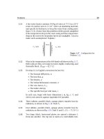
Solution. By inspection, we see that F
jet–room
= 30/360 = 0.08333
and F
jet–shield
= 330/360 = 0.9167. Thus,
Q
net
jet–room
= A
jet
F
jet–room
σ

T
4
jet
−T
4
room

=

π(0.003) m
2
m length


(0.08333)(5.67 ×10
−8
)

2273
4
−303
4

= 1, 188 W/m
Likewise,
Q
net
jet–shield
= A
jet
F
jet–shield
σ

T
4
jet
−T
4
shield

=

π(0.003) m

2
m length

(0.9167)(5.67 ×10
−8
)

2273
4
−973
4

= 12, 637 W/m
The heat absorbed by the shield leaves it by radiation and convection
to the room. (A balance of these effects can be used to calculate the
shield temperature given here.)
To find the radiation from the inside of the shield to the room, we
need F
shield–room
. Since any radiation passing out of the slit goes to the
540 Radiative heat transfer §10.3
room, we can find this view factor equating view factors to the room
with view factors to the slit. The slit’s area is A
slit
= π(0.05)30/360 =
0.01309 m
2
/m length. Hence, using our reciprocity and summation
rules, eqns. (10.12) and (10.15),
F

slit–jet
=
A
jet
A
slit
F
jet–room
=
π(0.003)
0.01309
(0.0833) = 0.0600
F
slit–shield
= 1 −F
slit–jet
−F
slit–slit
  
0
= 1 −0.0600 −0 = 0.940
F
shield–room
=
A
slit
A
shield
F
slit–shield

=
0.01309
π(0.05)(330)/(360)
(0.940) = 0.08545
Hence, for heat transfer from the inside of the shield only,
Q
net
shield–room
= A
shield
F
shield–room
σ

T
4
shield
−T
4
room

=

π(0.05)330
360

(0.08545)(5.67 ×10
−8
)


973
4
−303
4

= 619 W/m
Both the jet and the inside of the shield have relatively small view
factors to the room, so that comparatively little heat is lost through
the slit.
Calculation of the black-body view factor, F
1–2
. Consider two elements,
dA
1
and dA
2
, of larger black bodies (1) and (2), as shown in Fig. 10.8.
Body (1) and body (2) are each isothermal. Since element dA
2
subtends
a solid angle dω
1
, we use eqn. (10.6) to write
dQ
1to2
= (i
1
dω
1
)(cos β

1
dA
1
)
But from eqn. (10.7b),
i
1
=
σT
4
1
π
Note that because black bodies radiate diffusely, i
1
does not vary with
angle; and because these bodies are isothermal, it does not vary with
position. The element of solid angle is given by
dω
1
=
cos β
2
dA
2
s
2
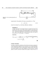
§10.3 Radiant heat exchange between two finite black bodies 541
Figure 10.8 Radiant exchange between two black elements
that are part of the bodies (1) and (2).
where s is the distance from (1) to (2) and cos β

2
enters because dA
2
is
not necessarily normal to s. Thus,
dQ
1to2
=
σT
4
1
π

cos β
1
cos β
2
dA
1
dA
2
s
2

By the same token,
dQ
2to1
=
σT
4

2
π

cos β
2
cos β
1
dA
2
dA
1
s
2

Then
Q
net
1–2
= σ

T
4
1
−T
4
2


A
1


A
2
cos β
1
cos β
2
πs
2
dA
1
dA
2
(10.16)
The view factors F
1–2
and F
2–1
are immediately obtainable from eqn.
(10.16). If we compare this result with Q
net
1–2
= A
1
F
1–2
σ(T
4
1
− T

4
2
),we
get
F
1–2
=
1
A
1

A
1

A
2
cos β
1
cos β
2
πs
2
dA
1
dA
2
(10.17a)
542 Radiative heat transfer §10.3
From the inherent symmetry of the problem, we can also write
F

2–1
=
1
A
2

A
2

A
1
cos β
2
cos β
1
πs
2
dA
2
dA
1
(10.17b)
You can easily see that eqns. (10.17a) and (10.17b) are consistent with
the reciprocity relation, eqn. (10.15).
The direct evaluation of F
1–2
from eqn. (10.17a) becomes fairly in-
volved, even for the simplest configurations. Siegel and Howell [10.4]
provide a comprehensive discussion of such calculations and a large cat-
alog of their results. Howell [10.5] gives an even more extensive tabula-

tion of view factor equations, which is now available on the World Wide
Web. At present, no other reference is as complete.
We list some typical expressions for view factors in Tables 10.2 and
10.3. Table 10.2 gives calculated values of F
1–2
for two-dimensional
bodies—various configurations of cylinders and strips that approach in-
finite length. Table 10.3 gives F
1–2
for some three-dimensional configu-
rations.
Many view factors have been evaluated numerically and presented
in graphical form for easy reference. Figure 10.9, for example, includes
graphs for configurations 1, 2, and 3 from Table 10.3. The reader should
study these results and be sure that the trends they show make sense.
Is it clear, for example, that F
1–2
→ constant, which is < 1 in each case,
as the abscissa becomes large? Can you locate the configuration on the
right-hand side of Fig. 10.6 in Fig. 10.9? And so forth.
Figure 10.10 shows view factors for another kind of configuration—
one in which one area is very small in comparison with the other one.
Many solutions like this exist because they are a bit less difficult to cal-
culate, and they can often be very useful in practice.
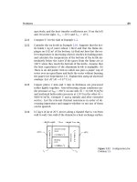
Example 10.2
A heater (h) as shown in Fig. 10.11 radiates to the partially conical
shield (s) that surrounds it. If the heater and shield are black, calcu-
late the net heat transfer from the heater to the shield.
Solution. First imagine a plane (i) laid across the open top of the
shield:

F
h−s
+F
h−i
= 1
But F
h−i
can be obtained from Fig. 10.9 or case 3 of Table 10.3,
Table 10.2 View factors for a variety of two-dimensional con-
figurations (infinite in extent normal to the paper)
Configuration Equation
1.
F
1–2
= F
2–1
=

1 +

h
w

2
−

h
w

2.

F
1–2
= F
2–1
= 1 − sin(α/2)
3.
F
1–2
=
1
2


1 +
h
w
−

1 +

h
w

2


4.
F
1–2
= (A

1
+A
2
−A
3
)

2A
1
5.
F
1–2
=
r
b − a

tan
−1
b
c
−tan
−1
a
c

6.
Let X = 1 +s/D. Then:
F
1–2
= F

2–1
=
1
π


X
2
−1 + sin
−1
1
X
−X

7.
F
1–2
= 1,F
2–1
=
r
1
r
2
, and
F
2–2
= 1 − F
2–1
= 1 −

r
1
r
2
543
Table 10.3 View factors for some three-dimensional configurations
Configuration Equation
1.
Let X = a/c and Y = b/c. Then:
F
1–2
=
2
πXY



ln

(1 +X
2
)(1 +Y
2
)
1 +X
2
+Y
2

1/2

−X tan
−1
X −Y tan
−1
Y
+X

1 +Y
2
tan
−1
X
√
1 +Y
2
+Y

1 +X
2
tan
−1
Y
√
1 +X
2



2.
Let H = h/ and W = w/. Then:

F
1–2
=
1
πW





W tan
−1
1
W
−

H
2
+W
2
tan
−1

H
2
+W
2

−1/2
+H tan

−1
1
H
+
1
4
ln




(1 +W
2
)(1 +H
2
)
1 +W
2
+H
2

×

W
2
(1 +W
2
+H
2
)

(1 +W
2
)(W
2
+H
2
)

W
2

H
2
(1 +H
2
+W
2
)
(1 +H
2
)(H
2
+W
2
)

H
2









3.
Let R
1
= r
1
/h, R
2
= r
2
/h, and X = 1 +

1 +R
2
2

R
2
1
. Then:
F
1–2
=
1
2


X −

X
2
−4(R
2
/R
1
)
2

4.
Concentric spheres:
F
1–2
= 1,F
2–1
= (r
1
/r
2
)
2
,F
2–2
= 1 − (r
1
/r
2

)
2
544
Figure 10.9 The view factors for configurations shown in Table 10.3
545
Figure 10.10 The view factor for three very small surfaces
“looking at” three large surfaces (A
1
 A
2
).
546
§10.3 Radiant heat exchange between two finite black bodies 547
Figure 10.11 Heat transfer from a disc heater to its radiation shield.
for R
1
= r
1
/h = 5/20 = 0.25 and R
2
= r
2
/h = 10/20 = 0.5. The
result is F
h−i
= 0.192. Then
F
h−s
= 1 −0.192 = 0.808
Thus,

Q
net
h−s
= A
h
F
h−s
σ

T
4
h
−T
4
s

=
π
4
(0.1)
2
(0.808)(5.67 ×10
−8
)

(1200 +273)
4
−373
4


= 1687 W
Example 10.3
Suppose that the shield in Example 10.2 were heating the region where
the heater is presently located. What would F
s−h
be?
Solution. From eqn. (10.15) we have
A
s
F
s−h
= A
h
F
h−s
But the frustrum-shaped shield has an area of
A
s
= π(r
1
+r
2
)

h
2
+(r
2
−r
1

)
2
= π(0.05 +0.1)

0.2
2
+0.05
2
= 0.09715 m
2
548 Radiative heat transfer §10.3
and
A
h
=
π
4
(0.1)
2
= 0.007854 m
2
so
F
s−h
=
0.007854
0.09715
(0.808) = 0.0653
Example 10.4
Find F

1–2
for the configuration of two offset squares of area A,as
shown in Fig. 10.12.
Solution. Consider two fictitious areas 3 and 4 as indicated by the
dotted lines. The view factor between the combined areas, (1+3) and
(2+4), can be obtained from Fig. 10.9. In addition, we can write that
view factor in terms of the unknown F
1–2
and other known view fac-
tors:
(2A)F
(1+3)–(4+2)
= AF
1–4
+AF
1–2
+AF
3–4
+AF
3–2
2F
(1+3)–(4+2)
= 2F
1–4
+2F
1–2
F
1–2
= F
(1+3)–(4+2)

−F
1–4
And F
(1+3)–(4+2)
can be read from Fig. 10.9 (at φ = 90, w/ = 1/2,
and h/ = 1/2) as 0.245 and F
1–4
as 0.20. Thus,
F
1–2
= (0.245 −0.20) = 0.045
Figure 10.12 Radiation between two
offset perpendicular squares.
§10.4 Heat transfer among gray bodies 549
10.4 Heat transfer among gray bodies
Electrical analogy for gray body heat exchange
An electric circuit analogy for heat exchange among diffuse gray bodies
was developed by Oppenheim [10.6] in 1956. It begins with the definition
of two new quantities:
H(W/m
2
) ≡ irradiance =

flux of energy that irradiates the
surface
and
B(W/m
2
) ≡ radiosity =


total flux of radiative energy
away from the surface
The radiosity can be expressed as the sum of the irradiated energy that
is reflected by the surface and the radiation emitted by it. Thus,
B = ρH +εe
b
(10.18)
We can immediately write the net heat flux leaving any particular sur-
face as the difference between B and H for that surface. Then, with the
help of eqn. (10.18), we get
q
net
= B −H = B −
B −εe
b
ρ
(10.19)
This can be rearranged as
q
net
=
ε
ρ
e
b
−
1 −ρ
ρ
B (10.20)
If the surface is opaque (τ = 0),1−ρ = α, and if it is gray, α = ε. Then,

eqn. (10.20) gives
q
net
A = Q
net
=
e
b
−B
ρ/εA
=
e
b
−B
(1 −ε)

εA
(10.21)
Equation (10.21) is a form of Ohm’s law, which tells us that (e
b
−B) can
be viewed as a driving potential for transferring heat away from a surface
through an effective surface resistance, (1 −ε)/εA.
Now consider heat transfer from one infinite gray plate to another
parallel to it. Radiant energy flows past an imaginary surface, parallel
to the first infinite plate and quite close to it, as shown as a dotted line
550 Radiative heat transfer §10.4
Figure 10.13 The electrical circuit analogy for radiation be-
tween two gray infinite plates.
in Fig. 10.13. If the gray plate is diffuse, its radiation has the same geo-

metrical distribution as that from a black body, and it will travel to other
objects in the same way that black body radiation would. Therefore, we
can treat the radiation leaving the imaginary surface — the radiosity, that
is — as though it were black body radiation travelling to an imaginary
surface above the other plate. Thus, by analogy to eqn. (10.13),
Q
net
1–2
= A
1
F
1–2
(
B
1
−B
2
)
=
B
1
−B
2

1
A
1
F
1–2


(10.22)
where the final fraction shows that this is also a form of Ohm’s law:
the radiosity difference (B
1
− B
2
), can be said to drive heat through the
geometrical resistance, 1/A
1
F
1–2
, that describes the field of view between
the two surfaces.
When two gray surfaces exchange heat by thermal radiation, we have
a surface resistance for each surface and a geometric resistance due to
their configuration. The electrical circuit shown in Fig. 10.13 expresses
the analogy and gives us means for calculating Q
net
1–2
from Ohm’s law.
Recalling that e
b
= σT
4
, we obtain
Q
net
1–2
=
e

b
1
−e
b
2

resistances
=
σ

T
4
1
−T
4
2


1 −ε
εA

1
+
1
A
1
F
1–2
+


1 −ε
εA

2
(10.23)
For the particular case of infinite parallel plates, F
1–2
= 1 and A
1
= A
2
§10.4 Heat transfer among gray bodies 551
(Fig. 10.6), and, with q
net
1–2
= Q
net
1–2
/A
1
,wefind
q
net
1–2
=
1

1
ε
1

+
1
ε
2
−1

σ

T
4
1
−T
4
2

(10.24)
Comparing eqn. (10.24) with eqn. (10.2), we may identify
F
1–2
=
1

1
ε
1
+
1
ε
2
−1


(10.25)
for infinite parallel plates. Notice, too, that if the plates are both black
(ε
1
= ε
2
= 1), then both surface resistances are zero and
F
1–2
= 1 = F
1–2
which, of course, is what we would have expected.
Example 10.5 One gray body enclosed by another
Evaluate the heat transfer and the transfer factor for one gray body
enclosed by another, as shown in Fig. 10.14.
Solution. The electrical circuit analogy is exactly the same as that
shown in Fig. 10.13, and F
1–2
is still unity. Therefore, with eqn. (10.23),
Q
net
1–2
= A
1
q
net
1–2
=
σ


T
4
1
−T
4
2


1 −ε
1
ε
1
A
1
+
1
A
1
+
1 −ε
2
ε
2
A
2

(10.26)
Figure 10.14 Heat transfer between an
enclosed body and the body surrounding

it.
552 Radiative heat transfer §10.4
The transfer factor may again be identified by comparison to eqn. (10.2):
Q
net
1–2
= A
1
1
1
ε
1
+
A
1
A
2

1
ε
2
−1


 
=F
1–2
σ

T

4
1
−T
4
2

(10.27)
This calculation assumes that body (1) does not view itself.
Example 10.6 Transfer factor reciprocity
Derive F
2–1
for the enclosed bodies shown in Fig. 10.14.
Solution.
Q
net
1–2
=−Q
net
2–1
A
1
F
1–2
σ

T
4
1
−T
4

2

=−A
2
F
2–1
σ

T
4
2
−T
4
1

from which we obtain the reciprocity relationship for transfer factors:
A
1
F
1–2
= A
2
F
2–1
(10.28)
Hence, with the result of Example 10.5, we have
F
2–1
=
A

1
A
2
F
1–2
=
1
1
ε
1
A
2
A
1
+

1
ε
2
−1

(10.29)
Example 10.7 Small gray object in a large environment
Derive F
1–2
for a small gray object (1) in a large isothermal environ-
ment (2), the result that was given as eqn. (1.35).
Solution. We may use eqn. (10.27) with A
1
/A

2
 1:
F
1–2
=
1
1
ε
1
+
A
1
A
2

1

1
ε
2
−1

 ε
1
(10.30)
Note that the same result is obtained for any value of A
1
/A
2
if the

enclosure is black (ε
2
= 1). A large enclosure does not reflect much ra-
diation back to the small object, and therefore becomes like a perfect
absorber of the small object’s radiation — a black body.
§10.4 Heat transfer among gray bodies 553
Additional two-body exchange problems
Radiation shields. A radiation shield is a surface, usually of high re-
flectance, that is placed between a high-temperature source and its cooler
environment. Earlier examples in this chapter and in Chapter 1 show how
such a surface can reduce heat exchange. Let us now examine the role
of reflectance (or emittance: ε = 1 −ρ) in the performance of a radiation
shield.
Consider a gray body (1) surrounded by another gray body (2), as
discussed in Example 10.5. Suppose now that a thin sheet of reflective
material is placed between bodies (1) and (2) as a radiation shield. The
sheet will reflect radiation arriving from body (1) back toward body (1);
likewise, owing to its low emittance, it will radiate little energy to body
(2). The radiation from body (1) to the inside of the shield and from the
outside of the shield to body (2) are each two-body exchange problems,
coupled by the shield temperature. We may put the various radiation
resistances in series to find (see Problem 10.46)
Q
net
1–2
=
σ

T
4

1
−T
4
2


1 −ε
1
ε
1
A
1
+
1
A
1
+
1 −ε
2
ε
2
A
2

+2

1 −ε
s
ε
s

A
s

+
1
A
s
  
added by shield
(10.31)
assuming F
1–s
= F
s–2
= 1. Note that the radiation shield reduces Q
net
1–2
more if its emittance is smaller, i.e., if it is highly reflective.
Specular surfaces. The electrical circuit analogy that we have developed
is for diffuse surfaces. If the surface reflection or emission has direc-
tional characteristics, different methods of analysis must be used [10.2].
One important special case deserves to be mentioned. If the two gray
surfaces in Fig. 10.14 are diffuse emitters but are perfectly specular re-
flectors — that is, if they each have only mirror-like reflections — then
the transfer factor becomes
F
1–2
=
1


1
ε
1
+
1
ε
2
−1

for specularly
reflecting bodies
(10.32)
This result is interestingly identical to eqn. (10.25) for parallel plates.
Since parallel plates are a special case of the situation in Fig. 10.14,it
follows that eqn. (10.25) is true for either specular or diffuse reflection.
554 Radiative heat transfer §10.4
Example 10.8
A physics experiment uses liquid nitrogen as a coolant. Saturated
liquid nitrogen at 80 K flows through 6.35 mm O.D. stainless steel
line (ε
l
= 0.2) inside a vacuum chamber. The chamber walls are at
T
c
= 230 K and are at some distance from the line. Determine the
heat gain of the line per unit length. If a second stainless steel tube,
12.7 mm in diameter, is placed around the line to act as radiation
shield, to what rate is the heat gain reduced? Find the temperature
of the shield.
Solution. The nitrogen coolant will hold the surface of the line at

essentially 80 K, since the thermal resistances of the tube wall and the
internal convection or boiling process are small. Without the shield,
we can model the line as a small object in a large enclosure, as in
Example 10.7:
Q
gain
= (πD
l
)ε
l
σ

T
4
c
−T
4
l

= π(0.00635)(0.2)(5.67 ×10
−8
)(230
4
−80
4
) = 0.624 W/m
With the shield, eqn. (10.31) applies. Assuming that the chamber area
is large compared to the shielded line (A
c
 A

l
),
Q
gain
=
σ

T
4
c
−T
4
l


1 −ε
l
ε
l
A
l
+
1
A
l
+
1 −ε
c
ε
2

A
c
  
neglect

+2

1 −ε
s
ε
s
A
s

+
1
A
s
=
π(0.00635)(5.67 ×10
−8
)(230
4
−80
4
)

1 −0.2
0.2
+1


+
0.00635
0.0127

2

1 −0.2
0.2

+1

= 0.328 W/m
The radiation shield would cut the heat gain by 47%.
The temperature of the shield, T
s
, may be found using the heat
loss and considering the heat flow from the chamber to the shield,
with the shield now acting as a small object in a large enclosure:
Q
gain
= (πD
s
)ε
s
σ

T
4
c

−T
4
s

0.328 W/m = π(0.0127)(0.2)(5.67 ×10
−8
)

230
4
−T
4
s

Solving, we find T
s
= 213 K.
§10.4 Heat transfer among gray bodies 555
The electrical circuit analogy when more than two gray bodies
are involved in heat exchange
Let us first consider a three-body transaction, as pictured in at the bot-
tom and left-hand sides of Fig. 10.15. The triangular circuit for three
bodies is not so easy to analyze as the in-line circuits obtained in two-
body problems. The basic approach is to apply energy conservation at
each radiosity node in the circuit, setting the net heat transfer from any
one of the surfaces (which we designate as i)
Q
net
i
=

e
b
i
−B
i
1 −ε
i
ε
i
A
i
(10.33a)
equal to the sum of the net radiation to each of the other surfaces (call
them j)
Q
net
i
=

j


B
i
−B
j
1

A
i

F
i−j


(10.33b)
For the three body situation shown in Fig. 10.15, this leads to three equa-
tions
Q
net
1
, at node B
1
:
e
b
1
−B
1
1 −ε
1
ε
1
A
1
=
B
1
−B
2
1

A
1
F
1–2
+
B
1
−B
3
1
A
1
F
1–3
(10.34a)
Q
net
2
, at node B
2
:
e
b
2
−B
2
1 −ε
2
ε
2

A
2
=
B
2
−B
1
1
A
1
F
1–2
+
B
2
−B
3
1
A
2
F
2–3
(10.34b)
Q
net
3
, at node B
3
:
e

b
3
−B
3
1 −ε
3
ε
3
A
3
=
B
3
−B
1
1
A
1
F
1–3
+
B
3
−B
2
1
A
2
F
2–3

(10.34c)
If the temperatures T
1
, T
2
, and T
3
are known (so that e
b
1
, e
b
2
, e
b
3
are
known), these equations can be solved simultaneously for the three un-
knowns, B
1
, B
2
, and B
3
. After they are solved, one can compute the net
heat transfer to or from any body (i) from either of eqns. (10.33).
Thus far, we have considered only cases in which the surface temper-
ature is known for each body involved in the heat exchange process. Let
us consider two other possibilities.
556 Radiative heat transfer §10.4

Figure 10.15 The electrical circuit analogy for radiation
among three gray surfaces.
An insulated wall. If a wall is adiabatic, Q
net
= 0 at that wall. For
example, if wall (3) in Fig. 10.15 is insulated, then eqn. (10.33b) shows
that e
b
3
= B
3
. We can eliminate one leg of the circuit, as shown on the
right-hand side of Fig. 10.15; likewise, the left-hand side of eqn. (10.34c)
equals zero. This means that all radiation absorbed by an adiabatic wall
is immediately reemitted. Such walls are sometimes called “refractory
surfaces” in discussing thermal radiation.
The circuit for an insulated wall can be treated as a series-parallel
circuit, since all the heat from body (1) flows to body (2), even if it does
so by travelling first to body (3). Then
Q
net
1
=
e
b
1
−e
b
2
1 −ε

1
ε
1
A
1
+
1
1
1
/
(
A
1
F
1–3
)
+1
/
(
A
2
F
2–3
)
+
1
1
/
(
A

1
F
1–2
)
+
1 −ε
2
ε
2
A
2
(10.35)
§10.4 Heat transfer among gray bodies 557
A specified wall heat flux. The heat flux leaving a surface may be known,
if, say, it is an electrically powered radiant heater. In this case, the left-
hand side of one of eqns. (10.34) can be replaced with the surface’s known
Q
net
, via eqn. (10.33b).
For the adiabatic wall case just considered, if surface (1) had a speci-
fied heat flux, then eqn. (10.35) could be solved for e
b
1
and the unknown
temperature T
1
.
Example 10.9
Two very long strips 1 m wide and 2.40 m apart face each other, as
shown in Fig. 10.16. (a) Find Q

net
1–2
(W/m) if the surroundings are
black and at 250 K. (b) Find Q
net
1–2
(W/m) if they are connected by
an insulated diffuse reflector between the edges on both sides. Also
evaluate the temperature of the reflector in part (b).
Solution. From Table 10.2, case 1, we find F
1–2
= 0.2 = F
2–1
.In
addition, F
2–3
= 1 − F
2–1
= 0.8, irrespective of whether surface (3)
represents the surroundings or the insulated shield.
In case (a), the two nodal equations (10.34a) and (10.34b) become
1451 −B
1
2.333
=
B
1
−B
2
1/0.2

+
B
1
−B
3
1/0.8
459.3 −B
2
1
=
B
2
−B
1
1/0.2
+
B
2
−B
3
1/0.8
Equation (10.34c) cannot be used directly for black surroundings,
since ε
3
= 1 and the surface resistance in the left-hand side denom-
inator would be zero. But the numerator is also zero in this case,
since e
b
3
= B

3
for black surroundings. And since we now know
B
3
= σT
4
3
= 221.5 W/m
2
K, we can use it directly in the two equa-
tions above.
Figure 10.16 Illustration for
Example 10.9.
558 Radiative heat transfer §10.4
Thus,
B
1
− 0.14 B
2
−0.56(221.5) = 435.6
−B
1
+10.00 B
2
−4.00(221.5) = 2296.5
or
B
1
− 0.14 B
2

= 559.6
−B
1
+10.00 B
2
= 3182.5

so

B
1
= 612.1 W/m
2
B
2
= 379.5 W/m
2
Thus, the net flow from (1) to (2) is quite small:
Q
net
1–2
=
B
1
−B
2
1
/
(
A

1
F
1–2
)
= 46.53 W/m
Since each strip also loses heat to the surroundings, Q
net
1
≠ Q
net
2
≠
Q
net
1–2
.
For case (b), with the adiabatic shield in place, eqn. (10.34c) can
be combined with the other two nodal equations:
0 =
B
3
−B
1
1/0.8
+
B
3
−B
2
1/0.8

The three equations can be solved manually, by the use of determi-
nants, or with a computerized matrix algebra package. The result
is
B
1
= 987.7 W/m
2
B
2
= 657.4 W/m
2
B
3
= 822.6 W/m
2
In this case, because surface (3) is adiabatic, all net heat transfer from
surface (1) is to surface (2): Q
net
1
= Q
net
1–2
. Then, from eqn. (10.33a),
we get
Q
net
1–2
=

987.7 −657.4

1/(1)(0.2)
+
987.7 −822.6
1/(1)(0.8)

= 198 W/m
Of course, because node (3) is insulated, it is much easier to use
eqn. (10.35)togetQ
net
1–2
:
Q
net
1–2
=
5.67 ×10
−8

400
4
−300
4

0.7
0.3
+
1
1
1/0.8 +1/0.8
+0.2

+
0.5
0.5
= 198 W/m
§10.4 Heat transfer among gray bodies 559
The result, of course, is the same. We note that the presence of the
reflector increases the net heat flow from (1) to (2).
The temperature of the reflector (3) is obtained from eqn. (10.33b)
with Q
net
3
= 0:
0 = e
b
3
−B
3
= 5.67 ×10
−8
T
4
3
−822.6
so
T
3
= 347 K
Algebraic solution of multisurface enclosure problems
An enclosure can consist of any number of surfaces that exchange radi-
ation with one another. The evaluation of radiant heat transfer among

these surfaces proceeds in essentially the same way as for three surfaces.
For multisurface problems, however, the electrical circuit approach is
less convenient than a formulation based on matrices. The matrix equa-
tions are usually solved on a computer.
An enclosure formed by n surfaces is shown in Fig. 10.17. As before,
we will assume that:
• Each surface is diffuse, gray, and opaque, so that ε = α and ρ = 1−ε.
• The temperature and net heat flux are uniform over each surface
(more precisely, the radiosity must be uniform and the other prop-
erties are averages for each surface). Either temperature or flux
must be specified on every surface.
• The view factor, F
i−j
, between any two surfaces i and j is known.
• Conduction and convection within the enclosure can be neglected,
and any fluid in the enclosure is transparent and nonradiating.
We are interested in determining the heat fluxes at the surfaces where
temperatures are specified, and vice versa.
The rate of heat loss from the ith surface of the enclosure can con-
veniently be written in terms of the radiosity, B
i
, and the irradiation, H
i
,
from eqns. (10.19) and (10.21)
q
net
i
= B
i

−H
i
=
ε
i
1 −ε
i

σT
4
i
−B
i

(10.36)
560 Radiative heat transfer §10.4
Figure 10.17 An enclosure composed of n diffuse, gray surfaces.
where
B
i
= ρ
i
H
i
+ε
i
e
b
i
=

(
1 −ε
i
)
H
i
+ε
i
σT
4
i
(10.37)
However, A
i
H
i
, the irradiating heat transfer incident on surface i, is the
sum of energies reaching i from all other surfaces, including itself
A
i
H
i
=
n

j=1
A
j
B
j

F
j−i
=
n

j=1
B
j
A
i
F
i−j
where we have used the reciprocity rule, A
j
F
j−i
= A
i
F
i−j
. Thus
H
i
=
n

j=1
B
j
F

i−j
(10.38)
It follows from eqns. (10.37) and (10.38) that
B
i
=
(
1 −ε
i
)
n

j=1
B
j
F
i−j
+ε
i
σT
4
i
(10.39)
This equation applies to every surface, i = 1, ,n. When all the sur-
face temperatures are specified, the result is a set of n linear equations
for the n unknown radiosities. For numerical purposes, it is sometimes
convenient to introduce the Kronecker delta,
δ
ij
=




1 for i = j
0 for i ≠ j
(10.40)
§10.4 Heat transfer among gray bodies 561
and to rearrange eqn. (10.39)as
n

j=1

δ
ij
−(1 −ε
i
)F
i−j


 
≡C
ij
B
j
= ε
i
σT
4
i

for i = 1, ,n (10.41)
The radiosities are then found by inverting the matrix C
ij
. The rate of
heat loss from the ith surface, Q
net
i
= A
i
q
net
i
, can be obtained from
eqn. (10.36).
For those surfaces where heat fluxes are prescribed, we can eliminate
the ε
i
σT
4
i
term in eqn. (10.39)or(10.41) using eqn. (10.36). We again ob-
tain a matrix equation that can be solved for the B
i
’s. Finally, eqn. (10.36)
is solved for the unknown temperature of surface in question.
In many cases, the radiosities themselves are of no particular interest.
The heat flows are what is really desired. With a bit more algebra (see
Problem 10.45), one can formulate a matrix equation for the n unknown
values of Q
net

i
:
n

j=1

δ
ij
ε
i
−
(1 −ε
j
)
ε
j
A
j
A
i
F
i−j

Q
net
j
=
n

j=1

A
i
F
i−j

σT
4
i
−σT
4
j

(10.42)
Example 10.10
Two sides of a long triangular duct, as shown in Fig. 10.18, are made
of stainless steel (ε = 0.5) and are maintained at 500
◦
C. The third
side is of copper (ε = 0.15) and has a uniform temperature of 100
◦
C.
Calculate the rate of heat transfer to the copper base per meter of
length of the duct.
Solution. Assume the duct walls to be gray and diffuse and that
convection is negligible. The view factors can be calculated from con-
figuration 4 of Table 10.2:
F
1–2
=
A

1
+A
2
−A
3
2A
1
=
0.5 +0.3 −0.4
1.0
= 0.4
Similarly, F
2–1
= 0.67, F
1–3
= 0.6, F
3–1
= 0.75, F
2–3
= 0.33, and F
3–2
=
0.25. The surfaces cannot “see” themselves, so F
1–1
= F
2–2
= F
3–3
=
0. Equation (10.39) leads to three algebraic equations for the three

562 Radiative heat transfer §10.4
Figure 10.18 Illustration for Example 10.10.
unknowns, B
1
, B
2
, and B
3
.
B
1
=

1 −ε
1
  
0.85

F
1–1

0
B
1
+F
1–2

0.4
B
2

+F
1–3

0.6
B
3

+ ε
1

0.15
σT
4
1
B
2
=

1 −ε
2
  
0.5

F
2–1

0.67
B
1
+F

2–2

0
B
2
+F
2–3

0.33
B
3

+ ε
2

0.5
σT
4
2
B
3
=

1 −ε
3
  
0.5

F
3–1


0.75
B
1
+F
3–2

0.25
B
2
+F
3–3

0
B
3

+ ε
3

0.5
σT
4
3
It would be easy to solve this system numerically using matrix
methods. Alternatively, we can substitute the third equation into the
first two to eliminate B
3
, and then use the second equation to elimi-
nate B

2
from the first. The result is
B
1
= 0.232 σT
4
1
−0.319 σT
4
2
+0.447 σT
4
3
Equation (10.36) gives the rate of heat loss by surface (1) as
Q
net
1
= A
1
ε
1
1 −ε
1

σT
4
1
−B
1


= A
1
ε
1
1 −ε
1
σ

T
4
1
−0.232 T
4
1
+0.319 T
4
2
−0.447 T
4
3

§10.5 Gaseous radiation 563
= (0.5)

0.15
0.85

(5.67 ×10
−8
)

×

(373)
4
−0.232(373)
4
+0.319(773)
4
−0.447(773)
4

W/m
=−154.3W/m
The negative sign indicates that the copper base is gaining heat.
Enclosures with nonisothermal, nongray, or nondiffuse surfaces
The representation of enclosure heat exchange by eqn. (10.41)or(10.42)
is actually quite powerful. For example, if the primary surfaces in an en-
closure are not isothermal, they may be subdivided into a larger number
of smaller surfaces, each of which is approximately isothermal. Then ei-
ther equation may be used to calculate the heat exchange among the set
of smaller surfaces.
For those cases in which the gray surface approximation, eqn. (10.8c),
cannot be applied (owing to very different temperatures or strong wave-
length dependence in ε
λ
), eqns. (10.41) and (10.42) may be applied on
a monochromatic basis, since the monochromatic form of Kirchhoff’s
law, eqn. (10.8b), remains valid. The results must, of course, be in-
tegrated over wavelength to get the heat exchange. The calculation is
usually simplified by breaking the wavelength spectrum into a few dis-

crete bands within which radiative properties are approximately con-
stant [10.2, Chpt. 7].
When the surfaces are not diffuse — when emission or reflection vary
with angle — a variety of other methods can be applied. Among them,
the Monte Carlo technique is probably the most widely used. The Monte
Carlo technique tracks emissions and reflections through various angles
among the surfaces and estimates the probability of absorption or re-
reflection [10.4, 10.7]. This method allows complex situations to be nu-
merically computed with relative ease, provided that one is careful to
obtain statistical convergence.
10.5 Gaseous radiation
We have treated every radiation problem thus far as though radiant heat
flow in the space separating the surfaces of interest were completely
unobstructed by any fluid in between. However, all gases interact with
photons to some extent, by absorbing or deflecting them, and they can