Báo cáo lâm nghiệp: "Application of digital elevation model for mapping vegetation tiers" pdf

112 J. FOR. SCI., 56, 2010 (3): 112–120
JOURNAL OF FOREST SCIENCE, 56, 2010 (3): 112–120
In the Czech forest typology and geobiocoenology,
the term vegetation tier has been introduced as an
analogue of more general terms altitudinal vegeta-
tion zone or vegetation belt (see Z 1976a). Al-
titudinal zonation of vegetation has been known for a
long time (H, C 2002). Altitudinal
vegetation zones (or belts) have been recognized and
studied in many regions in the world (E
1986; H et al. 1998; H 2006; Z et
al. 2006). Vegetation tiers represent superstructural
units in both typological systems for forest and land-
scape classification in the Czech Republic. e first
one, the typological system of Forest Management
Institute (FMI) (R et al. 1986; V et
al. 2003), finds its use mainly in forestry. e second
one is the system of geobiocoenological typology
(B, L 2007) which is used to classify the
whole landscape. Both systems characterize poten-
tial vegetation rather than the actual one.
Z (1976a) defined vegetation tiers as “the
connection of the sequence of differences in vegeta-
tion with the sequence of differences in the climate
of different altitude and exposure climate”. Ten
vegetation tiers were distinguished in the former
Czechoslovakia (Z 1976b). e first eight
tiers (1–8) were named after main woody species
growing naturally in particular tiers under normal
soil water content (oak, beech-oak, oak-beech,
beech, fir-beech, spruce-fir-beech, spruce and dwarf

mountain pine vegetation tier). Vegetation tiers are
mapped based on the occurrence of plant bioindi-
cators, site altitude, slope orientation, and terrain
relief. e characteristics of vegetation tiers used
in geobiocoenological typology were described by
B et al. (2005), B and L (2007).
Differences in the typological system of FMI were
described by R et al. (1986). H and
H (2008) described the detailed character-
Supported by the Higher Education Development Fund, Project No. 1130/2008/G4, and by the Ministry of Education, Youth
and Sports of the Czech Republic, Project No. MSM 6215648902.
Application of digital elevation model for mapping
vegetation tiers
D. V
Department of Forest Botany, Dendrology and Geobiocoenology, Faculty of Forestry
and Wood Technology, Mendel University in Brno, Brno, Czech Republic
ABSTRACT: e aim of this paper is to explore possibilities of application of digital elevation model for mapping
vegetation tiers (altitudinal vegetation zones). Linear models were used to investigate the relationship between vegeta-
tion tiers and variables derived from a digital elevation model – elevation and potential global radiation. e model
was based on a sample of 138 plots located from the 2
nd
to the 5
th
vegetation tier. Potential global radiation was com-
puted in r.sun module in geographic information system GRASS. e final model explained 84% of data variability and
employed variables were found to be sufficient for modelling vegetation tiers in the study area. Applied methodology
could be used to increase the accuracy and efficiency of mapping vegetation tiers, especially in areas where such task
is considered difficult (e.g. agricultural landscape).
Keywords: altitudinal vegetation zones; digital elevation model; linear models; vegetation tiers
J. FOR. SCI., 56, 2010 (3): 112–120 113

istics of the 3
rd
and the 4
th
vegetation tiers of the
north-eastern Moravia and Silesia. Air and soil tem-
perature, precipitation amount and its distribution
are considered to be the main direct factors influ-
encing the altitudinal vegetation zonation (Z
1976b; R et al. 1986).
Digital Elevation Model (DEM) contains infor-
mation both on altitude and topography. DEM is
considered to be the main prerequisite map for
spatial modelling in ecology (G, Z-
 2000). It determines the spatial resolution
of all derived maps, such as a map of slope, aspect,
and curvatures. DEM has been used as a source of
variables in numerous vegetation studies (e.g. D
B et al. 1997; G et al. 1998; G
et al. 1998).
ree types of environmental variables or gradi-
ents can be recognized: indirect gradients, direct
gradients, and resource gradients (A 1980).
Elevation, slope, and aspect represent indirect en-
vironmental gradients. e derivation of variables
which have a more obvious influence on vegetation
may help to elucidate the relations studied (A
et al. 2006). e aspect is a typical example which
is inapplicable to some analyses in its original ex-
pression (359° and 1° are far outlying values albeit

the real difference in exposure is only slight). e
aspect can be substituted by radiation which has
a more obvious impact on vegetation, and in addi-
tion, it includes the influence of slope steepness and
possibly other variables (terrain shading, latitude).
Relatively simple formulae for radiation have been
introduced e.g. by MC and K (2002). More
sophisticated models are incorporated in geographic
information systems (Š, H 2004; P
Jr. et al. 2005).
e aim of presented paper is to explore possibili-
ties of using DEM for mapping vegetation tiers. DEM
is considered to be a useful tool for transferring the
knowledge of vegetation tiers from easily classifi-
able sites to the sites that are not easily classifiable
(e.g. large areas of non-native spruce monocultures,
agricultural land).
MATERIAL AND METHODS
Study area
The study area is located in the Zlín Region,
around the towns of Valašské Klobouky and Bru-
mov-Bylnice, and between the towns of Uherský
Brod, Luhačovice, and Bojkovice. Both sites cover
an area of approximately 10,000 ha in total. e area
lies within the Natural Forest Area Bílé Karpaty and
Vizovické vrchy (P, Ž 1986). e altitude
ranges from 250 to 835 m a.s.l., with Průklesy being
the highest point. e soil parent material is sand-
stone and claystone of flysch layers (C 2002).
e main soil type is Cambisol (Czech Geological

Survey 2003). Mean annual temperature (for the
period 1961–2000) ranges from 6 to 9°C, depending
on the altitude; mean annual precipitation varies
from 650 to 1,000 mm (T 2007).
Data collection
Phytosociological relevés were recorded in 2007 to
2008 using standard methods. Relevés were record-
ed in square geobiocoenological plots (20 × 20 m),
located in 2007 in various forest stands so as to cap-
ture the variability of vegetation. In 2008, the plots
were supplemented by plots selected by a stratified
random sampling design, in which altitude, aspect,
predominant tree species, and historical land-use
were considered. Trees were classified into several
vertical strata using Zlatník’s adjusted scale; the
cover for each species in the layer was determined
using the abundance-dominance scale (Z
1976b). A total of 200 relevés were recorded. All
relevés were classified into the system of geobio-
coenological typology (B, L 2007). e
relevés from the nutrient-poor soils were excluded
(trophic range A and AB according to B,
L 2007), as well as the relevés from the tufa
mounds and waterlogged sites.
e locations of phytosociological relevés were
determined by GPS. In 2007, GPS receiver Garmin
GPSMAP 76S was used; recorded data were trans-
ferred to GRASS GIS (GRASS Development Team
2009). In 2008, Trimble Juno ST GPS receiver with
ArcPad 7.1.1 (ESRI) software and Trimble GPSCor-

rect 2.40 (Trimble) extension was employed. Data
were transferred to ArcGIS 9.2 (ESRI) with Trimble
GPS Analyst 2.10 (Trimble) extension. Phytoso-
ciological relevés were stored in TURBOVEG 2.75
program (H, S 2001).
Determining vegetation tiers
Geobiocoenological plots were classified into veg-
etation tiers of the geobiocoenological classification
system (B et al. 2005; B, L 2007)
while the species combination of herb-, shrub- and
tree-layer, altitude and aspect were taken into ac-
count. Bioindicator values of plant species associ-
ated with vegetation tiers were used according to
Z (1963) and A and Š (2001).
At low altitude sites, relatively few relevés were re-
114 J. FOR. SCI., 56, 2010 (3): 112–120
corded, therefore 7 supplementary plots were estab-
lished. Supplementary plots were similarly classified
into vegetation tiers although no phytosociological
relevés were performed.
Digital elevation model and derived maps
DEM was interpolated from contour lines using
the RST (regularized spline with tension) method.
Contour line data were obtained from the Fundamen-
tal Base of Geographic Data of the Czech Republic
(ZABAGED) provided by the Czech Office for Sur-
veying, Mapping and Cadastre. K (2006)
found ZABAGED as the best generally available
source of elevation data in the Czech Republic. Maps
of slope, aspect, and annual sum of potential global

radiation (hereinafter referred to as potential global
radiation) were derived. All the above-mentioned
calculations were processed within GRASS GIS en-
vironment. Potential global radiation was calculated
in r.sun module. is module can be used to compute
direct, diffuse and reflected solar radiation for a par-
ticular day in the year, based on latitude, type of sur-
face and atmospheric conditions (H, Š
2002; N, M 2008). For the purposes
of analysis, global radiation was calculated as the sum
of direct and diffuse radiation; impact of atmospheric
conditions was omitted from the calculation, while
the effect of terrain shading was included. e resolu-
tion of raster maps was 5 m, except for the maps of
potential global radiation (10 m resolution).
Data analyses
e influence of the variables on the herb layer spe-
cies composition was evaluated by indirect ordina-
tion method – non-metric multidimensional scaling
(NMDS; using 2 dimensions) and by fitting the vari-
ables as vectors to the ordination plot. e influence
of DEM-derived variables (elevation, potential global
radiation, and slope steepness), vegetation tiers and
percent tree canopy cover was assessed. e smooth
surface for vegetation tiers was also fitted to the
ordination plot (using generalized additive models
– GAM). Before the analyses, data were edited using
the JUICE 6.5 (T 2002) program – the nomen-
clature was unified and the data set was divided into
3 subsets for analyses. e first subset contained all

relevés in which at least 2 species per plot occurred
in the herb layer (188 relevés), the second subset
consisted of all records with at least 8 herb-layer
species (170 relevés), and the third subset included
all records with at least 14 herb-layer species (131 re-
levés). e species cover values were transformed
using square root transformation; data were stan-
dardized; Jaccard index of dissimilarity was used for
the purposes of NMDS. Statistical significance of the
impact of each variable was tested by permutation
tests; the impact of variables was compared using the
coefficient of determination (R
2
).
A linear model for vegetation tiers was developed,
using vegetation tiers determined by a field survey
as dependent variables, and elevation and potential
global radiation as independent variables. e model
was based on data from geobiocoenological plots in
which more than 14 herb layer species were found
and from supplementary plots (in total 138 plots).
e cross-correlation between elevation and poten-
tial global radiation was weak (R = –0.1471). Vegeta-
tion tiers represent an ordinal variable (values 2, 3, 4
and 5 in model area). However, when developing the
model they were considered as a continuous variable.
Model values are therefore continuous and the limits
between vegetation tiers had to be set for them. e
limits were set so as to achieve the minimum number
of plots differently classified by the model.

Comparison of model vegetation tiers and
vegetation tiers obtained from the Regional
Plans of Forest Development (RPFD)
e map of model vegetation tiers was compared
with the map of vegetation tiers classified by the
typological system of FMI obtained from the Re-
gional Plans of Forest Development (RPFD, Forest
Management Institute in Brandýs nad Labem 2003).
e comparison was carried out only for forest land
within the boundaries of the study area. Error matrix
and the percentage of correctly classified pixels were
calculated in the GRASS GIS environment (about
error matrix e.g. in C 2002).
RESULTS
Classification of plots into vegetation tiers
based on a field survey
Out of 131 geobiocoenological plots in which at
least 14 herb layer species were found, 5 were classi-
fied into the 2
nd

vegetation tier, 50 into the 3
rd
, 62 into
the 4
th
, and 14 into the 5
th

tier. All supplementary

plots were classified into the 2
nd

vegetation tier. e
second vegetation tier is found at the lowest eleva-
tions (240–380 m a.s.l.), the 3
rd
tier at elevations of
330–550 m, the fourth at 500–740 m, and the fifth
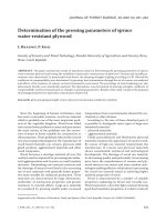
above 650 m (Fig. 1). Plots located in the third and
fourth tiers are evenly distributed along the gradi-
ent of potential global radiation, plots in the fifth
J. FOR. SCI., 56, 2010 (3): 112–120 115
tier have mainly shady aspect with lower potential
global radiation, while plots in the second tier have
mainly sunny aspect (with higher potential global
radiation) (Fig. 2).
Variability of vegetation
Phytosociological relevés were classified into
9 groups of geobiocoene types after removing
those from the nutrient-poor soils, tufa mounds
and waterlogged sites. In the 2
nd
vegetation tier
there were Fagi-querceta typica, Fagi-querceta
aceris, Fagi-querceta tiliae, in the 3
rd
vegetation
tier Querci-fageta typica, Querci-fageta aceris,
Querci-fageta tiliae, in the 4

th
ve-getation tier
Fageta typica, Fageta aceris and in the 5
th
ve-
getation tier Abieti-fageta typica and Abieti-fageta ace-
ris inferiora. Phytosociological relevés were re-
Vegetation tier
2 3 4 5
Altitude (m a.s.l.)
800
700
600
500
400
300
Vegetation tier
2 3 4 5
Potential global radiation (MWh.m
–2
per year)
2.0
1.6
1.2
Table 1. Coefficients of determination (R
2
) and significances based on permutation tests (1,000 permutations) for
variables fitted as vectors to the NMDS ordination. (e analysis was performed for 3 subsets of data: subset I included
all phytosociological relevés in which at least 2 species per plot occurred in the herb layer, subset II (at least 8 herb-layer
species per plot) and subset III (at least 14 herb-layer species per plot))

Variable
R
2
(significance)
subset I (≥ 2 species) subset II (≥ 8 species) subset III (≥ 14 species)
Cover of tree layer 0.0898 (***) 0.2210 (***) 0.3335 (***)
Elevation 0.2457 (***) 0.3247 (***) 0.4062 (***)
Slope 0.0638 (**) 0.0551 (**) 0.0391 (.)
Radiation 0.1706 (***) 0.1487 (***) 0.1486 (***)
Vegetation tiers 0.2380 (***) 0.3168 (***) 0.4670 (***)
Significance levels: ***α = 0.001. **α = 0.01. *α = 0.05. (.) α = 0.1
Fig. 2. Box-and-whisker plots showing the distribution of po-
tential global radiation in vegetation tiers determined through
field survey. Center line and outside edge (hinges) of each box
represent the median and range of inner quartile around the
median; vertical lines on the two sides of the box (whiskers)
represent values falling within 1.5 times the absolute value
of the difference between the values of the two hinges; circle
represents outside values
Fig. 1. Box-and-whisker plots showing the distribution of eleva-
tion in vegetation tiers determined through field survey. Center
line and outside edge (hinges) of each box represent the median
and range of inner quartile around the median; vertical lines on
the two sides of the box (whiskers) represent values falling within
1.5 times the absolute value of the difference between the values
of the two hinges; circle represents outside values
116 J. FOR. SCI., 56, 2010 (3): 112–120
NMDS1
–1.0 –0.5 0.0 0.5
NMDS2

0.6
0.4
0.2
0.0
–0.2
–0.4
–0.6
–0.8
2
nd
vegetation tier
3
rd
vegetation tier
4
th
vegetation tier
5
th
vegetation tier
4
3.5
3
2.5
Fig. 3. NMDS ordination plot for subset of phytosociological relevés with more than 14 species. Only species from herb layer are
used for ordination. Environmental variables (rad – potential global radiation, elev – elevation), cover of tree layer (cover_trees) and
vegetation tiers (VS) are fitted as vectors on the ordination. Vegetation tiers are fitted also as surface using GAM (grey isolines)
Fig. 4. Box-and-whisker plots showing the distribution of model
values of vegetation tiers in vegetation tiers determined through
field survey. Center line and outside edge (hinges) of each box

represent the median and range of inner quartile around the
median; vertical lines on the two sides of the box (whiskers)
represent values falling within 1.5 times the absolute value
of the difference between the values of the two hinges; circle
represents outside values
Vegetation tier
2 3 4 5
Model values
5.0
4.5
4.0
3.5
3.0
2.5
2.0
corded in forest stands with the near natural tree
species composition (mainly with Quercus petraea,
Fagus sylvatica, Carpinus betulus and Abies alba)
as well as in forest stands hardly influenced by
human activities (Picea abies and Pinus sylvestris
monocultures).
Influence of variables on vegetation
Elevation, potential global radiation, tree canopy
cover and vegetation tiers are variables which signifi-
cantly influence the herb layer species composition.
Significances and coefficients of determinations
(R
2
) for variables fitted to NMDS ordination for all
subsets of plots are shown in Table 1. Elevation and

potential global radiation fitted as vectors to NMDS
ordination are significant with P value < 0.001.
R
2

for elevation is highest in the subset of plots with at
least 14 species of herb layer (R
2

= 0.4062) and lowest
in the subset of plots with at least 2 species of herb
layer (R
2

= 0.2457). R
2

for potential global radiation is
almost the same for all 3 analyzed subsets. Another
DEM-derived variable is slope. Its influence on the
herb layer species composition is lower; it is not
statistically significant (at α = 0.05) for the subset of
records with at least 14 herb layer species per plot. e
variable ‘tree canopy cover’ is significant with P value
< 0.001 and it has the highest influence in the subset of
records with at least 14 herb layer species per plot.
J. FOR. SCI., 56, 2010 (3): 112–120 117
Fig. 5. Map of vegetation tiers derived from the model and its comparison with vegetation tiers from RPFD. Vegetation tiers from
model are based on the system of geobiocoenological typology, vegetation tiers from RPFD (Regional Plans of Forest Development)
are based on the typological system of FMI. From the map it is possible to see different concept of the 5

th
vegetation tier in the
mapping from RPFD and insufficient incorporation of vegetation inversion by the model especially in lower vegetation tiers
Part of the study area around the town Uherský Brod
Part of the study area around the towns
Valašské Klobouky and Brumov-Bylnice
Vegetation tiers (VT) from model
2 (beech-oak)
3 (oak-beech)
4 (beech)
5 (fir-beech)
area mapped as higher VT
no difference
area mapped as lower VT
Differences in VT from RPFP
km
Table 2. Error matrix for the classification of plots into vegetation tiers determined by the model and vegetation tiers
determined by a field survey. e number of plots within different categories is shown
Vegetation tiers determined by the model
Vegetation tiers determined by a field survey
2
nd
3
rd
4
th
5
th
row sum
2

nd
10 2 0 0 12
3
rd
1 46 3 0 50
4
th
0 4 55 3 62
5
th
0 0 0 14 14
Column sum 11 52 58 17 138
Vegetation tiers themselves, fitted as vectors,
have similar R
2

and similar direction as elevation
(Table 1, Fig. 3). ey represent the most significant
variable (R
2
= 0.46) in the subset of records with at
least 14 herb layer species per plot. Parameters of
the generalized additive model by which the smooth
surface of vegetation tiers is fitted are statistically
significant; the deviation explained by the model
(D
2
) is 0.49.
Model for vegetation tiers
e model for vegetation tiers in which elevation

was included as the independent variable explains
78% of variability (R
2
adj
= 0.7759, t
elev
= 21.805,
df = 136,
P
elev
< 0.001). e model with potential
global radiation explains much less variability
(R
2
adj
= 0.1416, t
rad
= –4.858, df = 136, P
rad
< 0.001).
e model in which both variables are included ex-
118 J. FOR. SCI., 56, 2010 (3): 112–120
plains 84% of variability, both variables are significant
(R
2
adj
= 0.8366, t
rad
= –7.172, df = 135, P
rad

< 0.001,
t
elev
= 24.068, df = 135, P
elev
< 0.001).
Limits between vegetation tiers were set for model
values at 2.55, 3.5 and 4.5. Model values slightly over-
lap with vegetation tiers determined by a field survey
(Fig. 4). In total 13 plots were classified differently by
the model (9% plots). In other words, 91% of plots
were classified equally (Table 2).
Comparison of model vegetation tiers
and vegetation tiers obtained from RPFD
e resulting map of model vegetation tiers cor-
responds to the map of vegetation tiers from RPFD in
64%. e lowest difference was found for the 3
rd
ve-
getation tier, the highest for the 5
th
and for the 2
nd
ve-
getation tier (Table 3, Fig. 5).
DISCUSSION
Elevation is an important variable affecting the herb
layer species composition. Its importance increases
as we select the subset of plots with a higher number
of species recorded in the plot (Table 1). is may

be explained by the higher probability of occurrence
of indicator species. However, using only the herb
layer species composition is not sufficient for accurate
determination of vegetation tiers in the study area
(Fig. 3). e herb layer species composition is affected
by a number of other variables (e.g. by canopy cover
in performed analyses). e effect of some of these
variables was excluded in this paper by excluding
phytosociological relevés from the nutrient-poor soils
(trophic range A and AB according to B, L
2007), relevés from the tufa mounds and waterlogged
sites where the determination of vegetation tier is less
obvious and the impact of vegetation tiers on vegeta-
tion composition is overlaid by the impact of these
variables (B, L 2007). Problems related to
the determination of vegetation tiers and the use of
bioindication were discussed by G and C
(2005). Vegetation tiers are often determined in forest
stands affected by forest management practices which
e.g. alter the tree species composition. ese influ-
ences can be obvious (such as spruce monocultures
at a low altitude) while others may be rather elusive
(e.g. former use of the forest as wood pasture allowing
more light to reach the forest floor).
e linear model developed for classifying vegeta-
tion tiers based on DEM-derived variables (eleva-
tion and potential global radiation) was found to be
satisfactory, explaining 84% of data variability. e
effect of both variables is linear (see Fig. 6 for eleva-
tion) in the study area. However, this could not be

necessarily valid in the whole gradient of vegetation
Fig. 6. Scatter plot of model values of vegetation tiers against
altitude. Figure shows positive linear relationship of these
variables
Table 3. Error matrix for vegetation tiers determined by the model and vegetation tiers classified by RPFD
Vegetation tiers determined by the model (area in ha)
Vegetation tiers by RPFD (area in ha)
1
st
2
nd
3
rd
4
th
5
th
row sum
1
st
0 5 4 0 0 9
2
nd
0 1,043 698 0 0 1,741
3
rd
0 292 2,110 508 4 2,914
4
th
0 0 341 1,247 204 1,792

5
th
0 0 13 507 241 761
Column sum 0 1,340 3,166 2,262 449 7,217
Elevation (m a.s.l.)
300 400 500 600 700 800
Model values of vegetation tiers
5.0
4.5
4.0
3.5
3.0
2.5
2.0
J. FOR. SCI., 56, 2010 (3): 112–120 119
tiers in the Czech Republic. Only 9% of plots (in total
13 plots) were classified differently by the model than
by the field survey, out of them 5 were close to the
border of the vegetation tier (less than 20 m), 3 were
on the bases of valleys perhaps influenced by vegeta-
tion inversion. e classification of the other 5 plots
is problematic, 2 plots are in oak stands at higher
elevation where probably more light available to the
herb layer influences the occurrence of species from
lower vegetation tiers, 2 plots are on the south facing
slopes of the 5
th
vegetation tier where only few plots
are established and 1 is close to the forest edge.
e model was used to obtain a smooth trend of

vegetation tiers, based on variables relevant to the
definition of vegetation tiers by Z (1976a).
Plots which do not fit into this trend were reclassi-
fied into another vegetation tier. Based on the com-
bination of selected variables, the model has further
extended the knowledge of vegetation tiers from
sample plots to the whole study area. It represents an
analogical approach to the site classification which is
based on similarity of the site being classified to the
analogous easily classifiable site (e.g. with the species
composition closer to that of natural conditions). is
approach is commonly known and used in mapping
not only vegetation tiers but also groups of geobio-
coene types (B, L 2007). However, the
approach presented here allowed us to obtain more
accurate and precise results more efficiently.
Elevation and global potential radiation are suf-
ficient variables for the study area. Areas with steep
valley slopes would probably require additional vari-
ables to characterize inversion areas (slightly miss-
ing also in the study area). e effect of vegetation
inversion is more important in the lower vegetation
tiers (from 1
st
to 4
th
vegetation tier) (B, L
2007). In future, the model could be improved by a
variable derived from DEM that expresses the effect
of inversion. For example A et al. (2001) used

GIS based depth in sink to estimate the distribution
of 6 dominant tree species in karst regions. Simi-
larly to model vegetation tiers in larger areas, more
variables would probably be needed (e.g. to express
varying amounts of precipitation).
Two thirds of the map of model-determined veg-
etation tiers are equivalent to the map obtained from
RPFD (Table 3, Fig. 5). is result can be considered
as satisfactory taking into account differences be-
tween vegetation tiers defined by the system of geo-
biocoenological typology and vegetation tiers defined
by the typological system of FMI. e typological
system of FMI classifies azonal forest types into lower
or higher vege-tation tiers than the surrounding
area (M 2000). M (2000) proposed
geographically zonal vegetation tiers which are more
similar to vegetation tiers in geobiocoenological ty-
pology. But these are not included in RPFD. is is
for example the cause of determination of the 1
st
ve-
getation tier in the study area by RPFD. Other dif-
ferences may be explained by a slightly different
approach to the definition of individual vegetation
tiers in both systems. e most important differ-
ences are in the 5
th
and in the 2
nd
vegetation tiers

in the study area. Differences in the mapping of the
5
th
vegetation tier can be explained by a different
concept of determination of this vegetation tier. In
the mapping for RPFD this tier is mapped from lower
altitudes in the north-eastern part of the study area
(Fig. 5). Differences in the mapping of the 2
nd
ve-
getation tier revealed insufficient incorporation of the
effect of vegetation inversion by the model.
CONCLUSION
Vegetation tiers were successfully modelled in
the study area using elevation and potential global
radiation as independent variables. Both variables
have a similar influence on the herb layer species
composition. e presented model explains 84% of
data variability. Only relatively few plots (9%) were
classified differently by the model than by the field
survey. e possibilities of using a digital elevation
model for the more accurate and efficient mapping
of vegetation tiers were explored. e findings may
be used e.g. for transferring the knowledge of veg-
etation tiers from natural forest fragments to the
whole landscape in a particular region.
R ef e re n ce s
A Z., Š J. (2001): Geobiocoenology I. Brno,
MZLU v Brně. (in Czech)
A O., H D., P R. (2001): DEM-based depth

in sink as an environmental estimator. Ecological Model-
ling, 138: 247–254.
A M.P. (1980): Searching for a model for use in vegeta-
tion analysis. Vegetatio, 42 : 11–21.
A M.P., B L., M J., D M., L M.
(2006): Evaluation of statistical models used for predicting
plant species distributions: Role of artificial data and theory.
Ecological Modelling, 199: 197–216.
B A., L J. (2007): Geobiocoenology II. Geobio-
coenological Typology of the Czech Republic Landscape.
Brno, MZLU v Brně: 251. (in Czech)
B A., L J., C M., G V. (2005): Charac-
teristics of vegetation tiers. In: C M. (ed.): Biogeographic
Division of the Czech Republic, Volume 2. Praha, Agentura
ochrany přírody a krajiny ČR: 23–60. (in Czech)
120 J. FOR. SCI., 56, 2010 (3): 112–120
C J.B. (2002): Introduction to Remote Sensing. New
York, Guilford Press: 621.
Czech Geological Survey (2003): GEOČR50, geoscience GIS
layers geodatabase of geological maps at a scale of 1:50,000)
Available at (accessed
September 10, 2007)
D B G., A B., P J., D C. (1997):
Response of high mountain landscape to topographic vari-
ables: Central Pyrenees. Landscape Ecology, 12: 95–115.
E H. (1986): Vegetation Ecology of Central Europe.
Cambridge, Cambridge University Press.
Forest Management Institute Brandýs nad Labem (2003): Re-
gional Plans of Forest Development. Available at http://www.
uhul.cz/en/oprl/index.php (wms server: l.

cz/wms_oprl?SERVICE=WMS) (accessed October 6, 2009)
G M., P H., G G. (1998): Prediction
of vegetation patterns at the limits of plant life: a new view
of the Alpine-nival ecotone. Arctic and Alpine Research,
30: 207–221.
GRASS Development Team (2009): Geographic Resources Analy-
sis Support System (GRASS GIS) Software ITC-irst, Trento,
Italy. Available at (accessed May 5, 2009)
G V., C M. (2005): Remarks to vegetation tiers.
In: C M. (ed.): Biogeographic Division of the Czech
Republic, Volume 2. Praha, Agentura ochrany přírody
a krajiny ČR: 21. (in Czech)
G A., Z N.E. (2000): Predictive habitat
distribution models in ecology. Ecological Modelling,
135: 147–186.
G A., T J.P., K F. (1998): Predicting
the potential distribution of plant species in an alpine envi-
ronment. Journal of Vegetation Science, 9: 65–74.
H A.K., E-D M.A., H H.A. (1998):
Vegetation, species diversity and floristic relations along an
altitudinal gradient in south-west Saudi Arabia. Journal of
Arid Environments, 38: 3–13.
H A. (2006): Continuum or zonation? Altitudinal gra-
dients in the forest vegetation of Mt. Kilimanjaro. Plant
Ecology, 184: 27–42.
H S.M., S J.H.J. (2001): TURBOVEG,
a comprehensive database management system for vegeta
-
tion data. Journal of Vegetation Science, 12: 589–591.
H J., Š M. (2002): e solar radiation model for Open

Source GIS: implementation and applications. In: C M.,
Z P. (eds): Proceedings of the Open Source GIS – GRASS
Users Conference 2002. Trento, Italy, 2002, 11–13 September
2002. Available at />GRASS2002/home.html (accessed March 20, 2009)
H O., H J. (2008): Characteristics of 3
rd
(Querci-
fageta s. lat.) and 4
th
(Fageta (abietis) s. lat.) vegetation tiers
of north-eastern Moravia and Silesia (Czech Republic).
Journal of Forest Science, 54: 439–451.
H R., C J. (2002): Topography and the En-
vironment. Prentice Hall, Pearson Education: 274.
C I. (2002): Geological History of the Czech Republic.
Praha, Academia. (in Czech)
K M. (2006): Optimization of digital terrain model
for its application in forestry. Journal of Forest Science,
52: 233–241.
MC B., K D. (2002): Equations for potential annual
direct incident radiation and heat load. Journal of Vegeta-
tion Science, 13: 603–606.
M M. (2000): Proposal of formation and classifica-
tion of outlines of geographically zonal vegetation tiers.
In: V J. (ed.): e Questions of Forest Typology II.
Kostelec nad Černými lesy, 11.–12. 1. 2000. Praha, ČZU,
FLE: 19–21. (in Czech)
N M., M H. (2008): Open Source GIS: A GRASS
GIS Approach. 3
rd

Ed. New York, Springer: 406.
P K.B. Jr., L T., U D. (2005): A simple
method for estimating potential relative radiation (PRR)
for landscape-scale vegetation analysis. Landscape Eco-
logy, 20: 137–147.
P K., Ž I. (1986): Natural Forest Areas in Czecho-
slovakia. Praha, Státní pedagogické nakladatelství: 313.
(in Czech)
R D., V J., P K. (1986): Phytosociology and
Forest Typology. Bratislava, Príroda: 339. (in Slovak)
Š M., H J. (2004): A new GIS-based solar radia-
tion model and its application to photovoltaic assessments.
Transactions in GIS, 8: 175–190.
T L. (2002): JUICE, software for vegetation classification.
Journal of Vegetation Science, 13: 451–453.
T R. (2007): Climate Atlas of Czechia. Praha, Olomouc,
Český hydrometeorologický ústav, Univerzita Palackého
v Olomouci: 255. (in Czech)
V J., K A., M M. (2003): Czech forest eco-
system classification. Journal of Forest Science, 49: 85–93.
Z B.P., W H.Z., X F., X J., Z Y.H. (2006):
Integration of data on Chinese Mountains into a digital
altitudinal belt system. Mountain Research and Develop-
ment, 26: 163–171.
Z A. (1963): Die Vegetationstufen und deren Indika-
tion durch Pflanzenarten am Beispiel der Wälder der ČSSR.
Preslia, 35: 31–51.
Z A. (1976a): Overview of groups of geobiocoene types
originally wooded or shrubed. Zprávy Geografického ústavu
ČSAV v Brně, 13: 55–56. (in Czech)

Z A. (1976b): Forest Phytosociology. Praha, Státní
zemědělské nakladatelství: 495. (in Czech)
Received for publication June 22, 2009
Accepted after corrections October 12, 2009
Corresponding author:
Ing. D V, Mendelova univerzita v Brně, Lesnická a dřevařská fakulta, Zemědělská 3,
613 00 Brno, Česká republika
tel.: + 420 545 134 048, fax: + 420 545 211 422, e-mail: