Báo cáo lâm nghiệp: "A linkage among whole-stand model, individual-tree model and diameter-distribution model" ppsx

600 J. FOR. SCI., 56, 2010 (12): 600–608
JOURNAL OF FOREST SCIENCE, 56, 2010 (12): 600–608
A linkage among whole-stand model, individual-tree
model and diameter-distribution model
X. Z, Y. L
Research Institute of Forest Resource Information Techniques, Chinese Academy of Forestry,
Beijing, China
ABSTRACT: Stand growth and yield models include whole-stand models, individual-tree models and diameter-distri-
bution models. In this study, the three models were linked by forecast combination and parameter recovery methods
one after another. Individual-tree models combine with whole-stand models through forecast combination. Forecast
combination method combines information from different models, disperses errors generated from different models,
and then improves forecast accuracy. And then the forecast combination model was linked to diameter-distribution
models via parameter recovery methods. During the moment estimation, two methods were used, arithmetic mean
diameter and quadratic mean diameter method (A-Q method), and arithmetic mean diameter and diameter variance
method (A-V method). Results showed that the forecast combination for predicting stand variables outperformed over
the stand-level and tree-level models respectively; A-V method was superior to A-Q method on estimating Weibull
parameters; these three different models could be linked very well via forecast combination and parameter recovery.
Keywords: forecast combination; linkage; parameter recovery; stand growth and yield model
Supported by the MOST, Projects No. 2006BAD23B02, No. 2005DIB5JI42, and No. CAFYBB2008008.
In forest management, forest growth and yield
models play a very important role in studying for-
est growth processes and predicting forest growth.
Forest growth and yield models can be classified
into three broad categories: whole-stand models,
individual-tree models, and diameter-distribu-
tion models (M 1974). Whole-stand models
are models that use the stand as a modelling unit
(C et al. 1981; L et al. 1988; T et al. 1993;
W 2006), whereas individual-tree models take
the individual tree as a studied object (Z et
al. 1997; C 2000; C et al. 2002; Z, L

2009). Diameter-distribution models, in contrast,
use statistical probability functions, such as the
Weibull function (B, D 1973; M 1988;
L et al. 2004; N et al. 2005), beta func-
tion (G-V et al. 2008) or SB function
(W, R 2005). ere are strengths and
weaknesses of each type of model. Whole-stand
models can predict stand variables directly, but
they lack detailed tree-level information. On the
other hand, individual-tree models provide more
detailed information, and diameter-distribution
models offer the stand diameter structure, but
stand-level outputs from these two types of mod-
els often suffer from an accumulation of errors and
subsequently poor accuracy and precision (M
1996; G 2001; Q, C 2006).
For further studying forest growth models, for-
esters proposed that these three types of models
should be considered to link one model to another
rather than being used completely separately. e
parameter-recovery method was used to link the
whole-stand model to the diameter-distribution
model (H, M 1983; L, M 1986)
and the individual-tree model to the diameter-
distribution model (B 1980; C 1997). A
linkage between the whole-stand model and the
J. FOR. SCI., 56, 2010 (12): 600–608 601
individual-tree model was established by the disag-
gregation method and forecast combination meth-
od to improve accuracy and compatibility (Z

et al. 1993; R, H 1997; Q, C 2006;
Y et al. 2008). However, to our knowledge, no
rigorous linkage among the three types of models
has been documented so far. e objective of this
study was to link three different models by the fore-
cast combination method and parameter-recovery
method one after another.
MATERIAL AND METHODS
e data, provided by the Inventory Institute of
Beijing Forestry, consisted of a systematic sample
of permanent plots with a 5-year re-measurement
interval. e plots, 0.067 ha each, were in Chinese
pine (Pinus tabulaeformis) plantations situated on
upland sites throughout northwestern Beijing. e
data consisted of 156 measurements, with a 5-year
re-measurement interval, obtained in the follow-
ing years: 1986, 1991, 1996 and 2001. In this study,
106 plots were used in model development, and
Table 1. Distributions of plots
Measurement time Fit data Validation data Total
1986–1991 27 12 39
1991–1996 37 17 54
1996–2001 42 21 63
Total 106 50 156
Table 2. Statistics of stand variables and tree variable
Variables
Fit data Validation data
Min Max Mean SD Min Max Mean SD
Age (years) 11 55 30 8.12 13 60 30 8.81
Dominant height (m) 0.4 17.4 6.87 2.50 2.7 17.4 7.08 3.10

No. of trees (trees·ha
–1
) 238.73 2283.58 1199.63 526.81 238.81 2089.55 1178.98 469.66
Quadratic-mean diameter (cm) 5.76 17.33 10.77 2.46 5.70 17.86 10.76 2.90
Arithmetic-mean diameter (cm) 5.73 17.01 10.33 2.30 5.66 17.43 10.40 2.79
Min-diameter (cm) 5 10.1 5.50 0.87 5 9.7 5.66 1.07
Stand basal area (m
2
·ha
–1
) 0.80 33.10 11.21 6.31 0.61 28.06 10.87 6.14
Diameter at breast (cm) 5 36.8 10.46 3.91 5 30.9 10.05 3.48
SD – standard deviation
another 50 plots for validation. Table 1 shows the
distribution of plots. Summary statistics for both
data sets are presented in Table 2.
C (2002) developed a variable rate method to
predict annual diameter growth and survival for an
individual tree. is method was based on the fact
that rates of survival and diameter growth vary from
year to year. Stand-level growth and survival were
also treated in a similar manner (O, C 2003).
Because the quadratic mean diameter (Dg) is
equal to or greater than the arithmetic mean diam-
eter (Dm) (C, M 2000), the arithme-
tic mean diameter was modelled using the equation
(D-A et al. 2006):
Dm = Dg – Exp(Xδ) (1)
where: X is the vector of stand variables (e.g. dominant
height, stand age and stand density) and δ is the vector

of parameters to be estimated.
e variable rate method was used in this study.
Annual changes in dominant height, stand sur-
vival, quadratic mean diameter, arithmetic mean
diameter, diameter standard deviation, minimum
diameter, stand basal area, diameter, and survival
probability were described in recursive manner
(O, C 2003; Q et al. 2007; C, S
2008). Table 3 lists the stand-level and tree-level
growth equations.
Estimates of individual-tree diameters at age t+q
were obtained by the tree diameter growth model
(equation 13.h) and then
T
gD
ˆ
g
T
,
T
mD
ˆ
m
T
and
T
sdD
ˆ
sd
T

were
calculated for each plot at age t+q. Stand survival
was calculated with tree survival probability.
602 J. FOR. SCI., 56, 2010 (12): 600–608
Table 3. List of the recursive stand-level and tree-level growth equations.
R
t
= (10,000 /N
t
)
0.5
/H
t
= the relative spacing at age A
t
, q = length of growth period in years (in this case, q = 5), H
t
= dominant
height in m at age A
t
, N
t
= number of trees per ha at age A
t
, D
gt
= quadratic mean diameter in cm at age A
t
, D
mt

= arithmetic
mean diameter in cm at age A
t
, B
t
= stand basal area in m
2
·ha
–1
at age A
t
, Dsd
t
= diameter standard deviation in cm at age
A
t
, Dmin
t
= minimum diameter in cm at age A
t
, D
i,t
= diameter of tree i at age A
t
, p
i,t+1
= probability that tree i is survived
the period for age A
t
to A

t+1
, α
1
, α
2
, , 
4
= parameters to be estimated
Year (t+1)
)]/)(/1()()/[(
321111 tttttttt
HAAAHLnAAExpH
α
α
α
++−+=
+++
(12.a)
)]}(/)[/1()()/{(
321111 tttttttt
NLnAAANLnAAExpN
β
β
β
+
+
−+=
+++
(12.b)
)]/)(/1()()/[(

321111 tttttttt
HAAADgLnAAExpDg
χ
χ
χ
++−+=
+++
(12.c)
])(//[
5432111 tttttt
DmHNLnAExpDgDm
δ
δ
δ
δ
δ
++++−=
++
(12.d)
)]}(/)[/1()()/{(
321111 tttttttt
NLnHAABLnAAExpB
φ
φ
φ
++−+=
+++
(12.e)
)]}()()[/1()()/{(
321111 tttttttt

NLnHLnAADsdLnAAExpDsd
γ
γ
γ
++−+=
+++
(12.f)
)]}(//)[/1()min()/{(min
321111 tttttttt
NLnAAADLnAAExpD
κ
κ
κ
++−+=
+++
(12.g)
)](///[
,543121,1, titttttiti
DLnRsBAAExpDD
λ
λ
λ
λ
λ
+++++=
++
(12.h)
1
43211,
)]}(/)(//[1{

−
+
++++=
ttttti
NLnDgLnDAExpP
μμμμ
(12.i)
Year (t + q)
)]/)(/1()()/[(
13121111 −+−++−+−++−++
++−+=
qtqtqtqtqtqtqtqt
HAAAHLnAAExpH
α
α
α
(13.a)
)]}(/)[/1()()/{(
13121111 −+−++−+−++−++
++−+=
qtqtqtqtqtqtqtqt
NLnAAANLnAAExpN
β
β
β
(13.b)
)]/)(/1()()/[(
13121111 −+−++−+−++−++
++−+=
qtqtqtqtqtqtqtqt

HAAADgLnAAExpDg
χ
χ
χ
(13.c)
)])(//[
151413121 −+−+−+−+++
++++−=
qtqtqtqtqtqt
DmHNLnAExpDgDm
δ
δ
δ
δ
δ
(13.d)
)]}(/)[/1()()/{(
13121111 −+−++−+−++−++
++−+=
qtqtqtqtqtqtqtqt
NLnHAABLnAAExpB
φ
φ
φ
(13.e)
)]}()()[/1()()/{(
13121111 −+−++−+−++−++
++−+=
qtqtqtqtqtqtqtqt
NLnHLnAADsdLnAAExpDsd

γγγ
(13.f )
)]}(//)[/1()min()/{(min
13121111 −+−++−+−++−++
++−+=
qtqtqtqtqtqtqtqt
NLnAAADLnAAExpD
κ
κ
κ
(13.g)
)](///[
1,514131211,, −+−+−++−+−++
+++++=
qtiqtqtqtqtqtiqti
DLnRsBAAExpDD
λ
λ
λ
λ
λ
(13.h)
1
14113121,
)]}(/)(//[1{
−
−+−+−+−++
++++=
qtqtqtqtqti
NLnDgLnDAExpP

μμμμ
(13.i)
J. FOR. SCI., 56, 2010 (12): 600–608 603
1–
Since cross-equation correlations existed among er-
ror components of the above models, to eliminate the
bias and inconsistency of the regression system (equa-
tion a–h), the method of seemingly unrelated regres-
sion (SUR) was used to simultaneously estimate the
regression system (equation a–h). is method was
widely used in econometrics (J 1991) and
in forest biometrics (B, B 1986; B-
 1989; O, C 2003). e fitting procedure
involved the use of option SUR of the SAS procedure
model. Parameters of the tree survival equation were
separately estimated by use of NLIN procedure.
Forecast combination
Forecast combination, introduced by B and
G (1969), is a good method for improv-
ing forecast accuracy (N et al. 1987). e
method combines information generated from dif-
ferent models and disperses errors from these mod-
els, thus improves consistency for outputs from
different models. Y et al. (2008) and Z et
al. (2009) applied forecast combination to combine
models from stand-level and tree-level. e fore-
cast combination model is expressed as follows:
Y
C
= ωY

T
+ (1–ω)Y
S
(2)
us, the variance of the forecast combination is
as follows:
σ
C
2
= ω
2
σ
T
2
+ (1–ω)
2
σ
S
2
+ 2ω(1–ω)σ
TS
(3)
According to the method of calculating weights,
a variance and covariance method was used broad-
ly (Z et al. 2006; Y et al. 2008):
2
22
2
S TS
T S TS

ss
w
ss s
-
=
+-
(4)
2
22
1
2
T TS
T S TS
ss
w
ss s
-
-=
+-
(5)
where:
C
Y

– combined estimates of stand variables,
T
Y
–
estimates of stand variables at tree-level,
S

Y
– estimates of stand variables at stand-level,
w
– weight factor,
2
T
σ
– variance of stand variables at tree-level,
2
S
σ
– variance of stand variables at stand-level,
σTS – covariance of stand variables between the tree-
level and stand-level.
Parameter-recovery method
e Weibull function has been extensively ap-
plied in forestry because of its flexibility in describ-
ing a wide range of unimodal distributions and the
relative simplicity of parameter estimation (B,
σ σ
σ σ σ
σ σ
σ σ
σ
–
–
–
1–ω
–
ω

ω
1
( ; , , ) ( ) exp[ ( ) ]
cc
cxa xa
f xabc
bb b
-

=-





=Γ−−+
Γ−=
0
ˆ
2
ˆ
/)
ˆ
(
2
222
1
bmDaagD
amDb
⎪

⎩
⎪
⎨
⎧
=Γ−−+
Γ−=
0
ˆ
2
ˆ
/)
ˆ
(
2
222
1
bmDaagD
amDb
1
D 1973; K, M 2000; M-
 et al. 2002; L 2008). e Weibull probability
density function is expressed as follows:
(a ≤ x ≤ ∞) (6)
where:
x – diameter at breast height,
a – the location parameter,
b – the scale parameter,
c – the shape parameter.
Moment estimation is one of the methods about
parameter recovery for estimating Weibull param-

eters and has been used broadly (L et al. 2004;
L 2008). Considering that the location parameter
(a) must be smaller than the predicted minimum
diameter (
min
ˆ
D
) in the stand, we set
min
ˆ
5.0 Da =

since F (1981) found that this resulted in
minimum errors in terms of goodness of fit.
Two methods were used to recover b and c in the
moment estimation. Method 1 is arithmetic mean
diameter (
ˆ
Dm
) and quadratic mean diameter (
ˆ
Dg
)
method (A-Q method) as follows (L et al. 2004):
(7)
where: Г
1
= Г(1 + 1/c), Г
2
= Г(1 + 2/c).

Method 2 is arithmetic mean diameter and di-
ameter variance (
ˆ
varD
) method (A-V method)
(D-A et al. 2006; Q et al. 2007). A
possible problem of method 1 is that
ˆ
Dg
might be
too close to or too far from
ˆ
Dm
, and can even be
smaller than
ˆ
Dm
if not properly constrained. e
resulting Weibull parameters are sensitive to the
difference between
ˆ
Dm
and
ˆ
Dg
, resulting in un-
stable estimators of b and c. e A-V method is ex-
pressed as follows:

(8)

Finally, the forecast combination combines stand
variables from tree-level and stand-level models to
predict
ˆ
C
Dg
,
ˆ
C
Dm
,
ˆ
C
Dsd
,
ˆ
min
C
D
and
ˆ
C
N
; and then Weibull
parameters b and c were estimated using the stand
variables of the forecast combination models based on
the two moment methods (equations 7 and 8). More
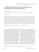
detailed procedures of this study are shown in Fig. 1.
Model evaluation
Model evaluation was performed for both growth

models and goodness of fit for the diameter distri-
bution model. For growth models, the following
evaluation statistics were calculated:





=Γ−Γ−
Γ−=
0)(var
ˆ
/)
ˆ
(
2
12
2
1
bD
amDb
⎪
⎩
⎪
⎨
⎧
=Γ−−+
Γ−=
0
ˆ

2
ˆ
/)
ˆ
(
2
222
1
bmDaagD
amDb
1
604 J. FOR. SCI., 56, 2010 (12): 600–608

Forecast
combination
A-Q
method
A-V
method
Moment
estimation
Figure 1. Flow chart
Weibull function
at age
qt
A
+
Weibull function
at age
qt
A
+
C
gD
ˆ
C
mD
ˆ
C
sdD
ˆ
C

N
ˆ
C
D min
ˆ
Tree list at age
t
A and
qt
A
+
Models at tree-level
(diameter, survival)
Models
at stand-level
T
gD
ˆ
T
mD
ˆ
T
sdD
ˆ

T
N
ˆ

T

D mi
n
ˆ
at age
qt
A
+
S
gD
ˆ
S
mD
ˆ
S
sdD
ˆ
S
N
ˆ
S
D min
ˆ
at age
qt
A
+
Fig. 1. Flow chart
R-square
R
2

= 1–∑(y
i
–ŷ
i
)
2
/ ∑ (y
i
–ŷ
i
)
2
(9)
Log Likelihood
–2ln(L) = –2{∑p
i
ln(p
i
) + ∑(1–p
i
)ln(1–p
i
)} (10)
and the evaluation of goodness of fit is error index
(e), expressed as follows (R et al. 1988; L
et al. 2004):
∑
−=
m
j

jj
OPe
(11)
where:
y
i
– observed value at age
qt
A
+
of stand variables
(arithmetic mean diameter, quadratic mean
diameter, diameter standard deviation, mini-
mum diameter or number of trees) or diameter
of tree i,
ˆ
i
y
,
i
y

– predicted value and average of y
i
, respectively,
p
i
– probability of tree i survival,
m – number of classes for each plot,
P

j

, O
j
– the predicted and observed number of trees per
plot within each diameter class j, respectively.
RESULTS AND DISCUSSION
e estimates and standard deviation errors of
parameters of the different growth models are pre-
sented in Table 4. e estimates and standard de-
viation errors showed that all the parameters were
significant (P-value < 0.0001), and R
2
values were
0.9266, 0.8983, 0.8787, 0.5392, 0.8802 and 0.9148
for the quadratic mean diameter model, arithmetic
mean diameter model, diameter standard deviation
model, minimum diameter model, stand survival
model and diameter growth model at the stand lev-
el, respectively. Log-likelihood of the tree survival
model was –782.104.
Table 5 summarizes the gains in efficiency of stand
variable models from tree-level, stand-level and
forecast combination (e.g. Y et al. 2008). For the
data subset used for fitting the models, the efficiency
for the combined quadratic mean diameter estima-
tor was 100, as compared to 100.83, 104.38 for the
tree-level and stand-level, and
2
C

σ
for the combined
estimator was 0.3977 versus 0.4010, 0.4151; the ef-
ficiency for the arithmetic mean diameter was 100,
as compared to 97.99, 119.03, and
2
C
σ
was 0.4219
vs. 0.4134, 0.5022; the efficiency for the diameter
standard deviation was 100, as compared to 105.11,
103.03, and
2
C
σ
was 0.0958 versus 0.1007, 0.0987;
the efficiency for the minimum diameter was 100,
–
J. FOR. SCI., 56, 2010 (12): 600–608 605
as compared to 121.77, 101.57, and
2
C
σ
was 0.3749
versus 0.4565, 0.3808; the efficiency for the stand
survival was 100, as compared to 111.91, 100.015,
and
2
C
σ

was 26,494.03, versus 29,648.46, 26,535.09.
Overall, except one, the combined estimators were
better than those from tree-level and stand-level
models for both fit and validation data. e only
exception was the arithmetic mean diameter model
for the fit data. Fig. 2 illustrates the relationships be-
tween the observed quadratic mean diameter and
predicted value by the three models for the valida-
tion data. It is obvious that the forecast combination
achieved the beneficial effect of the highest value R
2

(taking quadratic mean diameter as an example).
e combined predictions were based on the opti-
mal weights which are derived by the variance-co-
variance method (N, G1974) of the
two respective level models. erefore, these esti-
mators performed minimum variance and high pre-
cision (B, G 1969; J, K 2009) in
comparison with the single levels.
Table 6 shows the average values and standard de-
viations of error index (e) calculated by two different
moment estimation methods. For the data subset
used for fitting the models, the average error index
value for A-Q method was 509.7407, as compared to
442.1898 for A-V method. SD was 285.1731 versus
254.4337. Obviously, the average error index value
and SD of A-V method are much smaller than those
of A-Q method for both fit and validation data, re-
spectively. And in the fit data, Weibull parameters

of all plots (106 plots) were estimated based on A-V
method. But parameters of only 96 plots were esti-
mated by A-Q method. It means that parameters of
Table 4. Parameter estimates and model evaluation
Attribute Parameter Estimate SE R
2
Quadratic – mean diameter (cm)
(equation13.c)
χ
1
3.3940 0.0191
0.9266
χ
2
–10.5788 0.3026
χ
3
0.0094 0.0015
Arithmetic – mean diameter (cm)
(equation 13.d)
δ
1
–3.9549 0.1169
0.8983
δ
2
–27.5352 1.1346
δ
3
21.2138 0.6141

δ
4
0.0258 0.0024
δ
5
0.0733 0.0038
Diameter std. (cm)
(equation 13.f)
γ
1
1.4519 0.0952
0.8787
γ
2
0.5065 0.0187
γ
3
–0.0840 0.0135
Minimum diameter (cm)
(equation 13.g)
κ
1
1.9212 0.0975
0.5392
κ
2
–8.6532 0.6425
κ
3
3.1075 0.6983

Stand survival (trees·ha
–1
)
(equation 13.b)
β
1
2.7193 0.1625
0.8802
β
2
17.8950 0.6520
β
3
0.5664 0.0215
Diameter at breast (cm)
(equation 13.h)
λ
1
16.0367 0.8744
0.9148
λ
2
–17.2105 0.9013
λ
3
–0.0317 0.0029
λ
4
0.1382 0.0166
λ

5
–1.4525 0.1415
Tree survival
(equation 13.i)

1
7.6063 1.3892
–782.104
(–2lnL)

2
–102.9 12.7234

3
–0.3895 0.0607

4
–45.0114 8.9032
SE – standard error, R
2
– multiple coefficient of determination
606 J. FOR. SCI., 56, 2010 (12): 600–608
Table 5. Evaluation statistics from different models for fit data and validation data
Attributes
σ
2
Efficiency (%)
fit validation fit validation
Tree-level model
Quadratic mean diameter (cm) 0.4010 0.3340 100.83 103.50

Arithmetic mean diameter (cm) 0.4134 0.3407 97.99 101.73
Diameter standard deviation (cm) 0.1007 0.1252 105.11 101.95
Minimum diameter (cm) 0.4565 0.5454 121.77 100.31
Stand survival (trees·ha
–1
) 29,648.46 39,805.53 111.91 102.72
Stand-level model
Quadratic mean diameter (cm) 0.4151 0.4789 104.38 148.40
Arithmetic mean diameter (cm) 0.5022 0.6070 119.03 181.25
Diameter standard deviation (cm) 0.0987 0.1305 103.03 106.27
Minimum diameter (cm) 0.3808 0.6929 101.57 127.44
Stand survival (trees·ha
–1
) 26,535.09 41,340.33 100.15 106.68
Forecast
combination
model
Quadratic mean diameter (cm) 0.3977 0.3227 100 100
Arithmetic mean diameter (cm) 0.4219 0.3349 100 100
Diameter standard deviation (cm) 0.0958 0.1228 100 100
Minimum diameter (cm) 0.3749 0.5437 100 100
Stand survival (trees·ha
–1
) 26,494.03 38,751.85 100 100
Efficiency at tree-level = 100σ
2
T
, /σ
2
C

efficiency at stand-level = 100σ
2
S
/σ
2
C
, efficiency from forecast combination
=100σ
2
C
/σ
2
C
, and Value in bold denotes the best statistic among models for each of the fit and validation data sets
the other 10 plots could not be estimated. It was be-
cause
ˆ
C
Dg
was smaller than
ˆ
C
Dm
of those 10 plots.
e formula for diameter variance is,
D
var

=E(D
2

)–E(D)
2
and
()E D Dm=
,
22
)( DgDE =

Dg
2

E(x) is the expected value. And D
var
> 0, then
Dg Dm>
. When
Dg
is closer to
Dm
, D
var
ap-
proaches 0, and distribution shrinks to a point at
Dg
. is kind of Weibull distribution does not ex-
ist. So when
Dg
is closer to
Dm
or

Dg
is smaller
than
Dm
, Weibull parameters could not be estimat-
ed by A-Q method. It also verified the fact that it
was not suitable to use A-Q method for estimating
Weibull parameters. So A-V method outperforms
A-Q method in estimating Weibull parameters.
Fig. 2. Relationships between the observed quadratic mean
diameter and the predicted value with three models for the
validation data

y = 0.9557x - 0.5756
R
2
= 0.9611
0
5
10
15
20
0 5 10 15 20
Dg
2
-observed
Dg
2
-predicted
y = 0.916x - 0.289
R
2
= 0.9451
0
5
10
15

20
0 5 10 15 20
Dg
2
-observed
Dg
2
-predicted
y = 0.9702x - 0.6803
R
2
= 0.9624
0
5
10
15
20
0 5 10 15 20
Dg
2
-observed
Dg
2
-predicted
a: Tree level model b: Stand-level model
c: Forecast combination model
Figure 2. Relationships between the observed quadratic mean diameter and
the predicted value with three models for the validation data
y = 0.9557x–0.5756
R

2
= 0.9611
Table 6. Error index based on A-Q method and A-V method
Attribute A-Q A-V
Fit data
Mean 509.7407 442.1898
SD 285.1731 254.4337
Validation data
Mean 533.5493 479.4961
SD 286.4376 240.311
SD – standard deviation
Dg
2
observed

y = 0.9557x - 0.5756
R
2
= 0.9611
0
5
10
15
20
0 5 10 15 20
Dg
2
-observed
Dg
2
-predicted
y = 0.916x - 0.289
R
2
= 0.9451
0
5

10
15
20
0 5 10 15 20
Dg
2
-observed
Dg
2
-predicted
y = 0.9702x - 0.6803
R
2
= 0.9624
0
5
10
15
20
0 5 10 15 20
Dg
2
-observed
Dg
2
-predicted
a: Tree level model b: Stand-level model
c: Forecast combination model
Figure 2. Relationships between the observed quadratic mean diameter and
the predicted value with three models for the validation data

y = 0.9702x–0.6803
R
2
= 0.9624
Dg
2
observed
Dg
2
– predicated
Dg
2
– predicated

y = 0.9557x - 0.5756
R
2
= 0.9611
0
5
10
15
20
0 5 10 15 20
Dg
2
-observed
Dg
2
-predicted
y = 0.916x - 0.289
R
2
= 0.9451
0
5
10

15
20
0 5 10 15 20
Dg
2
-observed
Dg
2
-predicted
y = 0.9702x - 0.6803
R
2
= 0.9624
0
5
10
15
20
0 5 10 15 20
Dg
2
-observed
Dg
2
-predicted
a: Tree level model b: Stand-level model
c: Forecast combination model
Figure 2. Relationships between the observed quadratic mean diameter and
the predicted value with three models for the validation data
y = 0.916x–0.289

R
2
= 0.9451
Dg
2
observed
Dg
2
– predicated
J. FOR. SCI., 56, 2010 (12): 600–608 607
CONCLUSIONS
In this study, the forecast combination was used
to link tree-level models and stand-level models. It
efficiently utilizes information generated from dif-
ferent models, reduces errors from a single mod-
el, and improves accuracy and precision. It also
ensures that stand variables from tree-level and
stand-level models are consistent.
Forecast combination models and diameter dis-
tribution models were linked through the parame-
ter recovery method (moment estimation), and the
two moment estimation methods were used in this
study. It is much more suitable to estimate Weibull
parameters on the basis of A-V method than A-Q
method. And if
ˆ
Dm
is larger than
ˆ
Dg

or too close to
ˆ
Dg
, Weibull parameters will not be estimated by
A-Q method, but they will be estimated by A-V
method. So A-V method is superior to A-Q meth-
od for estimating Weibull parameters.
Whole-stand models, individual-tree models and
diameter models can be linked together through
the forecast combination method and the param-
eter-recovery method one after another. erefore,
this study provided a framework for studying the
integrated system of forest models.
Acknowledgements
e authors would like to thank the Inventory In-
stitute of Beijing Forestry for its data and Dr. Q
V. C for providing his information and SAS code.
References
B J.M., G C.W.J. (1969): e combination of
forecasts. Operation Research Quarterly, 20: 451–468.
B R.L., D T.R. (1973): Quantifying diameter dis-
tributions with the Weibull distribution. Forest Science,
19: 97–104.
B R.L. (1980): Individual tree growth derived from
diameter distribution models. Forest Science, 26: 626–632.
B B.E., B R.L. (1986): A compatible system of
growth and yield equations for Slash Pine fitted with restrict-
ed three-stage least squares. Forest Science, 32: 185–201.
B B.E. (1989): Systems of equations in forest stand
modeling. Forest Science, 35: 548–556.

C Q.V. (1997): A method to distribute mortality in di-
ameter distribution models. Forest Science, 43: 435–442.
C Q.V. (2000): Prediction of annual diameter growth and
survival for individual trees from periodic measurements.
Forest Science, 46: 127–131.
C Q.V., L.S.S., MD M.E. (2002): Developing a system
of annual tree growth equations for the loblolly pine–
shortleaf pine type in Louisiana. Canadian Journal Forest
Research, 32: 2051–2059.
C Q.V., S M. (2008): Evaluation of four methods to
estimate parameters of an annual tree survival and diam-
eter growth model. Forest Science, 6: 617–624.
C R.O., C G.W, R D.L. (1981): A
New Stand Simulator for Coast Douglas-Fir: DFSIM User’
Guide. General Technical Report PNW–128. Portland,
USDA Forest Service, Pacific Northwest Forest and Range
Experiment Station.
C R.O., M D.D. (2000): Why quadratic mean
diameter? West Journal of Applied Forest, 15: 137–139.
D–A U., D F.C., Á-G
J.G., A A.R. (2006): Dynamic growth model for
Scots pine (Pinus sylvestris L.) plantations in Galicia (north-
western Spain). Ecological Modelling, 191: 225–242.
F J.R. (1981): Compatible Whole-Stand and Diameter
Distribution Models for Loblolly Pine Plantations. [Ph.D.
esis.] Blackburg, Virginia Polytechnic Institute and State
University, School of Forestry and Wildlife: 125.
G O. (2001): On bridging the gap between tree–level
and stand-level models. Available at c.
ca/~garcia/publ/greenw.pdf (accessed on June 13, 2009)

G-V J.J., R-A A., A-K E.,
B-A (2008): Modelling diameter distributions of
birch (Betula alba L.) and pedunculate oak (Quercus robur
L.) stands in northwest Spain with the Beta distribution.
Investigation Agraria: Sistemas y recursos Forestales, 17:
271–281.
H D.M., M J.W. (1983): A generalized framework
for projecting forest yield and stand structure using diam-
eter distribution. Forest Science, 29: 85–95.
J D.I., K Y.O. (2009): Combining single–value stream-
flow forecasts – A review and guidelines for selecting
techniques. Journal of Hydrology, 377: 284–299.
J J. (1991): Econometric Methods. McGraw-Hill,
Singapore: 568.
K, A., M M. (2000): Calibrating predicted
diameter distribution with additional information. Forest
Science. 46: 390–396.
L Y. (2008): Evaluation of three methods for estimating the
Weibull distribution parameters of Chinese Pine (Pinus
tabulaeformis). Journal of Forest Science, 54: 549–554.
L X.F., T S.Z., W S.L. (1998): e Establishment of
variable density yield table for Chinese plantation in Da-
gangshan Experiment Bureau. Forest research, 4: 382–389.
(in Chinese)
L C.M., Z S.Y., L Y., N P.F., Z L.J.
(2004). Evaluation of three methods for predicting diameter
distributions of black spruce (Picea mariana) plantations
in central Canada. Canadian Journal Forest Research, 34:
2424–2432.
608 J. FOR. SCI., 56, 2010 (12): 600–608

L T.B., M J.W. (1986): A growth model for mixed
species stands. Forest Science, 32: 697–706.
M D., M M., K A. (2002): Predict-
ing and calibrating diameter distributions of Eucalyptus
grandis (Hill) Maiden plantations in Zimbabwe. New
Forests, 23: 207–223.
M X.Y. (1988): A study of the relation between D and
H- distributions by using the Weibull function. Journal of
Beijing Forestry University, 10: 40–47. (in Chinese)
M X.Y. (1996): Natural Resources Measurement. 2
nd
Ed.
Beijing: China Forestry Publishing House: 296. (in Chinese)
M D.D. (1974): Forest growth models – a prognosis.
In: F J. (ed.): Growth Models of Tree and Stand Simu-
lation. Royal College of Forestry, Research Note No. 30,
Stockholm.
N P., G C.W.J. (1974): Experience with forecast-
ing univariate time series and the combination of forecasts.
Journal of the Royal Statistical Society Series A, 137: 131–165.
N P., Z J.K., K S. (1987): Combining
forecasts to improve earnings per share prediction: and
examination of electric utilities. International Journal of
Forecasting, 3: 229–238.
N P.F., L Y., Z S.Y. (2005): Stand–level diam-
eter distribution yield model for black spruce plantations.
Forest Ecology and Management, 209: 181–192.
O C Q.V. (2003): A comparison of compatible and an-
nual growth models. Forest Science, 49: 285–290.
Q J.H., C Q.V. (2006): Using disaggregation to link

individual-tree and whole-stand growth models. Canadian
Journal of Forest Research, 36: 953–960.
Q J.H., C Q.V., B D.C. (2007): Projection of a
diameter distribution through time. Canadian Journal of
Forest Research, 37: 188–194.
R M.R., B T.E., H W.C. (1988): Goodness-
of-fit tests and model selection procedures for diameter
distribution models. Forest Science, 34: 373–399.
R M.W., H D.W. (1997): Implications of disag-
gregation in forest growth and yield modeling. Forest
Science, 43: 223–233.
T S.Z., L X.F., M Z.H. (1993): e development
of studies on stand growth models. Forest Research, 8:
672–679. (in Chinese)
W M.L., R K. (2005): Tree diameter distribu-
tion modeling: introducing the logit-logistic distribution.
Canadian Journal Forest Research, 35: 1305–1313.
W Z.C. (2006): Application of stand models Larix olgensis
plantations. Journal of Northeast Forestry University, 34:
31–33. (in Chinese)
Y C.F., K U., H S. (2008): Combining tree–and
stand–level models: a new approach to growth prediction.
Forest Science, 54: 553–566.
Z L., M J.A., N J.D. (1993): Disaggre-
gating stand volume growth to individual trees. Forest
Science, 39: 295–308.
Z L., P K.C., L C. (2003): A comparison of
estimation methods for fitting Weibull and Johnson’s SB
distributions to mixed spruce–fir stands in northeastern
North America. Canadian January Forest Research, 33:

1340–1347.
Z S., A R.L., B H.E. (1997): Constrain-
ing individual tree diameter increment and survival models
for loblolly pine plantations. Forest Science, 43: 414–423.
Z X.Q., LY.C. (2009): Comparison of annual individu-
al–tree growth models based on variable rate and constant
rate methods. Forest Research, 22: 824–828. (in Chinese)
Z X.Q., LY.C., C X.M, W J Z. (2010): Predic-
tion of stand basal area with forecast combination. Journal
of Beijing Forestry University. (in press)
Z Y., M C.S., W K. (2006): e study of estimation
of weight coefficient in combination forecast models – the
application of the least absolute Value model. Journal of
Transportation Systems Engineering and Information
Technology, 6: 125–129. (in Chinese)
Received for publication October 13, 2010
Accepted after corrections April 12, 2010
Corresponding author:
Prof. Doctor Y L, Chinese Academy of Forestry, Research Institute Resource Information and Techniques,
Beijing 100091, P. R. China
tel: + 86 106288 9199, fax: + 86 106288 8315, e-mail: ,