Communication Systems Engineering Episode 1 Part 3 docx
Bạn đang xem bản rút gọn của tài liệu. Xem và tải ngay bản đầy đủ của tài liệu tại đây (117.88 KB, 12 trang )
Lecture 3: The Sampling Theorem
Eytan Modiano
AA Dept.
Eytan Modiano
Slide 1
Sampling
• Given a continuous time waveform, can we represent it using
discrete samples?
– How often should we sample?
– Can we reproduce the original waveform?
�
�
�
�
�
�
�
�
�
�
Eytan Modiano
Slide 2
The Fourier Transform
• Frequency representation of signals
∞
() =
∫
−∞
x(t)e
− jft
dt
• Definition:
Xf
2
π
∞
2
π
xt() =
∫
−∞
X( f )e
jft
df
• Notation:
X(f) = F[x(t)]
X(t) = F-1 [X(f)]
x(t) � X(f)
Eytan Modiano
Slide 3
δδ
δ
Unit impulse
δ
(t)
t 0,
δ
() =∀t ≠ 0
∞
δ
() =1
∫
−∞
t
∞
δ
() () = x(0)
∫
−∞
txt
∫
∞
δ
(t −
τ
)x(
τ
) = x(t)
−∞
δ
∞
2
π
t
F[(t)]
δ
F[(t)] =
∫
−∞
δ
(t)e
− jft
dt = e
0
= 1
δ
()
t
δ
() ⇔ 1
0
Eytan Modiano
Slide 4
1
jt jf
Rectangle pulse
t
1 ||< 1/ 2
t / /
Π() =
12 | t |= 12
0 otherwise
12
Π
∞
2
π
/
F[(t)]
=
∫
−∞
Π(t)e
− jft
dt
=
∫
−12
e
− j 2
π
ft
dt
/
e
−
π
−
e
π
π
f
= =
Sin()
=
Sinc f
−
jf
π
f
2
π
()
Π()t
1
1/2 1/2
Eytan Modiano
Slide 5
αα
α
ββ
β
αα
α
ββ
β
ττ
τ
ππ
π
ττ
τ
Properties of the Fourier transform
• Linearity
– x1(t) <=> X1(f), x2(t) <=>X2(f) =>
α
x1(t) +
β
x2(t) <=>
α
X1(f) +
β
X2(f)
• Duality
– X(f) <=> x(t) => x(f) <=> X(-t) and x(-f)<=> X(t)
• Time-shifting: x(t-
τ
) <=> X(f)e
-j2
π
f
τ
• Scaling: F[(x(at)] = 1/|a| X(f/a)
• Convolution: x(t) <=> X(f), y(t) <=> Y(f) then,
– F[x(t)*y(t)] = X(f)Y(f)
– Convolution in time corresponds to multiplication in frequency and
visa versa
∞
xt xt −
τ
)y(
τ
)d
τ
()* y(t) =
∫
−∞
(
Eytan Modiano
Slide 6
ΠΠ
Π
ππ
π
ΠΠ
Π
ΠΠ
Π
Fourier transform properties (Modulation)
2
π
xt e
jf
o
t
⇔ X( f − f
o
)()
e
jx
+ e
− jx
Now, cos(x) =
2
xt e
jf
o
t
+ x t e
− j 2
π
f
o
t
xt() cos(
2
π
f
o
t) =
()
2
π
()
2
(
x tHence,( ) cos(
2
π
f
o
t) ⇔
Xf − f
o
) + X( f + f
o
)
2
• Example: x(t)= sinc(t), F[sinc(t)] =
Π
(f)
• Y(t) = sinc(t)cos(2
π
f
o
t) <=> (
Π
(f-f
o
)+
Π
(f+f
o
))/2
1/2
Eytan Modiano
-f
o
+f
o
Slide 7
|(
More properties
• Power content of signal
• Autocorrelation
• Sampling
Eytan Modiano
Slide 8
∫
∞ ∞
xt
−∞
|( ) |
2
dt =
∫
−∞
Xf ) |
2
df
∞
*
R
x
() =
∫
−∞
x(t)x (t −
τ
)dt
τ
R
x
() ⇔ | X( f ) |
2
τ
xt
o
( )
δ
(t − t
o
)() = xt
∞
xt()
∑
δ
(t − nt
o
) = sampled version of x(t)
n =−∞
∞ ∞
F[
∑
δ
(t − nt
o
)] =
1
∑
δ
( f −
n
)]
t t
n
=−∞
o
n
=−∞
o
The Sampling Theorem
Xf()
() = 0, for all f ,| f | ≥ W
• Band-limited signal
Xf
– Bandwidth < W
-w
w
Sampling Theorem: If we sample the signal at intervals Ts where
Ts <= 1/ 2W then signal can be completely reconstructed from its
samples using the formula
∞
xt() =
∑
2W
©
T
s
x(nT
s
)sin c[2W
©
(t − nT
s
)]
n =−∞
Where, W ≤ W
©
≤
1
− W
T
s
∞
1
t
WithT = => xt
s
() =
∑
x(nT
s
)sin c[( − n)]
2
W T
n =−∞
s
∞
n n
() =
∑
x( )sin [
2
xt cW(t − )]
2
W
2
W
n =−∞
Eytan Modiano
Slide 9
Proof
∞
xt ()
∑
δ
(t
−
nT
s
)
δ
()
=
x t
n =−∞
∞
Xf ()* F[
∑
δ
(t
−
nT
s
)]
δ
()
=
X f
n
=−∞
∞ ∞
F[
∑
δ
(t
−
nT
s
)]
=
1
∑
δ
( f
−
n
)
n
=−∞
T
s
n
=−∞
T
s
1
∞
n
δ
()
=
∑
Xf
−
)Xf (
Ts
n
=−∞
T
s
• The Fourier transform of the sampled signal is a replication of the
Fourier transform of the original separated by 1/Ts intervals
-1/Ts
-w
w
1/Ts
2/Ts
Eytan Modiano
Slide 10
Proof, continued
• If 1/Ts > 2W then the replicas of X(f) will not overlap and can be
recovered
• How can we reconstruct the original signal?
– Low pass filter the sampled signal
f
• Ideal low pass filter is a rectangular pulse
Hf T() =Π( )
s
2W
• Now the recovered signal after low pass filtering
f
Xf f T
() = X
δ
()
s
Π( )
2W
f
xt
() = F
−1
[ X
δ
( f )T
s
Π( )]
2W
∞
t
() =
∑
xnT
s
)Sinc( − n)xt (
n
=−∞
T
s
Eytan Modiano
Slide 11
Notes about Sampling Theorem
• When sampling at rate 2W the reconstruction filter must be a
rectangular pulse
– Such a filter is not realizable
– For perfect reconstruction must look at samples in the infinite future
and past
• In practice we can sample at a rate somewhat greater than 2W
which makes reconstruction filters that are easier to realize
• Given any set of arbitrary sample points that are 1/2W apart, can
construct a continuous time signal band-limited to W
Eytan Modiano
Slide 12