Compressor Instability with Integral Methods Episode 1 Part 5 doc

Chapter 3
Air and Abrasive Acceleration
3.1 Properties of Compressed Air
Air is a colourless, odourless and tasteless gas mixture. It consists of many gases, but
primarily of oxygen (21%) and nitrogen (78%). Air is always more or less contam-
inated with solid particles, for example, dust, sand, soot and salt crystals. Typical
properties of air are listed in Table 3.1. If air is considered to be an ideal gas, its
behaviour can be described based on the general law of state:
p · υ
S
= R
i
· T (3.1)
where p is the static air pressure, υ
S
is the specific volume of the gas, R
i
is the
individual gas constant and T is the absolute temperature. It can be distinguished
between three pressure levels, which are illustrated in Fig. 3.1. The relationships
between these pressure levels are as follows:
p = p
0
+ p
G
(3.2)
The parameter p is the absolute pressure, the parameter p
G
is the gauge pressure
usually read by the pressure gages in the blast cleaning pressure systems, and the
parameter p

0
is the atmospheric pressure. The atmospheric pressure is a function of
altitude. It is important not to confuse the absolute pressure and the gauge pressure.
For theoretical calculations, the absolute pressure must be used.
The parameter R
i
in (3.1) is the individual gas constant, which is the energy de-
livered by a mass of 1 kg of air if its temperature is increased by +1
◦
C (K) at constant
pressure. Its value for air is provided in Table 3.1. The individual gas constant is the
difference between isobaric heat capacity and isochoric heat capacity of the gas:
R
i
= c
P
− c
V
(3.3)
The ratio between isobaric heat capacity and isochoric heat capacity is the isen-
tropic exponent of the gas:
κ =
c
P
c
V
(3.4)
A. Momber, Blast Cleaning Technology 55
C


Springer 2008
56 3 Air and Abrasive Acceleration
Table 3.1 Properties of air
Parameter Symbol Unit Value
Density
a
ρ
A
kg/m
3
1.225
Dynamic viscosity
a
η
0
Ns/m
2
1.72 × 10
−5
Isobaric specific heat capacity
b
c
P
Nm/(kg K) 1,004
Isochoric specific heat capacity
b
c
V
Nm/(kg K) 717
Gas constant R

i
Nm/(kg K) 287
Adiabatic exponent κ –1.4
Critical pressure ratio β – 0.528
Kinematic viscosity ν
A
m
2
/s 1.82 × 10
−5
Specific evaporation heat q
V
Nm/kg 1.97 × 10
−5
Speed of sound
a
c m/s 331
Sutherland parameter C
S
K 113
a
Thermodynamic standard (Table 3.2: ϑ = 0
◦
C, p = 0.101325 MPa)
b
For T = 273 K
Values for the heat capacities and for the isentropic exponent of air can be found
in Table 3.1. The absolute temperature is given as follows:
T = ϑ + 273.2 (3.5)
Its physical unit is K. The parameter ϑ is the temperature at the Celsius scale

(
◦
C). With υ
S
= 1/ρ
A
, (3.1) reads as follows:
Fig. 3.1 Pressure levels
p
G
p
U
p
0
100% vacuum
p
3.1 Properties of Compressed Air 57
p
ρ
A
= R
i
· T (3.6)
This equation suggests that air density depends on pressure and temperature. These
relationships are displayed in Fig. 3.2. For T = 288.2 K (ϑ = 15
◦
C) and p = p
0
=
0.101325 MPa, the density of air is ρ

A
= 1.225 kg/m
3
according to (3.6).
The volume of air depends on its state. The following four standards can be
distinguished for the state of air:
r
physical normal condition (DIN 1343, 1990);
r
industry standard condition (ISO 1217, 1996);
r
environmental condition;
r
operating condition.
These standards are defined in Table 3.2. It can be seen that the physical nor-
mal condition and the industry standard condition both apply to dry air only with
a relative humidity of 0%. For wet air, corrective factors must be considered (see
DIN 1945-1).
The dynamic viscosity of air is independent of pressure for most technical ap-
plications, but it depends on temperature according to the following relationship
(Albring, 1970):
η
A
= η
0
·

T
T
0


1/2
·
1 + (C
S
/T
0
)
1 + (C
S
/T)
(3.7)
Fig. 3.2 Relationship between air pressure, air temperature and air density
58 3 Air and Abrasive Acceleration
Table 3.2 Conditions of state for air (DIN 1343, ISO 1217)
State Temperature Air pressure Relative humidity Air density
Physical standard 0
◦
C = 273.15 K 1.01325 bar 0% 1.294 kg/m
3
(Normative
standard)
= 0.101325 MPa
Industry standard 20
◦
C = 293.15 K 1.0 bar = 0.1 MPa 0% –
Environmental
condition
Environmental
temperature

Environmental
pressure
Environmental
humidity
Va ri ab le
Operating
condition
Operating
temperature
Operating pressure Variable Variable
The Sutherland parameter C
S
for air is listed in Table 3.1. Results of (3.7) are
plotted in Fig. 3.3, and it can be seen that dynamic viscosity rises almost linearly
with an increase in temperature (in contrast to water, where dynamic viscosity de-
creases with an increase in temperature). The kinematic viscosity of air depends on
pressure, and the relationship is as follows:
ν
A
=
η
A
ρ
A
(3.8)
with ρ
A
= f(p, T ).
The speed of sound in air is a function of the gas properties and absolute
temperature:

Fig. 3.3 Relationship between air temperature and dynamic viscosity of air
3.2 Air Flow in Nozzles 59
Fig. 3.4 Relationship between air temperature and speed of sound in air
c = (κ · R
i
· T)
1/2
(3.9)
Results of (3.9) for different air temperatures are plotted in Fig. 3.4. The ratio
between the actual local flow velocity and the speed of sound is the Mach number,
which is defined as follows:
Ma =
v
F
c
(3.10)
For Ma < 1, the flow is subsonic, and for Ma > 1, the flow is supersonic. For
Ma = 1, the flow is sonic.
3.2 Air Flow in Nozzles
3.2.1 Air Mass Flow Rate Through Nozzles
Because air is a compressible medium, volumetric flow rate is not a constant value,
and mass flow rate conversion counts for any calculation. The theoretical mass flow
rate of air through a nozzle is given by the following equation (Bohl, 1989):
˙m
Ath
=
π
4
· d
2

N
·

2 · ρ
A
· p

1/2
·

κ
κ −1
·


p
0
p

2
κ
−

p
0
p

κ+1
κ


1/2
  
outflow function ⌿
(3.11)
60 3 Air and Abrasive Acceleration
Fig. 3.5 Outflow function Ψ = f(p
0
/p)forair
The outflow function Ψ = f(p
0
/p) is plotted in Fig. 3.5. It is a parabolic function
with a typical maximum value at a critical pressure ratio p
0
/ p. This critical pressure
ratio is often referred to as Laval pressure ratio. It can be estimated as follows:

p
0
p

crit
=

2
κ +1

κ
κ−1
(3.12a)
With κ = 1.4 for air, (3.12a) delivers the following value for the Laval pressure

ratio:

p
0
p

crit
= 0.528 (3.12b)
The corresponding value for the outflow function is ψ
max
(0.528) = 0.484. The
graph plotted in Fig. 3.5 does not describe reality. In reality, air mass flow rate
does not drop for pressure ratios < 0.528. The air mass flow rate rather follows
the horizontal dotted line for ψ
max
= 0.484. Equation (3.11) can, therefore, be
simplified for the condition p
0
/p < 0.528 (respectively p > 0.19 MPa for p
0
=
0.1MPa):
˙m
Ath
=
π
4
· d
2
N

·

2 · ρ
A
· p

1/2
· 0.484 (3.13)
Equation (3.13) delivers the theoretical mass flow rate. The real mass flow rate
includes a nozzle exit parameter:
3.2 Air Flow in Nozzles 61
Table 3.3 Nozzle exit coefficient α
N
(Schwate, 1986)
Nozzle geometry α
N
-value
Sharp-edged opening 0.6
Opening with l
N
= 1.5·d
N
0.8
Conical entry opening with rounded edges 0.9
Very smooth surface; rounded edges with radius = 0.5·d
N
0.95
˙m
A
= α

N
·
π · 0.484
4
· d
2
N
·

2 · ρ
A
· p

1/2
(3.14)
The values for the nozzle exit coefficient α
N
depend on nozzle geometry. Some
values are listed in Table 3.3. Calculated theoretical air mass flow rates are plotted
in Fig. 3.6. It can be seen that the mass flow rate linearly increases with an increase
in nozzle pressure.
3.2.2 Volumetric Air Flow Rate
The volumetric air flow rate can be calculated as follows:
˙
Q
A
=
˙m
A
ρ

A
(3.15)
Fig. 3.6 Theoretical mass flow rates for a blast cleaning nozzle as functions of pressure and nozzle
diameter (air temperature: 20
◦
C)
62 3 Air and Abrasive Acceleration
Fig. 3.7 Theoretical volumetric flow rates for a compressor (for an ambient air temperature of
ϑ = 20
◦
C) and recommended values from equipment manufacturers
The density is given through (3.6). If the volumetric flow rate, which must be
delivered by a compressor, is requested, the density ρ
A
for the environmental con-
ditions (see Table 3.2) must be inserted in (3.15). Because air density depends on
temperature, the ambient air temperature in the vicinity of a compressor may af-
fect the volumetric air rate. A change in ambient air temperature of ⌬T = 10 K
(⌬ϑ = 10
◦
C), however, leads to a 3%-change in the volumetric air flow rate.
Results of (3.14) and (3.15) for typical parameter configurations are plotted in
Fig. 3.7 together with recommendations issued by equipment manufacturers. The
deviations between calculation and recommendation cannot be neglected for noz-
zle pressures higher than p = 0.9 MPa. Results obtained with (3.14) and (3.15)
correspond very well with results of measurements reported by Nettmann (1936).
For p = 0.5 MPa (gauge pressure) and d
N
= 10 mm, this author reported a value
of

˙
Q
A
= 5.65 m
3
/min. The calculation (based on industry standard, ϑ = 20
◦
C)
delivers
˙
Q
A
= 5.63 m
3
/min. Nettmann (1936) was probably the first who published
engineering nomograms for the assessment of compressor volumetric air flow rate
and of compressor power rating for varying gauge pressures and nozzle diameters.
Equations (3.14) and (3.15) can be utilised to calculate nozzle working lines. Work-
ing lines for three different nozzles are plotted in Fig. 4.3.
If abrasive material is added to the air flow, it occupies part of the nozzle volume
and displaces part of the air. This issue was in detail investigated experimentally
by Adlassing (1960), Bae et al. (2007), Lukschandel (1973), Uferer (1992) and
Plaster (1973); and theoretically by Fokke (1999). Fokke (1999) found that the
abrasive particle volume fraction in the nozzle flow depended on abrasive mass
flow rate, and it had values between F
P
= 0.01 (1 vol.%) and 0.04 (4 vol.%).
3.2 Air Flow in Nozzles 63
Uferer (1992) derived a critical abrasive volume fraction for blast cleaning pro-
cesses, and he suggested that the value of F

P
= 0.12 (12 vol.%) should not be
exceeded in order to guarantee a stable blast cleaning process.
Due to the dislocation effect, the air flow rate through a nozzle reduces if abrasive
material is added to the flow, and a modified relationship reads as follows:
˙
Q
A(P)
= ⌽
P
·
˙
Q
A
(3.16)
The reduction parameter has typical values between Φ
P
= 0.7 and 0.9; it de-
pends mainly on abrasive mass flow rate (Adlassing, 1960; Lukschandel, 1973;
Plaster, 1973; Uferer, 1992; Bae et al., 2007). Fokke (1999) found that particle size
had a very small influence on the air mass flow rate if rather high air pressures were
applied.
Uferer (1992) recommended the following relationship for the estimation of the
reduction parameter:
⌽
P
=
1

1 +

V
P
V
A
·
˙m
P
˙m
A

1/2
(3.17)
For typical blast cleaning parameters ( ˙m
P
/ ˙m
A
= 2,ν
P
/ν
A
= 0.3), this equation
delivers Φ
P
= 0.79, which is in agreement with the reported experimental results.
Values estimated by Uferer (1992) are listed in Table 3.4. It can be seen that the
value of the reduction parameter depended on abrasive type, nozzle geometry and
mass flow ratio abrasive/air. For the range R
m
= 1.5 to 3, which is recommended
for blast cleaning processes, the values for the reduction parameter were between

Φ
P
= 0.75 and 0.85.
Bae et al. (2007) and Remmelts (1968) performed measurements of volumetric
air flow rates as a function of abrasive mass flow rate. Their results, partly plotted in
Fig. 3.11, can be fitted with the following exponential regression:
⌽
P(Laval)
=
˙
Q
A(P)
˙
Q
A
= 0.98
˙m
P
(3.18a)
Table 3.4 Reduction parameter values for different blast cleaning conditions (Uferer, 1992)
Abrasive type Nozzle geometry Mass flow ratio abrasive/air Φ
P
Slag and quartz sand Cylindrical < 1.50.8
1.5–3 0.75
Convergent-divergent (Laval) < 1.50.9
1.5–3 0.85
Cut steel wire Cylindrical < 1.50.8
1.5–3.5 0.75
3.5–5.5 0.7
> 5.50.6

64 3 Air and Abrasive Acceleration
The abrasive mass flow rate must be inserted in kg/min. The coefficient of re-
gression is as high as 0.95 for all fits. It can be seen that Φ
P
= 1for ˙m
P
= 0. For a
typical abrasive mass flow rate of ˙m
P
= 10 kg/min, the equation delivers Φ
P
= 0.82,
which corresponds well with the values cited earlier. The regression is valid for
Laval nozzles fed with steel grit. The basic number 0.98 in (3.18a) is independent
of the dimensions of the nozzles (d
N
, l
N
), and it can be assumed to be typical for
Laval nozzles. However, the basic number may change if other abrasive materials
than steel grit are utilised.
Results of measurements of volumetric flow rates performed by some authors
are presented in Figs. 3.8 and Fig. 3.9. The results provided in Fig. 3.8 demonstrate
the effects of different abrasive types on the volumetric air flow rate. The addition
of chilled iron was more critical to the volumetric air flow rate compared with the
addition of the non-ferrous abrasive material. The results plotted in Fig. 3.9 showed
that air volumetric flow rate depended on abrasive type, nozzle type and air pres-
sure, if abrasive material was added. Interestingly, the effect of the abrasive material
type was only marginal for small nozzle diameters. This effect was also reported by
Adlassing (1960). The reduction in air flow rate was more severe if a Laval nozzle

was utilised instead of a standard nozzle. Laval nozzles consumed approximately
10% more air volume than conventional cylindrical nozzles, if abrasives (quartz,
SiC, corundum and steel grit) were added (Lukschandel, 1973). This result agrees
with measurements provided in Table 3.4. Based on these results, the following very
preliminary approach can be made:
Fig. 3.8 Effect of abrasive type on volumetric air flow rate (Plaster, 1973)
3.2 Air Flow in Nozzles 65
Fig. 3.9 Effects of air pressure, nozzle diameter, nozzle geometry and abrasive type on volumetric
air flow rate (Lukschandel, 1973). “N” – cylindrical nozzle; “L” – convergent–divergent (Laval)
nozzle
⌽
P(cylinder)
= 0.9 · ⌽
P(Laval)
(3.18b)
More experimental evidence is provided in Figs. 3.10 and 3.11. Figure 3.10 illus-
trates the effect of nozzle layout on the air volume flow, if abrasive material (crushed
cast iron) was added. The deviation in air volume flow rate was about 10%. The
effects of varying nozzle geometries on the volumetric air flow rates were further
investigated by Bae et al. (2007). Some of their results are displayed in Fig. 3.11.
The effect of nozzle geometry parameters is much more pronounced compared with
the results plotted in Fig. 3.10. The graphs also illustrate the effects of abrasive mass
flow rate on the volumetric air flow rate. The more the abrasive material added,
the lesser the air volume flow through the nozzle. The curves ran parallel to each
66 3 Air and Abrasive Acceleration
Fig. 3.10 Effects of nozzle geometry on volumetric air flow rate (Plaster, 1973); abrasive type:
crushed chilled cast iron shot; d
N
= 9.5 mm. Nozzle layout: “1” – convergent–divergent; “2” –
bell-mouthed + convergent; “3” – bell-mouthed + divergent; “4”: bell-mouthed + convergent–

divergent
other; thus, the general trend was almost independent of the nozzle geometry. These
relationships are expressed through (3.18a).
3.2.3 Air Exit Flow Velocity in Nozzles
For an isotropic flow (no heat is added or taken and no friction), the velocity of an
air jet exiting a pressurised air reservoir through a small opening can be expressed
as the enthalpy difference between vessel and environment as follows:
v
A
= (2 · ⌬h
A
)
1/2
(3.19)
After some treatment, the velocity of air flow at the exit of a nozzle can be cal-
culated with the following relationship (Kalide, 1990):
v
A
=

2 ·
κ
κ −1
·
p
ρ
A
·

1 −


p
0
p

κ−1
κ

1/2
(3.20)
As an example, if compressed air at a temperature of ϑ = 27
◦
C(T = 300 K) and
at a pressure of p = 0.6 MPa flows through a nozzle, its theoretical exit velocity is
about v
A
= 491 m/s.
3.2 Air Flow in Nozzles 67
Fig. 3.11 Effects of abrasive mass flow rate and nozzle geometry on the air volume flow rate
in convergent–divergent nozzles (Bae et al., 2007). Nozzle “1” – nozzle length: 150 mm, throat
(nozzle) diameter: 11.5 mm, divergent angle: 2.1
◦
, convergent angle: 9.3
◦
; Nozzle “2” – nozzle
length: 216 mm, throat (nozzle) diameter: 11.0 mm, divergent angle: 1.3
◦
, convergent angle: 7.9
◦
;

Nozzle “3” – nozzle length: 125 mm, throat (nozzle) diameter: 12.5 mm, divergent angle: 7.6
◦
,
convergent angle: 3.9
◦
The maximum exit velocity, however, occurs at the point of maximum mass
flow rate, which happens under the following conditions: Ψ
max
and (p
0
/ p)
crit
(see
Fig. 3.5). If the Laval pressure ratio (p
0
/ p)
crit
is introduced into (3.20), the following
maximum limit for the air velocity in parallel cylindrical nozzles results:
v
Amax
=

2 ·
κ
κ + 1
·
p
ρ
A


1/2
(3.21)
After further treatment, the final equation reads as follows:
v
Amax
= v
L
= (κ · R
i
· T)
1/2
(3.22)
The equation is equal to (3.9). This critical air velocity is frequently referred to as
Laval velocity (v
L
). It cannot be exceeded in a cylindrical nozzle. It depends not on
pressure, but on gas parameters and gas temperature. Figure 3.4 presents results for
calculated Laval velocities. For the example mentioned in relationship with (3.20),
the critical air flow velocity is v
L
= 347 m/s, which is much lower than the velocity
of v
A
= 491 m/s calculated with (3.20).
68 3 Air and Abrasive Acceleration
If the exit air velocity needs to be increased further in order to exceed the Laval
velocity givenby (3.22), the nozzle exit regionmust be designed in a divergentshape.
Nozzles which operate accordingto this design were independentlydeveloped by the
German engineer Ernst K¨orting (1842–1921) and the Swedish engineer Gustav de

Laval (1845–1913).In honour of the latter inventor, they are called Laval nozzles.
3.2.4 Air Flow in Laval Nozzles
If air velocities higher than the Laval velocity (v
A
>v
L
) are to be achieved, the cross-
section of the nozzle must be extended in a way that smooth adiabatic expansion of
the air is possible. Such a nozzle geometry is called convergent–divergent (Laval)
nozzle. An example is shown in Fig. 3.12. The figure shows an image that was taken
with X-ray photography.The flow direction is from right to left. The nozzle consists
of a convergent section (right), a throat (centre) and a divergent section (left). The
diameterofthe throat,whichhasthesmallestcross-sectioninthesystem,isconsidered
the nozzle diameter (d
N
). For this type of nozzle, (3.20) can be applied without a
restriction.For practicalcases, anozzlecoefficientϕ
L
shouldbe added,whichdelivers
the following equation for the calculation of the exit velocity of the air flow:
v
A
= ϕ
L
·

2 ·
κ
κ − 1
·

p
ρ
A
·

1 −

p
0
p

κ−1
κ

1/2
(3.23)
The Laval nozzle coefficient ϕ
L
is a function of a dimensionless parameter ω.
Relationships for two nozzle qualities are exhibited in Fig. 3.13. The parameter ω
depends on the pressure ratio p
0
/p (Kalide, 1990). Examples for certain pressure
levels are plotted in Fig. 3.14. It can be seen that the dimensionless parameter takes
values between ω = 0.5 and 1.0 for typical blast cleaning applications. The param-
eter ω decreases if air pressure increases. A general trend is that nozzle efficiency
decreases for higher air pressures. Results of (3.23) are displayed in the left graph
in Fig. 3.15. The right graph displays results of (3.22). One result is that air flowing
through a cylindrical nozzle at a high temperature of ϑ = 200
◦

C and at a rather low
pressure of p = 0.2 MPa obtains an exit velocity which is equal to that of air which
nozzle diameter d
N
divergent section throat section
convergent section
entry opening
exit opening
d
E
Fig. 3.12 X-ray image of a convergent–divergent (Laval) nozzle design (Bae et al., 2007)
3.2 Air Flow in Nozzles 69
Fig. 3.13 Relationship between ϕ
L
and ω (Kalide, 1990). “1” – Straight nozzle with smooth wall;
“2” – curved nozzle with rough wall
Fig. 3.14 Function ω =f(p) for p
0
= 0.1 MPa; according to a relationship provided by
Kalide (1990)
70 3 Air and Abrasive Acceleration
Fig. 3.15 Theoretical air exit velocities in Laval nozzles. Left: air temperature effect; upper curve:
ϑ =100
◦
C; lower curve: ϑ = 20
◦
C; Right: air pressure effect; p = 0.2 MPa
is flowing through a Laval nozzle at a temperature of ϑ =20
◦
C and at a much higher

pressure of p = 0.35MPa.
The air mass flow rate through a Laval nozzle can be calculated with (3.14),
whereby d
N
is the diameter of the narrowest cross-section (throat) in the nozzle.
For air at a pressure of p = 0.6 MPa and a temperature of ϑ = 27
◦
C(T = 300 K)
flowing through a Laval nozzle with d
N
= 11 mm and α
N
= 0.95, (3.14) delivers a
mass flow rate of about ˙m
A
= 0.133 kg/s.
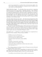
The flow and thermodynamics either in cylindrical nozzles or in Laval nozzles
can be completely described with commercially available numerical simulation pro-
grams, which an example of is presented in Fig. 3.16a. In that example, the pro-
gresses of Mach number, air density, air pressure and air temperature along the
nozzle length are completely documented. It can be seen that pressure, density and
temperature of the air are all reduced during the flow of the air through the nozzle.
The flow regimes that are set up in a convergent–divergent nozzle are best illus-
trated by considering the pressure decay in a given nozzle as the ambient (back)
pressure is reduced from rather high to very low values. All the operating modes
from wholly subsonic to underexpanded supersonic are shown in sequences “1” to
“5” in Fig. 3.26, which will be discussed later in Sect. 3.4.3.
3.2.5 Power, Impulse Flow and Temperature
The power of the air stream exiting a nozzle is simply given as follows:
P

A
=
˙m
A
2
· v
2
A
(3.24)
3.2 Air Flow in Nozzles 71
(a)
2
1
5
3
4
(b)
Fig. 3.16 Results of numerical simulations of the air flow in convergent–divergent nozzles (Laval
nozzles). (a) Gradients for Mach number (1), pressure (2), density (3), temperature (4) and air
velocity (5): image: RWTH Aachen, Aachen, (Germany); (b) Complete numerical nozzle design
including shock front computation (Aerorocket Inc., Citrus Springs, USA)
72 3 Air and Abrasive Acceleration
For the above-mentioned example, the air stream power is about P
A
= 16 kW.
The impulse flow of an air stream exiting a nozzle can be calculated as follows:
˙
I
A
= ˙m

A
· v
A
(3.25)
For the parameter combination mentioned above, the impulse flow is about
˙
I
A
= 65 N.
Because of the air expansion, air temperature drops over the nozzle length
(see Fig. 3.16a). The temperature of the air at the nozzle exit can be calculated
based on (3.19). A manipulation of this equation delivers the following relationship
(Bohl, 1989):
T
E
= T
N
−
v
2
A
2 · c
P
(3.26)
In that equation, T
N
is the entry temperature of the air. The value for the isobaric
heat capacity of air is listed in Table 3.1. For the above-mentioned example, (3.26)
delivers an air exit temperature of T
E

= 180 K (θ
E
=−93
◦
C).
3.3 Abrasive Particle Acceleration in Nozzles
3.3.1 General Aspects
Solid abrasives particles hit by an air stream do accelerate because of the drag force
imposed by the air stream. The situation is illustrated in Fig. 3.17 where results
of a numerical simulation of pressure contours and air streamlines around a sphere
are shown. The acceleration of the sphere is governed by Newton’s second law of
motion:
m
P
·
dv
P
dt
= F
D
= c
D
· A
P
·
ρ
A
2
·
|

v
A
− v
P0
|
2
(3.27)
The drag force F
D
depends on the particle drag coefficient, the average cross-
sectional area of the particle, the density of the air and on the relative velocity
between air and particle. The term |v
A
− v
P0
|=v
rel
is the relative velocity between
gas flow and particle flow. For very low particles flow velocities, for example, in the
entry section of a nozzle, v
rel
= v
A
.Theterm
1
/
2
· ρ
A
· v

2
rel
is equal to the dynamic
pressure of the air flow.
The drag coefficient is usually unknown and should be measured. It depends on
Reynolds number and Mach number of the flow: c
D
= f (Re, Ma), whereby the
Mach number is important if the air flow is compressible. Settles and Geppert (1997)
provided some results of measurements performed on particles at supersonic speeds.
3.3 Abrasive Particle Acceleration in Nozzles 73
Fig. 3.17 Numerically simulated pressure contours and flow streamlines on a solid particle in a
high-speed air flow (image: H.A. Dwyer, University of California, Davis)
Their results, plotted in Fig. 3.18, suggest that the drag coefficient only weakly de-
pends on Reynolds number,but is very sensitive to changes in the Mach number.The
c
D
-value is rather low at low Mach number values, but it dramatically increases after
a value of Ma = 1. It finally levels off around a value of unity for Mach numbers
greater than Ma = 1.4. More information on this issue is delivered by Bailey and
Hiatt (1972), who published c
D
–Ma–Re data for different nozzle geometries, and
by Fokke (1999). Other notable effects on the drag coefficient are basically those
1.2
1.0
0.8
0.6
0.4
0 0.5 1

Mach number
Re
= 2,000
Re = 20,000
C
D
value
1.5 2
Fig. 3.18 Effects of Mach number and Reynolds number on friction parameter (Settles and
Geppert, 1997)
74 3 Air and Abrasive Acceleration
of acceleration, of particle shape and of particle shielding, which are discussed in
Brauer’s (1971) book.
The air density is, in the first place, a function of pressure and temperature
as expressed by (3.6). This is an interesting point because both parameters no-
tably vary over the nozzle length as witnessed by the results of numerical sim-
ulations provided in Fig. 3.16a. Both air pressure and air temperature drop if
they approach the exit. The relative velocity can, for practical purposes, be re-
placed by the velocity of the air flow (v
A
 v
P0
), if the acceleration process
starts. In cylindrical nozzles, this velocity cannot exceed the speed of sound (see
Sect. 3.2). However, because speed of sound depends on gas temperature (3.9), a
theoretical possibility for an increase in drag force due to gas temperature increase
exists.
The acceleration acting on a particle during the particle–air interaction can be
approximated as follows:
a

P
= ˙v
P
=
F
D
m
P
(3.28)
This condition delivers the following relationship:
˙v
P
∝
c
D
· ρ
A
· v
2
A
d
P
· ρ
P
(3.29)
Acceleration values for convergent–divergent nozzles were calculated by
Achtsnick (2005), who estimated values as high as a
P
= 10
7

m/s
2
. This author could
also verify the trend expressed in (3.29) for the particle diameter. The particle accel-
eration increased extraordinarily when the abrasive particle diameter was reduced
below d
P
= 10 μm. If particles get smaller, they start to follow the trajectories of air
flow they are suspended, and the slip between particles and air flow reduces. The ac-
celeration period required to realise a given final particle speed can be approximated
as follows:
t
a
∝
v
P
· d
P
· ρ
P
c
D
· ρ
A
· v
2
A
(3.30)
Acceleration is, of course, not a constant value over the nozzle length, but (3.29)
depicts that acceleration effects are, in general, less severe if particles with larger

diameter and larger density are entrained into the air flow. For a desired particle
speed, acceleration period (nozzle length) must be increased if heavy (ρ
P
), respec-
tively large (d
P
), abrasive particles are injected. Acceleration period (nozzle length)
can be reduced if air flow density (ρ
A
), air flow velocity (v
A
) and drag coefficient
(c
D
) feature high values.
Equation (3.27) must be solved by numerical methods, and numerous authors
(Kamzolov et al., 1971; Ninham and Hutchings, 1983; Settles and Garg, 1995;
Settles and Geppert, 1997; Johnston, 1998; Fokke, 1999; Achtsnick et al., 2005)
utilised such methods and delivered appropriate solutions. Results of such calcula-
tion procedures are provided in the following sections.
3.3 Abrasive Particle Acceleration in Nozzles 75
3.3.2 Simplified Solution
Iida (1996) and Kirk (2007) provided an approximation for the velocity of parti-
cles accelerated in a cylindrical blast cleaning nozzle. The solution of Iida (1996)
neglects effects of friction parameter and air density. Kirk’s (2007) approximation
reads as follows:

v
P
v

A
− v
P

2
=
c
D
· L
N
d
P
·
ρ
A
ρ
P
(3.31)
Due to certain simplifications, this equation can only serve for the assessment of
trends, but cannot deliver suitable quantitative results. A solution to (3.31) delivers
the following trends:
v
P
∝ p
0.68
(3.32a)
v
P
∝ d
−0.36

P
(3.32b)
v
P
∝ ρ
−0.38
P
(3.32c)
Uferer (1992) applied a simplified numerical procedure for the calculation of
abrasive particles accelerated in blast cleaning nozzles. Some results of these cal-
culations for two nozzle layouts are provided in Fig. 3.19. The graphs demonstrate
that the utilisation of a Laval nozzle increases the velocities of air and abrasive
particles, but the gain is much higher for the air acceleration. The reason is the
drop in air density in the divergent section of the Laval nozzle (see Fig. 3.16a).
According to (3.27), this causes a reduction in the drag force acting at the particles
to be accelerated. Thus, although Laval nozzles are very efficient in air acceleration,
they do not increase the abrasive exit speed at an equally high ratio.
3.3.3 Abrasive Flux Rate
The abrasive flux rate through a nozzle (in kg/s per unit nozzle area passing through
the nozzle) can be approximated as follows (Ciampini et al., 2003b):
˙m
N
= ρ
P
· v
P
· ρ
∗
S
(3.33)

Thus, for a given abrasive material and incident abrasive velocity, interference
effects resulting from changes in flux are described by the dimensionless stream
density (see Sect. 3.5.5).
76 3 Air and Abrasive Acceleration
Fig. 3.19 Effects of nozzle layout on calculated air and abrasive velocities (Uferer, 1993)
3.3.4 Abrasive Particle Spacing
The average distance between individual abrasive particles in a blast cleaning nozzle
can be approximated as follows (Shipway and Hutchings, 1994):
L
P
=

m
P
· v
P
· π ·r
2
N
˙m
P

1/3
(3.34)
Results obtained by Shipway and Hutchings (1994) are listed in Table 3.5. The
ratio between spacing distance and abrasive particle diameter had a typical value
of about L
P
/d
P

= 15. For a low abrasive mass flow rate, this value increased up to
L
P
/d
P
= 23.
Table 3.5 Average distances between abrasive particles in a blast cleaning nozzle (Shipway and
Hutchings, 1994)
Particle diameter in Particle velocity Abrasive mass flow Average distance L
P
/d
P
μm in m/s rate in g/min in μm
63–75 70 50 900 ∼ 13
125–150 52 6 3,200 ∼ 23
212–250 45 31 4,000 ∼ 17
650–750 29 37 7,900 ∼ 13
3.4 Jet Structure 77
3.4 Jet Structure
3.4.1 Structure of High-speed Air Jets
A schematicsketch ofa freeair jetis shown inFig. 3.20.The term “free jet” designates
systems where a fluid issues from a nozzle into a stagnant medium, which consists
of the same medium as the jet. Two main regions can be distinguished in the jet: an
initial region and a main region. The initial region is characterisedbya potential core,
which has an almost uniform mean velocity equal to the exit velocity. The velocity
profile is smooth in that region. Due to the velocity difference between the jet and
the ambient air, a thin shear layer forms. This layer is unstable and is subjected to
flow instabilities that eventually lead to the formation of vertical structures. Because
of the spreading of the shear layer, the potential core disappears at a certain stand-off
distance. Ambient air entrains thejet, and entrainment and mixing processes continue

beyondthe end ofthe potentialcore.In themain region, the radial velocity distribution
in the jet finally changes to a pronounced bell-shaped velocity profile as illustrated in
Fig. 3.20.The angle θ
J
is theexpansion angle of the jet. In order to calculatethis angle,
the border between air jet and surrounding air flow must be defined. One definition is
the half-width of the jet defined as the distance between the jet axis and the location
where the local velocity [v
J
(x,r)] is equal to the half of the local maximum velocity
situated on the centreline [v
J
(x,r =0)]. Achtsnick (2005)who applied this definition
estimated typical expansion angles between θ
J
= 12.5
◦
and 15
◦
.
Shipway and Hutchings (1993a) took schlieren images from acetone-air plumes
exiting cylindrical steel nozzles at rather low air pressures up to p = 0.09 MPa,
and they could prove that the plume shape differed just insignificantly if the gas
exited either from a nozzle with a low internal roughness (R
a
= 0.25 μm) or from
a nozzle with a rough wall structure (R
a
= 0.94 μm). This situation changed if
abrasive particles were added to the air flow.

The structure of an abrasive jet is disturbed due to rebounding abrasive parti-
cles if the nozzle is being brought very close to the specimen surface. This was
mixing zone
surroundings
jet cross-section
main region
core region
nozzle
d
N
v
A
θ
J
Fig. 3.20 Structure of an air jet issued from a nozzle into stagnant air (adapted from Achtsnick,
2005)
78 3 Air and Abrasive Acceleration
verified by Shipway and Hutchings (1994) who took long-exposure photographs of
the trajectories of glass spheres in an air jet and observed many particle trajectories,
which deviated strongly from the nozzle axis. It was supposed that these are particles
rebounding from the target.
3.4.2 Structure of Air-particle Jets
Plaster (1972) was probably the first who advised the blast cleaning industry into
the effect of nozzle configuration on the structure of air-particle jets. The images
shown in Fig. 3.21 clearly illustrate the influence of nozzle design on jet stability.
Figure 3.21a shows a jet exiting from a badly designed nozzle, which results in a
shock wave at the tip (central image) and in an erratic projection of abrasives (right
image). A correctly designed nozzle is shown in Fig. 3.21b. This nozzle produces
a smooth flow as can be seen by the configuration of the air stream (central image)
and by the even projection of the abrasives (right image).

The width (radius) of high-speed air-particle jets at different jet lengths was
measured by Fokke (1999) and Slikkerveer (1999). Kirk and Abyaneh (1994) and
Slikkerveer (1999) provided an empirical relationship as follows:
(a)
(b)
Fig. 3.21 Effect of nozzle design on jet structure and abrasive acceleration (Plaster, 1972).
(a) Badly designed nozzle; (b) Correctly designed nozzle
3.4 Jet Structure 79
d
J
= d
N
+ 2 · x · tan θ
J
(3.35)
The expansion angle can be considered to be between θ
J
=3
◦
and 7
◦
(Slikkerveer,
1999; Achtsnick et al., 2005). Therefore, it is smaller than for a plain air jet. Results
of calculations based on (3.35) for θ
J
=5
◦
are displayed in Fig. 3.22.
Fokke (1999) found an almost linear relationship between jet half width and jet
length. The air mass flow rate showed marginal effects on the half width at longer

jet lengths: with an increase in air mass flow rate, half width slightly decreased.
Some relationships are illustrated in Fig. 3.23. These results corresponded to that of
Mellali et al. (1994) who found a linear relationship between stand-off distance and
the area of the cross-section hit by a blast cleaning jet.
Shipway and Hutchings (1993a) took schlieren images from glass bead plumes
exiting cylindrical steel nozzles at air pressures up to p = 0.09 MPa. They noted
a distinct effect of the nozzle wall roughness on the plume shape as a result
of the differences in the interaction of the particles with the nozzle wall. Vari-
ations in the rebound behaviour of the glass beads on impact with the nozzle
wall caused the particles to leave the nozzle exit with different angular distribu-
tions. These authors also defined a “plume spread parameter”, respectively a “focus
coefficient”:
β
P
= α
P
· x (3.36)
12
9
6
3
0
01020
stand-off distance in mm
d
N
= 6 mm
d
N
= 8 mm

d
N
= 12 mm
jet radius in mm
30
Fig. 3.22 Radius of a particle-air jet according to (3.35)