Computational Physics - M. Jensen Episode 1 Part 4 pdf
Bạn đang xem bản rút gọn của tài liệu. Xem và tải ngay bản đầy đủ của tài liệu tại đây (276.56 KB, 20 trang )
3.2. NUMERICAL DIFFERENTIATION 49
computed_d eri vati ve = new double [ number_of_steps ] ;
/ / compute the second d e r i v a t i v e of exp ( x )
se c o n d _ d e r i v a t i v e ( number_of_steps , x , i n i t i a l _ s t e p , h_step ,
computed_d er ivat ive ) ;
/ / Then we p r i n t the r e s u l t s to f i l e
out pu t ( h_step , computed_derivative , x , number_of_steps ) ;
/ / f r e e memory
de le te [ ] h_step ;
de le te [ ] computed_de riv at ive ;
return 0 ;
} / / end main program
We have defined three additional functions, one which reads in from screen the value of , the
initial step length
and the number of divisions by 2 of . This function is called initialise .
To calculate the second derivatives we define the function second_derivative . Finally, we have a
function which writes our results together with a comparison with the exact value to a given file.
The results are stored in two arrays, one which contains the given step length
and another one
which contains the computed derivative.
These arrays are defined as pointers through the statement
double h_step , computed_derivative
; A call in the main function to the function second_derivative looks then like this second_derivative
( number_of_steps , x , h_step , computed_derivative ); while the called function is declared in the
following way void second_derivative (int number_of_steps , double x , double h_step,double computed_derivati
); indicating that double h_step , double computed_derivative ; are pointers and that we transfer
the address of the first elements. The other variables
int number_of_steps, double x; are trans-
ferred by value and are not changed in the called function.
Another aspect to observe is the possibility of dynamical allocation of memory through the
new function. In the included program we reserve space in memory for these three arrays in
the following way h_step = new double[number_of_steps]; and computed_derivative = new double
[number_of_steps]; When we no longer need the space occupied by these arrays, we free memory
through the declarations delete [] h_step; and delete [] computed_derivative ;
The function initialise
/ / Read in from screen the i n i t i a l step , the number of st e ps
/ / and the value of x
void i n i t i a l i s e ( double i n i t i a l _ s t e p , double x , in t
number_of_steps )
{
p r i n t f ( )
;
scanf ( , i n i t i a l _ s t e p , x , number_of_steps ) ;
return ;
} / / end of f u n ct i on i n i t i a l i s e
50 CHAPTER 3. NUMERICAL DIFFERENTIATION
This function receives the addresses of the three variables double initial_step , double x
, int number_of_steps; and returns updated values by reading from screen.
The function second_derivative
/ / This f un ct i on computes the second d e r i v a t i v e
void se c o n d _ d e r i v a t i v e ( int number_of_steps , double x ,
double i n i t i a l _ s t e p , double h_step ,
double computed_d eri vati ve )
{
in t count er ;
double y , d er i v at i v e , h ;
/ / c a lc ul at e the s te p s i z e
/ / i n i t i a l i s e the de r i v at i v e , y and x ( i n minutes )
/ / and i t e r a t i o n counter
h = i n i t i a l _ s t e p ;
/ / s t a r t computing f or d i f f e r e n t s te p s i z e s
for ( co unt er = 0 ; cou nt er < number_of_steps ; c ou nt er ++ )
{
/ / setup arrays with d e r i v a t i v e s and st ep s i z e s
h_step [ co un te r ] = h ;
computed_d eri vati ve [ co un te r ] =
( exp ( x+h ) 2. exp ( x )+exp (x h ) ) / ( h h) ;
h = h 0 . 5 ;
} / / end of do loop
return ;
} / / end of f u n c ti o n second d e r i v a t i v e
The loop over the number of steps serves to compute the second derivative for different values
of . In this function the step is halved for every iteration. The step values and the derivatives
are stored in the arrays h_step and double computed_derivative.
The output function
This function computes the relative error and writes to a chosen file the results.
/ / f u n c ti o n to wri te out the f i n a l r e s u l t s
void outp ut ( double h_step , double computed_derivative , double x ,
in t number_of_steps )
{
in t i ;
FILE o u t p u t _ f i l e ;
o u t p u t _ f i l e = fopen ( , ) ;
for ( i =0 ; i < number_of_steps ; i ++)
{
3.2. NUMERICAL DIFFERENTIATION 51
f p r i n t f ( o u tp u t_ fi l e , ,
log10 ( h_step [ i ] ) ,
log10 ( fabs ( computed_ der iv ati ve [ i ] exp ( x ) ) / exp ( x ) ) ) ;
}
f c lo se ( o u t p u t _ f i l e ) ;
} / / end of f u n ct i on outp ut
The last function here illustrates how to open a file, write and read possible data and then close it.
In this case we have fixed the name of file. Another possibility is obviously to read the name of
this file together with other input parameters. The way the program is presented here is slightly
unpractical since we need to recompile the program if we wish to change the name of the output
file.
An alternative is represented by the following program. This program reads from screen the
names of the input and output files.
1 # inclu de < st d i o . h>
2 # inclu de < s t d l i b . h>
3 int col :
4
5 int main ( in t argc , char argv [ ] )
6 {
7 FILE in , out ;
8 in t c ;
9 i f ( argc < 3) {
10 p r i n t f ( ) ;
11 p r i n t f ( ) ;
12 ex i t ( 0) ;
13 in = fopen ( argv [ 1 ] , ) ; } / / re t u r n s p o i nt e r to the i n _ f i l e
14 i f ( inn == NULL ) { / / can ’ t fi nd i n _ f i l e
15 p r i n t f ( , argv [ 1 ] ) ;
16 ex i t ( 0) ;
17 }
18 out = fopen ( argv [ 2 ] , ) ; / / re t u r n s a p o i nt e r to the
o u t _ f i l e
19 i f ( ut == NULL ) { / / can ’ t f i n d o u t _ f i l e
20 p r i n t f ( , argv [ 2 ] ) ;
21 ex i t ( 0) ;
22 }
. . . program s t a t e m e n t s
23 fc l o s e ( in ) ;
24 fc l o s e ( out ) ;
25 return 0 ;
}
This program has several interesting features.
52 CHAPTER 3. NUMERICAL DIFFERENTIATION
Line Program comments
5 takes three arguments, given by argc. argv points to the fol-
lowing: the name of the program, the first and second arguments, in
this case file names to be read from screen. kommandoen.
7 C/C++ has a called . The pointers and point
to specific files. They must be of the type
.
10 The command line has to contain 2 filenames as parameters.
13–17 The input files has to exit, else the pointer returns NULL. It has only
read permission.
18–22 Same for the output file, but now with write permission only.
23–24 Both files are closed before the main program ends.
The above represents a standard procedure in C for reading file names. C++ has its own class
for such operations. We will come back to such features later.
Results
In Table 3.1 we present the results of a numerical evaluation for various step sizes for the second
derivative of
using the approximation . The results are compared with
the exact ones for various
values. Note well that as the step is decreased we get closer to the
Exact
0.0 1.000834 1.000008 1.000000 1.000000 1.010303 1.000000
1.0 2.720548 2.718304 2.718282 2.718282 2.753353 2.718282
2.0 7.395216 7.389118 7.389057 7.389056 7.283063 7.389056
3.0 20.102280 20.085704 20.085539 20.085537 20.250467 20.085537
4.0 54.643664 54.598605 54.598155 54.598151 54.711789 54.598150
5.0 148.536878 148.414396 148.413172 148.413161 150.635056 148.413159
Table 3.1: Result for numerically calculated second derivatives of . A comparison is
made with the exact value. The step size is also listed.
exact value. However, if it is further decreased, we run into problems of loss of precision. This
is clearly seen for
. This means that even though we could let the computer run
with smaller and smaller values of the step, there is a limit for how small the step can be made
before we loose precision.
3.2.2 Error analysis
Let us analyze these results in order to see whether we can find a minimal step length which does
not lead to loss of precision. Furthermore In Fig. 3.2 we have plotted
(3.28)
3.2. NUMERICAL DIFFERENTIATION 53
Relative error
log
0
-2-4
-6-8-10
-12-14
6
4
2
0
-2
-4
-6
-8
-10
Figure 3.2: Log-log plot of the relative error of the second derivative of
as function of decreas-
ing step lengths . The second derivative was computed for in the program discussed
above. See text for further details
as function of
. We used an intial step length of and fixed . For large
values of , that is we see a straight line with a slope close to 2. Close to
the relative error starts increasing and our computed derivative with a step size
, may no longer be reliable.
Can we understand this behavior in terms of the discussion from the previous chapter? In
chapter 2 we assumed that the total error could be approximated with one term arising from the
loss of numerical precision and another due to the truncation or approximation made, that is
(3.29)
For the computed second derivative, Eq. (3.15), we have
and the truncation or approximation error goes like
If we were not to worry about loss of precision, we could in principle make as small as possible.
However, due to the computed expression in the above program example
54 CHAPTER 3. NUMERICAL DIFFERENTIATION
we reach fairly quickly a limit for where loss of precision due to the subtraction of two nearly
equal numbers becomes crucial. If
are very close, we have , where
for single and for double precision, respectively.
We have then
Our total error becomes
(3.30)
It is then natural to ask which value of
yields the smallest total error. Taking the derivative of
with respect to results in
(3.31)
With double precision and
we obtain
(3.32)
Beyond this value, it is essentially the loss of numerical precision which takes over. We note
also that the above qualitative argument agrees seemingly well with the results plotted in Fig.
3.2 and Table 3.1. The turning point for the relative error at approximately
reflects
most likely the point where roundoff errors take over. If we had used single precision, we would
get
. Due to the subtractive cancellation in the expression for there is a pronounced
detoriation in accuracy as is made smaller and smaller.
It is instructive in this analysis to rewrite the numerator of the computed derivative as
as
since it is the difference which causes the loss of precision. The results, still
for are shown in the Table 3.2. We note from this table that at we have
essentially lost all leading digits.
From Fig. 3.2 we can read off the slope of the curve and thereby determine empirically how
truncation errors and roundoff errors propagate. We saw that for
, we could
extract a slope close to
, in agreement with the mathematical expression for the truncation error.
We can repeat this for and extract a slope . This agrees again
with our simple expression in Eq. (3.30).
3.2.3 How to make figures with Gnuplot
Gnuplot is a simple plotting program which follows the Linux/Unix operating system. It is easy
to use and allows also to generate figure files which can be included in a L
A
T
E
X document. Here
3.2. NUMERICAL DIFFERENTIATION 55
2.0100083361116070 1.0008336111607230
2.0001000008333358 1.0000083333605581
2.0000010000000836 1.0000000834065048
2.0000000099999999 1.0000000050247593
2.0000000001000000 9.9999897251734637
2.0000000000010001 9.9997787827987850
2.0000000000000098 9.9920072216264089
2.0000000000000000 0.0000000000000000
2.0000000000000000 1.1102230246251565
2.0000000000000000 0.0000000000000000
Table 3.2: Result for the numerically calculated numerator of the second derivative as function
of the step size . The calculations have been made with double precision.
we show how to make simple plots online and how to make postscript versions of the plot or
even a figure file which can be included in a L
A
T
E
X document. There are other plotting programs
such as xmgrace as well which follow Linux or Unix as operating systems.
In order to check if gnuplot is present type
If gnuplot is available, simply write
to start the program. You will then see the following prompt
and type help for a list of various commands and help options. Suppose you wish to plot data
points stored in the file mydata.dat. This file contains two columns of data points, where the
first column refers to the argument
while the second one refers to a computed function value
.
If we wish to plot these sets of points with gnuplot we just to need to write
or
since gnuplot assigns as default the first column as the -axis. The abbreviations w l stand for
’with lines’. If you prefer to plot the data points only, write
56 CHAPTER 3. NUMERICAL DIFFERENTIATION
For more plotting options, how to make axis labels etc, type help and choose plot as topic.
Gnuplot will typically display a graph on the screen. If we wish to save this graph as a
postscript file, we can proceed as follows
and you will be the owner of a postscript file called mydata.ps, which you can display with
ghostview through the call
The other alternative is to generate a figure file for the document handling program L
A
T
E
X.
The advantage here is that the text of your figure now has the same fonts as the remaining L
A
T
E
X
document. Fig. 3.2 was generated following the steps below. You need to edit a file which ends
with .gnu. The file used to generate Fig. 3.2 is called derivative.gnu and contains the following
statements, which are a mix of L
A
T
E
X and Gnuplot statements. It generates a file derivative.tex
which can be included in a L
A
T
E
X document.
To generate the file derivative.tex, you need to call Gnuplot as follows
You can then include this file in a L
A
T
E
X document as shown here
3.3. RICHARDSON’S DEFERRED EXTRAPOLATION METHOD 57
3.3 Richardson’s deferred extrapolation method
Here we will show how one can use the polynomial representation discussed above in order to im-
prove calculational results. We will again study the evaluation of the first and second derivatives
of
at a given point . In Eqs. (3.14) and (3.15) for the first and second derivatives,
we noted that the truncation error goes like
.
Employing the mid-point approximation to the derivative, the various derivatives
of a given
function
can then be written as
(3.33)
where
is the calculated derivative, the exact value in the limit and are
independent of . By choosing smaller and smaller values for , we should in principle be
able to approach the exact value. However, since the derivatives involve differences, we may
easily loose numerical precision as shown in the previous sections. A possible cure is to apply
Richardson’s deferred approach, i.e., we perform calculations with several values of the step
and extrapolate to . The philososphy is to combine different values of so that the terms
in the above equation involve only large exponents for . To see this, assume that we mount a
calculation for two values of the step , one with and the other with . Then we have
(3.34)
and
(3.35)
and we can eliminate the term with
by combining
(3.36)
We see that this approximation to
is better than the two previous ones since the error now
goes like
. As an example, let us evaluate the first derivative of a function using a step
with lengths and . We have then
(3.37)
(3.38)
which can be combined, using Eq. (3.36) to yield
(3.39)
58 CHAPTER 3. NUMERICAL DIFFERENTIATION
In practice, what happens is that our approximations to goes through a series of steps
(3.40)
where the elements in the first column represent the given approximations
(3.41)
This means that
in the second column and row is the result of the extrapolating based on
and . An element in the table is then given by
(3.42)
with
. I.e., it is a linear combination of the element to the left of it and the element right
over the latter.
In Table 3.1 we presented the results for various step sizes for the second derivative of
using . The results were compared with the exact ones for various values.
Note well that as the step is decreased we get closer to the exact value. However, if it is further
increased, we run into problems of loss of precision. This is clearly seen for . This
means that even though we could let the computer run with smaller and smaller values of the
step, there is a limit for how small the step can be made before we loose precision. Consider
now the results in Table 3.3 where we choose to employ Richardson’s extrapolation scheme. In
this calculation we have computed our function with only three possible values for the step size,
namely
, and with . The agreement with the exact value is amazing! The
extrapolated result is based upon the use of Eq. (3.42).
Extrapolat Error
0.0 1.00083361 1.00020835 1.00005208 1.00000000 0.00000000
1.0 2.72054782 2.71884818 2.71842341 2.71828183 0.00000001
2.0 7.39521570 7.39059561 7.38944095 7.38905610 0.00000003
3.0 20.10228045 20.08972176 20.08658307 20.08553692 0.00000009
4.0 54.64366366 54.60952560 54.60099375 54.59815003 0.00000024
5.0 148.53687797 148.44408109 148.42088912 148.41315910 0.00000064
Table 3.3: Result for numerically calculated second derivatives of using extrapolation.
The first three values are those calculated with three different step sizes, , and with
. The extrapolated result to should then be compared with the exact ones from
Table 3.1.
Chapter 4
Classes, templates and modules
in preparation (not finished as of 11/26/03)
4.1 Introduction
C++’ strength over C and F77 is the possibility to define new data types, tailored to some prob-
lem.
A user-defined data type contains data (variables) and functions operating on the data
Example: a point in 2D
– data: x and y coordinates of the point
– functions: print, distance to another point,
Classes into structures
Pass arguments to methods
Allocate storage for objects
Implement associations
Encapsulate internal details into classes
Implement inheritance in data structures
Classes contain a new data type and the procedures that can be performed by the class. The
elements (or components) of the data type are the class data members, and the procedures are the
class member functions.
61
62 CHAPTER 4. CLASSES, TEMPLATES AND MODULES
4.2 A first encounter, the vector class
Class MyVector: a vector
Data: plain C array
Functions: subscripting, change length, assignment to another vector, inner product with
another vector,
This examples demonstrates many aspects of C++ programming
Create vectors of a specified length: MyVector v(n);
Create a vector with zero length: MyVector v;
Redimension a vector to length n: v.redim(n);
Create a vector as a copy of another vector w: MyVector v(w);
Extract the length of the vector: const int n = v.size();
Extract an entry: double e = v(i);
Assign a number to an entry: v(j) = e;
Set two vectors equal to each other: w = v;
Take the inner product of two vectors: double a = w.inner(v);
or alternatively a = inner(w,v);
Write a vector to the screen: v.print(cout);
c l a s s MyVector
{
private :
double A; / / vect or e n t r i e s ( C array )
in t l en gt h ;
void a l l o c a t e ( i nt n ) ; // a l l o c a te memory , leng th =n
void de a l l o c at e ( ) ; / / f r e e memory
public :
MyVector ( ) ; / / MyVector v ;
MyVector ( i n t n ) ; / / MyVector v ( n ) ;
MyVector ( const MyVector & w) ; / / MyVector v (w) ;
~MyVector ( ) ; / / clean up dynamic memory
bool redim ( in t n ) ; / / v . redim (m) ;
MyVector & operator = ( const MyVector& w) ; / / v = w;
4.2. A FIRST ENCOUNTER, THE VECTOR CLASS 63
double operator ( ) ( int i ) const ; / / a = v ( i ) ;
double & operator ( ) ( i n t i ) ; / / v ( i ) = a ;
void p r i n t ( std : : ostream & o ) const ; / / v . pr i n t ( cout ) ;
double i nn er ( const MyVector& w) const ; / / a = v . inner (w) ;
in t s i z e ( ) const { return leng th ; } / / n = v . s i ze ( ) ;
};
\ end { l i s t i n g }
C o n s t r u c t o r s t e l l how we de c l a r e a v a r i a b l e of type MyVector and how
t h i s va r i a b l e i s i n i t i a l i z e d
\ begin { l s t l i s t i n g }
MyVector v ; / / dec la re a ve ct or of len gt h 0
/ / t h i s a c tu a l l y means c a l l i n g the fu nc ti o n
MyVector : : MyVector ( )
{ A = NULL ; l en gt h = 0 ; }
MyVector v( n ) ; / / dec la re a vec to r of len gt h n
/ / means c a l l i n g the f u n c ti o n
MyVector : : MyVector ( in t n )
{ a l l o c a t e ( n ) ; }
void MyVector : : a l l o c a t e ( int n )
{
le ngt h = n ;
A = new double [ n ] ; / / cre at e n doubles in memory
}
A MyVector object is created (dynamically) at run time, but must also be destroyed when it
is no longer in use. The destructor specifies how to destroy the object:
MyVector :: ~ MyVector ( )
{
d e al l o ca t e ( ) ;
}
/ / f r e e dynamic memory :
void MyVector : : d e al l o ca t e ( )
{
de le te [ ] A;
}
64 CHAPTER 4. CLASSES, TEMPLATES AND MODULES
/ / v and w are MyVector o b je ct s
v = w;
/ / means c a l l i n g
MyVector & MyVector : : operator = ( const MyVector & w)
/ / for s e t t i n g v = w;
{
redim (w. s i ze () ) ; / / make v as long as w
in t i ;
for ( i = 0 ; i < l en gt h ; i ++) { / / ( C arrays s t a r t at 0)
A[ i ] = w.A[ i ] ;
}
return t hi s ;
}
/ / ret u rn of this , i . e . a MyVector & , allows nes te d
u = v = u_vec = v_vec ;
v . redim ( n ) ; / / make a v of le ng th n
bool MyVector : : redim ( in t n )
{
i f ( l en gt h = = n )
return f a l s e ; / / no need to a l l o c a t e anything
el s e {
i f (A ! = NULL) {
/ / " t h i s " ob j e ct has already al l o c at e d memory
d e al l o c a t e ( ) ;
}
a l l o c a t e ( n ) ;
return true ; / / the le ng t h was changed
}
}
MyVector v(w) ; / / take a copy of w
MyVector : : MyVector ( const MyVector& w)
{
a l l o c a t e (w. s i ze ( ) ) ; / / " t h i s " obj e c t ge ts w ’ s le ng th
t h i s = w ; / / c a l l operator=
}
/ / a and v are MyVector o bj ec t s ; want to s et
a ( j ) = v ( i +1) ;
4.2. A FIRST ENCOUNTER, THE VECTOR CLASS 65
/ / the meaning of a ( j ) is def in ed by
i n l in e double& MyVector : : operator ( ) ( i nt i )
{
return A[ i 1];
/ / base index i s 1 ( not 0 as in C/C++)
}
Inline functions: function body is copied to calling code, no overhead of function call!
Note: inline is just a hint to the compiler; there is no guarantee that the compiler really
inlines the function
Why return a double reference?
double & MyVector : : operator ( ) ( int i ) { return A[ i 1]; }
/ / re t u r n s a re f e r e n c e ( ‘ ‘ po i n t e r ’ ’) d i r e c t l y to A[ i 1]
/ / such th at the c a l l i n g code can change A[ i 1]
/ / given MyVector a ( n ) , b ( n ) , c ( n ) ;
for ( i nt i = 1 ; i <= n ; i ++)
c ( i ) = a ( i ) b ( i ) ;
/ / com piler i n l i n i n g t r a n s l a t e s t h i s to :
for ( i nt i = 1 ; i <= n ; i ++)
c .A[ i 1] = a .A[ i 1] b .A[ i 1];
/ / or perhaps
for ( i nt i = 0 ; i < n ; i ++)
c .A[ i ] = a .A[ i ] b .A[ i ] ;
/ / more o p ti m i z a ti on s by a smart compiler :
double ap = & a .A[ 0 ] ; / / s t a r t of a
double bp = &b .A [ 0 ] ; / / s t a r t of b
double cp = & c .A[ 0 ] ; / / s t a r t of c
for ( i nt i = 0 ; i < n ; i ++)
cp [ i ] = ap [ i ] bp [ i ] ; / / pure C!
Inlining and the programmer’s complete control with the definition of subscripting allow
void MyVector : : p r i n t ( s td : : ostream & o ) const
{
in t i ;
for ( i = 1 ; i <= len gt h ; i ++)
o < < < < i < < < < ( t hi s ) ( i ) < < ;
}
66 CHAPTER 4. CLASSES, TEMPLATES AND MODULES
double a = v . inn er (w) ;
double MyVector : : inn e r ( const MyVector& w) const
{
in t i ; double sum = 0 ;
for ( i = 0 ; i < leng th ; i ++)
sum += A[ i ] w.A[ i ] ;
/ / a l t e r n a t i v e :
/ / for ( i = 1 ; i <= lengt h ; i ++) sum += ( t h i s ) ( i ) w( i ) ;
return sum ;
}
/ / MyVector v
cout < < v ;
ostream & operator < < ( ostream & o , const MyVector & v )
{ v . p r i n t ( o ) ; return o ; }
/ / must ret ur n ostream & for nes te d out pu t op er ato rs :
cout < < < < w;
/ / t h i s i s re a l i z e d by th es e c a l l s :
operator < < ( cout , ) ;
operator < < ( cout , w) ;
We can redefine the multiplication operator to mean the inner product of two vectors:
double a = v w; / / example on a t t r a c t i v e syn tax
c l a s s MyVector
{
. . .
/ / compute ( t h i s ) w
double operator ( const MyVector& w) const ;
. . .
};
double MyVector : : operator ( const MyVector & w) const
{
return i nn er (w) ;
}
/ / have some MyVector u , v , w ; double a ;
u = v + a w;
/ / glob al fu n c ti o n operator+
MyVector operator + ( const MyVector & a , const MyVector& b)
{
4.3. CLASSES AND TEMPLATES IN C++ 67
MyVector tmp ( a . si ze ( ) ) ;
for ( int i = 1; i <=a . s iz e ( ) ; i ++)
tmp ( i ) = a ( i ) + b ( i ) ;
return tmp ;
}
/ / glob al fu n c ti o n operator
MyVector operator ( const MyVector & a , double r )
{
MyVector tmp ( a . si ze ( ) ) ;
for ( int i = 1; i <=a . s iz e ( ) ; i ++)
tmp ( i ) = a ( i ) r ;
return tmp ;
}
/ / symmetric operator : r a
MyVector operator ( double r , const MyVector& a )
{ return operator ( a , r ) ; }
4.3 Classes and templates in C++
Class MyVector is a vector of doubles
What about a vector of floats or ints?
Copy and edit code ?
No, this can be done automatically by use of macros or templates!!
Templates are the native C++ constructs for parameterizing parts of classes
template <typename Type>
c l a s s MyVector
{
Type A;
in t len gt h ;
public :
. . .
Type& operator () ( i n t i ) { return A[ i 1]; }
. . .
};
Declarations in user code:
MyVector <double > a (10) ;
MyVector <int > co un te rs ;
Much simpler to use than macros for parameterization.
68 CHAPTER 4. CLASSES, TEMPLATES AND MODULES
It is easy to use class MyVector
Lots of details visible in C and Fortran 77 codes are hidden inside the class
It is not easy to write class MyVector
Thus: rely on ready-made classes in C++ libraries unless you really want to write develop
your own code and you know what are doing
C++ programming is effective when you build your own high-level classes out of well-
tested lower-level classes
4.4 Using Blitz++ with vectors and matrices
4.5 Building new classes
4.6 MODULE and TYPE declarations in Fortran 90/95
4.7 Object orienting in Fortran 90/95
4.8 An example of use of classes in C++ and Modules in For-
tran 90/95