Báo cáo toán học: "A Combinatorial Approach to Evaluation of Reliability of the Receiver Output for BPSK Modulation with Spatial Diversit" pot
Bạn đang xem bản rút gọn của tài liệu. Xem và tải ngay bản đầy đủ của tài liệu tại đây (244.44 KB, 31 trang )
A Combinatorial Approach to Evaluation of
Reliability of the Receiver Output for BPSK
Modulation with Spatial Diversity
S. Bliudze D. Krob
{bliudze, dk}@lix.polytechnique.fr
LIX,
´
Ecole Polytechnique, Route de Saclay
91128 Palaiseau Cedex, France
Submitted: Jul 22, 2004; Accepted: Jan 3, 2006; Published: Jan 7, 2006
Mathematics Subject Classifications: 05E05, 05E10
Abstract
In the context of soft demodulation of a digital signal modulated with Binary Phase Shift
Keying (BPSK) technique and in presence of spatial diversity, we show how the theory
of symmetric functions can be used to compute the probability that the log-likelihood of
a recieved bit is less than a given threshold ε. We show how such computation can be
reduced to computing the probability that U − V<ε(denoted P (U −V<ε)) where U
and V are two real random variables such that U =
N
i=1
|u
i
|
2
and V =
N
i=1
|v
i
|
2
where
the u
i
’s and v
i
’s are independent centered complex Gaussian variables with variances
E[ |u
i
|
2
]=χ
i
and E[ |v
i
|
2
]=δ
i
. We give two expressions in terms of symmetric functions
over the alphabets ∆ = (δ
1
, ,δ
N
)andX =(χ
1
, ,χ
N
) for the first 2N −1coefficients
of the Taylor expansion of P (U −V<ε)intermsofε. The first one is a quotient of multi-
Schur functions involving two alphabets derived from alphabets ∆ and X, which allows
us to give an efficient algorithm for the computation of these coefficients. The second
expression involves a certain sum of pairs of Schur functions s
λ
(∆) and s
µ
(X)whereλ
and µ are complementary shapes inside a N × N rectangle. We show that such a sum
has a natural combinatorial interpretation in terms of what we call square tabloids with
ribbons and that there is a natural extension of the Knuth correspondence that associates
a (0,1)-matrix to each square tabloid with ribbon. We then show that we can completely
characterise the (0,1)-matrices that arise from square tabloids with ribbons under this
correspondence.
the electronic journal of combinatorics 13 (2006), #R2 1
1 Introduction
In this paper we show how combinatorial techniques, such as symmetric functions and
the theory of Young tableaux, arise naturally in a rather applied context of digital com-
munications. Let us, therefore, start by introducing the reader to some aspects of the
latter.
Modulating numerical signals means transforming them into wave forms. Due to their
importance in practice, modulation methods were widely studied in signal processing
(see, for instance, chapter 5 of [18]). One of the most important problems in this area is
the performance evaluation of the optimum receivers associated with a given modulation
method, which leads to the computation of various probabilities of errors (see again [18]).
Among the different modulation protocols used in practical contexts, an important
class consists of methods where the modulation reference (i.e. a fixed numerical sequence)
is transmitted on the same channel as the usual signal. The demodulation decision is then
based on at least two noisy signals, namely, the transmitted signal and the transmitted
reference. It happens, however, that one can also take into account in the demodulation
process several noisy copies of these two signals: one speaks then of demodulation with
diversity. It appears that the probability of errors encountered in such contexts is of the
following form:
P (U<V)=P
U =
N
i=1
|u
i
|
2
<V=
N
i=1
|v
i
|
2
, (1)
where the u
i
and v
i
’s denote independent centered complex Gaussian random variables
with variances equal to
E[ |u
i
|
2
]=χ
i
and E[ |v
i
|
2
]=δ
i
for every i ∈ [1,N] (cf also Section
3.1).
The problem of computing explicitely probabilities of this last type was studied in
signal processing by several researchers (cf [2, 11, 18, 22]). The most interesting result in
this direction is due to Barett ([2]) who obtained the following expression
P (U<V)=
N
k=1
i=k
1
1 − δ
−1
k
δ
i
N
i=1
1
1+δ
−1
k
χ
i
,
for the probability given by formula (1).
In this paper, we consider the log-likelihood of a bit — the value of the so-called soft
bit obtained at the output of the rake receiver. This value allows one to decide what was
the value of the transmitted bit, and is also essential for various decoding algorithms such
as MAP and its variants and Soft Output Viterbi Algorithm (SOVA) (see for example
Chapter 4 of [10]).
We start by giving some detailed background information on symmetric functions (Sec-
tion 2), as well as a model describing the Binary Phase Shift Keying (BPSK) modulation
(Section 3).
In Section 4, we consider the probability that a bit’s log-likelihood is less than a given
threshold ε and deduce two expressions in terms of symmetric functions for first coefficients
the electronic journal of combinatorics 13 (2006), #R2 2
of its Taylor expansion. One of these expressions leads to a stable and efficient algorithm
computing these coefficients, whereas the second one allows an interesting combinatorial
interpretation that we develop in Section 5.
This combinatorial interpretation involves a class of objects that we call square tabloids
with ribbons. These are represented by triples of the form (t
λ
,t
µ
,r), where t
λ
and t
µ
are
column strict Young tableaux of shapes λ and µ correspondingly, and r is a ribbon ending
in the bottom righthand corner of the square N
N
. Put together, λ and r (denoted λ ∪r)
also form a Young diagram, of which µ is the complementary one in N
N
.
δ
4
χ
4
χ
3
χ
1
δ
3
•
χ
3
χ
1
δ
2
• •
χ
4
δ
1
δ
2
• •
<
≤
<
≤
t
λ
t
µ
r
We show that a Robinson-Schensted-Knuth correspondence can be naturally extended
to associate a (0,1)-matrix to each square tabloid with ribbon, and we conclude by provid-
ing a complete and independent characterisation of the class of (0,1)-matrices that arise
in this context.
2 Symmetric functions background
We present here the background on symmetric functions that is used in our paper. More
information about symmetric functions can be found in Macdonald’s classical textbook
([17]).
Let X be a set of indeterminates. The algebra of symmetric functions over X is
then denoted by Sym(X). We define the complete symmetric functions S
k
(X)bytheir
generating series
σ
z
(X)=
+∞
n=0
S
n
(X) z
n
=
x∈X
1
1 − xz
. (2)
We also define in the same way the elementary symmetric functions Λ
k
(X)bytheir
generating series (which is a polynomial when X is finite)
λ
z
(X)=
+∞
n=0
Λ
n
(X) z
n
=
x∈X
(1 + xz) . (3)
In order to use complete and elementary symmetric functions indexed by any integer
k ∈
Z,wealsosetS
k
(X)=Λ
k
(X) = 0 for every k<0. Every symmetric function can be
expressed in a unique way as a product of complete or elementary symmetric functions.
For every n-uple I =(i
1
, ,i
n
) ∈ Z
n
, we now define the Schur function s
I
(X)asthe
the electronic journal of combinatorics 13 (2006), #R2 3
minor taken over the rows 1, 2, ,nand the columns i
1
+1,i
2
+2, ,i
n
+n of the infinite
matrix
S =(S
j−i
(X))
i,j∈Z
, i.e.
s
I
(X)=
S
i
1
(X) S
i
2
+1
(X) S
i
n
+n−1
(X)
S
i
1
−1
(X) S
i
2
(X) S
i
n
+n−2
(X)
.
.
.
.
.
.
.
.
.
.
.
.
S
i
1
−n+1
(X) S
i
2
−n+2
(X) S
i
n
(X)
. (4)
We also define more generally for every I =(i
1
, ,i
n
) ∈ Z
n
and J =(j
1
, ,j
n
) ∈ Z
n
,the
skew Schur function s
J/I
(X) as the minor of S taken over the rows i
1
+1,i
2
+2, ,i
n
+ n
and the columns j
1
+1,j
2
+2, ,j
n
+ n. The importance of Schur functions comes
from the fact that the family of the Schur functions that are indexed by partitions form
a classical linear basis of the algebra of symmetric functions (see [17] for the details).
Let us finally introduce the notion of multi-Schur function (see [16]) which is another
natural generalization of usual Schur functions that we will use in this paper. Let (X
i
)
1≤i≤n
be a family of n sets of indeterminates. For every n-uple I =(i
1
, ,i
n
) ∈ Z
n
, one defines
then the multi-Schur function S
I
(X
1
, ,X
n
) by the determinantal formula
s
I
(X
1
, ,X
N
)=
S
i
1
(X
1
) S
i
2
+1
(X
2
) S
i
n
+n−1
(X
n
)
S
i
1
−1
(X
1
) S
i
2
(X
2
) S
i
n
+n−2
(X
n
)
.
.
.
.
.
.
.
.
.
.
.
.
S
i
1
−n+1
(X
1
) S
i
2
−n+2
(X
2
) S
i
n
(X
n
)
. (5)
Hence the usual Schur function s
I
(X) is exactly the multi-Schur function s
I
(X, ,X).
2.1 Transformations of alphabets
Let X and Y be two sets of indeterminates. The complete symmetric functions of the
formal set X+Y are then defined by their generating series
σ
z
(X +Y )=
+∞
n=0
S
n
(X +Y ) z
n
= σ
z
(X) σ
z
(Y ) . (6)
One also defines the complete symmetric functions of the formal set X −Y by setting
σ
z
(X −Y )=
+∞
n=0
S
n
(X −Y ) z
n
= σ
z
(X) λ
−z
(Y ) . (7)
A symmetric function F of the alphabet X+Y or X−Y is then an element of Sym(X) ⊗
Sym(Y ) whose expression in this last algebra can be obtained by developing F as a
product of complete symmetric functions of X+Y or X−Y that are elements of Sym(X)⊗
Sym(Y ) according to the two defining relations (6) and (7). Note also that the complete
symmetric functions of the formal set −X are in particular defined by setting
σ
z
(−X)=
+∞
n=0
S
n
(−X) z
n
= λ
−z
(X) . (8)
the electronic journal of combinatorics 13 (2006), #R2 4
In other words, if F (X) is a symmetric function of the set X, the symmetric function
F (−X) is obtained by applying to F the algebra morphism that replaces S
n
(X)by
(−1)
n
Λ
n
(X) for every n ≥ 0. Observe that the formal set X −Y can also be defined
by setting X−Y = X +(−Y ).
The expression of a Schur function of a formal sum of sets of indeterminates is in
particular given by the Cauchy formula, which states that one has
s
λ
(X + Y )=
µ⊂λ
s
µ
(X) s
λ/µ
(Y )(9)
for every partition λ (see [17]). One must also point out (see again [17]) that for all
partitions µ and λ such that µ ⊂ λ one has
s
λ/µ
(−X)=s
λ ˜/µ ˜
(X) (10)
where λ˜and µ˜are the conjugate partitions of λ and µ correspondingly. Note finally that
the resultant of two polynomials can in particular be expressed as a rectangular Schur
function of a difference of alphabets. Let X and Y be two sets of respectively N and M
indeterminates. The expression
R(X, Y )=
x∈X, y∈Y
(x −y)
is then the resultant of the polynomials that have X and Y as sets of roots and one can
prove that one has R(X, Y )=S
N
M (X − Y ) (see [16, 17]).
2.2 Vertex operators
In the following, we will also use the vertex operator Γ
z
(X) that transforms every symmet-
ric function of Sym(X)intoaseriesofSym(X)[[z, z
−1
]]. As the Schur functions indexed
by partitions form a linear basis in Sym(X), it is sufficient to define Γ
z
(X) only on the
elements of the latter. We put
Γ
z
(X)(s
λ
(X)) =
∞
m=−∞
s
(λ,m)
(X) z
m
for every partition λ =(λ
1
, ,λ
n
), with (λ, m)=(λ
1
, ,λ
n
,m) ∈ Z
n+1
for every m ∈ Z.
The following formula due to Thibon (cf [21]) gives then another explicit expression of
the action of a vertex operator on a Schur function.
Proposition 2.1 (Thibon; [21]) Let λ be a partition. Then one has
Γ
z
(X)(s
λ
(X)) = σ
z
(X) s
λ
(X −1/z) . (11)
the electronic journal of combinatorics 13 (2006), #R2 5
2.3 Lagrange’s operators
Let X = {x
1
, ,x
N
} be a finite alphabet of N indeterminates. The Lagrange interpo-
lating operator L is the operator that maps every polynomial f of
C[X] symmetric in the
last N−1 indeterminates, i.e. every element f(x
1
,X\x
1
)ofSym(x
1
) ⊗Sym(X\x
1
), onto
the symmetric polynomial L(f)ofSym(X) defined by setting
L(f)=
N
k=1
f(x
k
,X\x
k
)
R(x
k
,X\x
k
)
where R(A, B) stands again for the resultant of the two polynomials that have respectively
the two sets of indeterminates A and B as sets of roots (cf Section 2.1). The following
result, corresponding to the special case of Bott’s formula for fibrations in projective
lines (see [14, 15] for more details), gives then an interesting property of the Lagrange
interpolation operator.
Theorem 2.1 (Lascoux; [14]) Let X = {x
1
, ,x
N
} be an alphabet of N indeterminates
and let λ =(λ
1
, ,λ
n
) be a partition that contains ρ
N−1
=(N−2, ,2, 1, 0). Then one
has
L(x
k
1
s
λ
(X\x
1
)) = s
(λ,k−N+1)
(X) (12)
for every k ≥ 0, where the Schur function involved in the right hand side of relation (12)
is indexed by the sequence (λ, k−N +1) = (λ
1
, ,λ
n
,k−N +1) of Z
n+1
.
3 Signal processing background
We consider a model where one transmits a signal b ∈{−1, +1} on a noisy channel
1
.A
reference r = 1 is also sent on the noisy channel at the same time as b. We assume that
we receive N pairs (x
i
(b),r
i
)
1≤i≤N
∈ (C × C)
N
of data (the x
i
(b)’s) and references (the
r
i
’s)
2
that have the following form
x
i
(b)=a
i
b + ν
i
for every 1 ≤ i ≤ N,
r
i
= a
i
√
β
i
+ ν
i
for every 1 ≤ i ≤ N,
where a
i
∈ C is a complex number that models the channel fading associated with x
i
(b)
3
,
where β
i
∈ R
+
is a positive real number that represents the signal to noise ratio (SNR)
which is available for the reference r
i
and where ν
i
∈ C and ν
i
∈ C denote finally two
independent complex white Gaussian noises. We also assume that every a
i
is a complex
1
This is the case, for example, when BPSK modulation is used. For a large number of other modu-
lation methods the information transmitted is more complex, and contains more than one bit. However,
performance analysis for these modulations can be reduced to that of BPSK (see [18]).
2
One speaks in this case of spatial diversity, i.e. when more than one antenna is available, but also
of multipath reflexion contexts. These two types of situations typically occur in mobile communications.
3
Fading is typically the result of the absorption of the signal by buildings. Its complex nature comes
from the fact that it models both an attenuation (its modulus) and a dephasing (its argument).
the electronic journal of combinatorics 13 (2006), #R2 6
random variable distributed according to a centered Gaussian density of variance α
i
for
every i ∈ [1,N].
According to these assumptions, all observables of our model, i.e. the pairs (x
i
(b),r
i
)
for all 1 ≤ i ≤ N, are complex Gaussian random variables. We finally also assume that
these N observables are N independent random variables which have their image in
C
2
.
Under these hypotheses we have the following formula for the log-likelihood that serves as
a decision variable in BPSK
Λ
1
=log
P (b =+1|X)
P (b = −1|X)
=
N
i=1
4 α
i
√
β
i
1+α
i
(β
i
+1)
(x
i
(b)|r
i
) (13)
with X =(x
i
(b),r
i
)
1≤i≤N
and where (|) denotes the Hermitian scalar product. One
indeed decides that b was equal to 1 (resp. to −1) when the right hand side of (13) is
positive (resp. negative). Often, when appropriate channel decoding mechanism is used,
the actual value of log-likelihood (called in this case a soft bit) represents the reliability
of the decoder’s input. One obtains equation (1) by applying the parallelogram identity
to (13).
The situation undesirable for both demodulation (increased chances of taking incorrect
decision) and soft decoding algorithms (unreliable input) is when the log-likelihood is close
to zero, i.e. |Λ
1
| <ε. We shall therefore study the probability P (U −V<ε)
4
generalising
(1) where P (U − V<0) is considered instead.
3.1 The analogue of Barret’s formula
Let us consider two real random variables U and V defined, as in [6] by setting
U =
N
i=1
|u
i
|
2
and V =
N
i=1
|v
i
|
2
where u
i
’s and v
i
’s are independent centered complex Gaussian random variables with
variances
E[|u
i
|
2
]=χ
i
and E[|v
i
|
2
]=δ
i
for every i ∈ [1,N]. It is then easy to prove by
induction on N that the probability distribution functions of U and V are equal to
d
U
(x)=
N
j=1
χ
N−2
j
1≤i=j≤N
(χ
j
− χ
i
)
e
−
x
χ
j
and d
V
(x)=
N
k=1
δ
N−2
k
1≤i=k≤N
(δ
k
− δ
i
)
e
−
x
δ
k
(14)
when all variances χ
i
and δ
i
are distinct. One can then easily obtain
P (V>x)=
+∞
x
d
V
(t) dt =
N
k=1
δ
N−1
k
1≤i=k≤N
(δ
k
− δ
i
)
e
−
x
δ
k
. (15)
4
Probability P (U − V<ε) can be studied independently as the distribution function of the random
variable U − V (cf. [9]).
the electronic journal of combinatorics 13 (2006), #R2 7
We then have the following expression for P (U − V<ε)
P (U − V<ε)=
+∞
0
d
U
(x)P (V>x− ε) dx.
Substituting relations (14) and (15), this last identity leads to the expression
P (U − V<ε)=
+∞
0
N
j,k=1
χ
N−2
j
δ
N−1
k
1≤i=j≤N
(χ
j
− χ
i
)
1≤i=k≤N
(δ
k
− δ
i
)
e
−
x
χ
j
e
−
x
δ
k
e
ε
δ
k
dx,
from which we immediately get the relation
P (U − V<ε)=
N
j,k=1
χ
N−1
j
δ
N
k
(δ
k
+ χ
j
)
1≤i=j≤N
(χ
j
− χ
i
)
1≤i=k≤N
(δ
k
− δ
i
)
e
ε
δ
k
.
This last formula can now be rewritten as
P (U −V<ε)=
N
k=1
δ
N
k
e
ε
δ
k
1≤i≤N
(δ
k
+ χ
i
)
1≤i=k≤N
(δ
k
− δ
i
)
N
j=1
1≤i=j≤N
(δ
k
+ χ
i
)
1≤i=j≤N
(χ
j
− χ
i
)
χ
N−1
j
. (16)
Finally we can deduce the analogue of Barret’s formula (cf. [2, 6]):
P (U − V<ε)=
N
k=1
δ
2N−1
k
e
ε
δ
k
1≤i≤N
(δ
k
+ χ
i
)
1≤i=k≤N
(δ
k
− δ
i
)
(17)
due to the fact that the internal sum in relation (16) is just the Lagrange interpolation
expression taken at the points (−χ
j
)
1≤j≤N
for the polynomial δ
N−1
k
(considered here as a
polynomial of
C[χ
1
, ,χ
N
][δ
k
]).
4 Symmetric functions expression
We shall try to represent the probability P (U − V<ε) in terms of Schur functions. In
order to do so, we have to get rid of the exponential in the numerator of the right hand
side of (17). Replacing it by its Taylor expansion, we obtain
P (U − V<ε)=
+∞
m=0
N
k=1
δ
2N−m−1
k
1≤i≤N
(δ
k
+ χ
i
)
1≤i=k≤N
(δ
k
− δ
i
)
×
ε
m
m!
.
We will now concentrate our efforts on the m-th coefficient of this exponential series,
i.e.
P
(N)
m
= P
(N)
m
(∆,X)=
N
k=1
δ
2N−m−1
k
1≤i≤N
(δ
k
+ χ
i
)
1≤i=k≤N
(δ
k
− δ
i
)
. (18)
the electronic journal of combinatorics 13 (2006), #R2 8
This formula can be expressed using the Lagrange operator L. Indeed, let us set δ
k
= x
k
and χ
k
= −y
k
for every k ∈ [1,N]. Then one can rewrite (18) as
P
(N)
m
=
N
k=1
x
2N−m−1
k
R(x
k
,Y)R(x
k
,X\x
k
)
where we denoted X = {x
1
, ,x
N
} and Y = {y
1
, ,y
N
},andwhereR(A, B) stands
for the resultant of two polynomials having A and B as sets of roots (see Section 2.1).
Hencewehave
P
(N)
m
=
N
k=1
g(x
k
,X\x
k
)
R(x
k
,X\x
k
)
= L(g) (19)
where g stands for the element of Sym(x
1
) ⊗ Sym(X\x
1
) defined by setting
g(x
1
,X\x
1
)=g(x
1
)=
x
2N−m−1
1
R(x
1
,Y)
.
Observe now that one has
g(x
1
,X\x
1
)=
1
R(X, Y )
x
2N−m−1
1
f(x
1
,X\x
1
)
where f stands for the element of Sym(x
1
) ⊗ Sym(X\x
1
) defined by setting
f(x
1
,X\x
1
)=R(X\x
1
,Y)=s
(N
N−1
)
((X\x
1
) − Y ) (20)
(the last above equality comes from the expression of the resultant in terms of Schur
functions given in Section 2.1). Observe now that the resultant R(X, Y ), being symmetric
in the alphabet X, is a scalar for the operator L. It follows therefore from relation (19)
that one has
P
(N)
m
=
L(x
2N−m−1
1
f(x
1
,X\x
1
))
R(X, Y )
. (21)
Let us now study the numerator of the right-hand side of relation (21) in order to give
another expression for P
(N)
m
. Note first that Cauchy formula leads to the development
s
(N
N−1
)
((X\x
1
) − Y )=
λ⊂(N
N−1
)
s
λ
(X\x
1
)s
(N
N−1
)/λ
(−Y ) . (22)
According to the identities (20) and (22), we now obtain for 0 ≤ m<2N the relations
L(x
2N−m−1
1
f(x
1
,X\x
1
)) =
λ⊂(N
N−1
)
L(x
2N−m−1
1
s
λ
(X\x
1
))s
(N
N−1
)/λ
(−Y )
=
λ⊂(N
N−1
)
s
(λ,N−m)
(X)s
(N
N−1
)/λ
(−Y ),
the latter equality being an immediate consequence of Theorem 2.1. Using the expression
of s
(N
N−1
)/λ
(−Y ) given by equation (10) and going back to the definition of skew Schur
functions, we can rewrite this expression as
L(x
2N−m−1
1
f(x
1
,X\x
1
)) =
λ⊂(N
N−1
)
(−1)
|λ|
s
(λ,N−m)
(X)s
(λ,N)
(Y )
the electronic journal of combinatorics 13 (2006), #R2 9
where 0 ≤ m<2N,and(λ, N) denotes the complementary partition of (λ, N)inthe
square N
N
. Going back to the initial variables, the signs disappear in the previous
formula by homogeneity of Schur functions. Reporting the identity obtained in such a
way into relation (21), we finally get an expression for P
(N)
m
in terms of Schur functions,
i.e.
P
(N)
m
=
λ⊂(N
N−1
)
s
(λ,N−m)
(∆)s
(λ,N)
(X)
1≤i,j≤N
(χ
i
+ δ
j
)
(23)
where X = {χ
1
, ,χ
N
},∆={δ
1
, ,δ
N
}.
4.1 A determinantal approach
Let us work again with the alphabets X and Y defined in Section 4. We saw there that
P
(N)
m
=
f
(N)
m
(X, Y )
R(X, Y )
(24)
where 0 ≤ m<2N,andf
(N)
m
(X, Y ) is a symmetric function of Sym(X) ⊗Sym(Y )given
by
f
(N)
m
(X, Y )=
λ⊂(N
N−1
)
s
(λ,N−m)
(X)s
(N
N−1
)/λ
(−Y ).
Let’s now compute the action of the vertex operator Γ
z
(X) on the rectangle Schur
function s
(N
N−1
)
(X − Y ). Recall first that Cauchy formula shows that one has
s
(N
N−1
)
(X − Y )=
λ⊂(N
N−1
)
s
λ
(X) s
(N
N−1
)/λ
(−Y ).
Applying the vertex operator Γ
z
(X) to this expansion, we obtain
Γ
z
(X)(s
(N
N−1
)
(X − Y )) =
λ⊂(N
N−1
)
Γ
z
(X)(s
λ
(X)) s
(N
N−1
)/λ
(−Y )
=
+∞
k=−∞
s
(λ,k)
(X) s
(N
N−1
)/λ
(−Y )
z
k
.
Hence f
(N)
m
(X, Y ) is equal to the coefficient of z
N−m
in the image of s
(N
N−1
)
(X −Y ) under
Γ
z
(X). On the other hand, using Cauchy formula in connection with relation (11), one
can also write
Γ
z
(X)(s
(N
N−1
)
(X − Y )) = σ
z
(X)s
(N
N−1
)
(X − Y −1/z)
= σ
z
(X)
N−1
j=0
s
(N
N−1
)/(1
j
)
(X − Y ) s
(1
j
)
(−1/z)
=
+∞
i=0
s
i
(X)z
i
N−1
j=0
s
(N
N−1
)/(1
j
)
(X − Y )(−1/z)
j
the electronic journal of combinatorics 13 (2006), #R2 10
due to the fact that the only non-zero Schur functions of the alphabet −1/z are indexed
by column partitions of the form 1
k
(and are equal to (−1/z)
k
). The coefficient of z
N−m
in the above product gives us then a new expression for f
(N)
m
(X, Y ), i.e.
f
(N)
m
(X, Y )=
N−1
k=0
(−1)
k
s
N−m+k
(X)s
N
N−1
/1
k
(X − Y ). (25)
One can easily verify now that this expression represents the development along the last
column of the determinant
s
N
(X − Y ) s
N+1
(X − Y ) s
2N−2
(X − Y ) s
2N−m−1
(X)
s
N−1
(X − Y ) s
N
(X − Y ) s
2N−3
(X − Y ) s
2N−m−2
(X)
.
.
.
.
.
.
.
.
.
.
.
.
.
.
.
s
2
(X − Y ) s
3
(X − Y ) s
N
(X − Y ) s
N−m+1
(X)
s
1
(X − Y ) s
2
(X − Y ) s
N−1
(X − Y ) s
N−m
(X)
, (26)
itself — an expression of the multi-Schur function s
(N
N−1
,N−m)
(X −Y, ,X−Y,X). Thus
relation (26) gives us both a determinantal and a multi-Schur expression for the denom-
inator of the right hand side of formula (24). Using the interpretation of the resultant
R(X, Y ) as a Schur function (see again Section 2.1), we can conclude that for 0 ≤ m<2N
P
(N)
m
=
s
(N
N−1
,N−m)
(X −Y, ,X−Y,X)
s
(N
N
)
(X −Y )
(27)
where the alphabet X − Y appears N − 1 times in the numerator of the right hand side
of the above formula.
4.2 A Toeplitz system and its solution
Using the determinantal expression of the Schur function s
(N
N
)
(X −Y ), we can now
observe that for all 0 ≤ m<2N relation (27) shows that P
(N)
m
is equal to the quotient of
the determinant (26) by the determinant
s
N
(X − Y ) s
N+1
(X − Y ) s
2N−1
(X − Y )
s
N−1
(X − Y ) s
N
(X − Y ) s
2N−2
(X − Y )
.
.
.
.
.
.
.
.
.
.
.
.
s
1
(X − Y ) s
2
(X − Y ) s
N
(X − Y )
,
which is obtained by replacing the last column of the determinant (26) by the N-dimen-
sional vector (s
2N−1
(X − Y ),s
2N−2
(X − Y ), ,s
N
(X − Y )). Hence the right hand side
of relation (27) can be interpreted as the Cramer expression for the last component p
0
of
the linear system
s
N
(X − Y ) s
N+1
(X − Y ) s
2N−1
(X − Y )
s
N−1
(X − Y ) s
N
(X − Y ) s
2N−2
(X − Y )
.
.
.
.
.
.
.
.
.
.
.
.
s
1
(X − Y ) s
2
(X − Y ) s
N
(X − Y )
p
N−1
p
N−2
.
.
.
p
0
=
s
2N−m−1
(X)
s
2N−m−2
(X)
.
.
.
s
N−m
(X)
.
the electronic journal of combinatorics 13 (2006), #R2 11
Let us now set π
m
(t)=p
0
+ p
1
t + ···+ p
N−1
t
N−1
. The above linear system implies
that the coefficients of order N to 2N − 1intheseriesπ
m
(t) σ
t
(X −Y ) are equal to the
coefficients of the same order in t
m
σ
t
(X). Equivalently, this means that there exists a
polynomial µ
m
(t) of degree less than or equal to N −1 such that one has
π
m
(t) σ
t
(X −Y ) − t
m
σ
t
(X)+µ
m
(t)=O(t
2N
) .
Going back to the definition of σ
t
(X −Y ), one can notice that this property can be
rewritten as
(π
m
(t)λ
−t
(Y ) −t
m
)σ
t
(X)+µ
m
(t)=O(t
2N
)
that is itself clearly equivalent to
π
m
(t)λ
−t
(Y )+µ
m
(t)λ
−t
(X)=t
m
+ O(t
2N
).
Since the left hand side of the above identity is a polynomial of degree at most 2N −1
and we are only considering m such that 0 ≤ m<2N, it follows that its right hand side
must be equal to t
m
. Hence we have shown that one has
π
m
(t)λ
−t
(Y )+µ
m
(t)λ
−t
(X)=t
m
. (28)
Thus, for 0 ≤ m<2N, P
(N)
m
is the constant term π
m
(0) of the polynomial π
m
(t),
where π
m
(t)andµ
m
(t) are the polynomials of degree ≤ N − 1 defined by (28).
4.3 A Bezoutian algorithm
We now present an algorithm that computes π
m
and µ
m
iteratively, starting with m =0,
and then consecutively deriving π
m
and µ
m
from π
m−1
and µ
m−1
for m =1 2N − 1.
Algorithm 4.1 (Calculating the polynomials π
m
and µ
m
)
Input: Alphabets ∆={δ
1
, ,δ
N
} and X = {χ
1
, ,χ
N
}.
Output: For all m =0 2N − 1, a pair of polynomials (π
m
,µ
m
) satisfying (28).
For m = 0, the right hand side of the equality (28) is 1, i.e. the greatest common
divisor of λ
−t
(Y )andλ
−t
(X). This implies that we can use the Generalised Euclidean
algorithm as first step of our algorithm.
• Step 0.1. Consider the two polynomials X(t)and∆(t)of
R[t] defined by setting
X(t)=
N
i=1
(1 − χ
i
t)and∆(t)=
N
i=1
(1 + δ
i
t).
• Step 0.2. Compute the unique polynomial π
0
(t)ofR[t]ofdegreed(π
0
) ≤ N−1such
that
π
0
(t)X(t)+µ
0
(t)∆(t)=1
where µ
0
(t) stands for some polynomial of R[t]ofdegreed(µ
0
) ≤ N −1.
the electronic journal of combinatorics 13 (2006), #R2 12
Suppose now that, at Step m −1, we have found the polynomials π
k
(t)andµ
k
(t) for
all k<m. Then the following Step m provides us the next pair of polynomials π
m
(t)
and µ
m
(t) of degrees ≤ N − 1, satisfying the relation (28).
• Step m.1. We suppose that 0 <m<2N. Let then
c =
[t
N−1
](µ
m−1
)
χ
1
χ
N
=(−1)
N−1
[t
N−1
](π
m−1
)
δ
1
δ
N
, (29)
where [t
N−1
](π) stands for the coefficient of t
N−1
in the polynomial π(t).
• Step m.2. We then define
π
m
(t)=tπ
m−1
(t)+(−1)
N
c ∆(t)
µ
m
(t)=tµ
m−1
(t) − (−1)
N
cX(t)
(30)
to obtain the required polynomials.
Let us now prove the consistency of this algorithm.
Proposition 4.1 The polynomials π
m
(t) and µ
m
(t), produced by Algorithm 4.1, satisfy
relation (28).
Proof – We argue by induction on m.Thecasem = 0 being obvious, we can consider
only m ≥ 1.
Suppose that, at Step m−1, we have found the two polynomials π
m−1
(t)andµ
m−1
(t)
of degrees ≤ N − 1 satisfying the relation (28) for m − 1. First of all, observe that it
follows immediately from (28) and the fact that m<2N that d(π
m−1
)=N −1, then also
d(µ
m−1
)=N −1andviceversa.
If we have d(π
m−1
),d(µ
m−1
) <N−1, then the two polynomials π
m
(t)=tπ
m−1
(t)and
µ
m
(t)=tµ
m−1
(t) satisfy (28) for m. Observe that in this case the coefficient c calculated
in Step m.1 is zero, and hence relation (30) holds.
Suppose now that d(π
m−1
)=d(µ
m−1
)=N −1. Then we can set
π
m−1
(t)=at
N−1
+ π
(t)
µ
m−1
(t)=bt
N−1
+ µ
(t)
with d(π
),d(µ
) <N− 1 . (31)
At the same time, one can easily see from the definition of X(t)and∆(t)that
X(t)=(−1)
N
χ
1
χ
N
· t
N
+ X
(t)
∆(t)=δ
1
δ
N
· t
N
+∆
(t)
with d(X
),d(∆
)=N − 1 . (32)
Substituting these four equations into (28) we obtain:
t
m−1
= π
m−1
(t)X(t)+µ
m−1
(t)∆(t)
=
(−1)
N
aχ
1
χ
N
+ bδ
1
δ
N
t
2N−1
+ O(t
2N−2
)
the electronic journal of combinatorics 13 (2006), #R2 13
As the degree of the left-hand side of this equation is m −1 < 2N −1, we conclude that
(−1)
N
aχ
1
χ
N
+ bδ
1
δ
N
=0.
Therefore we can define the coefficient c as
c =(−1)
N
a
δ
1
δ
N
=
b
χ
1
χ
N
. (33)
Let us now put π
m
(t)=tπ
m−1
(t) − d∆(t), where d is a coefficient such that d(π
m
) ≤
N −1. Indeed, substituting (31), (32), and (33) into this formula we obtain:
π
m
(t)=(−1)
N−1
cδ
1
δ
N
t
N
+ tπ
(t) − dδ
1
δ
N
t
N
− d ∆
(t)
=
(−1)
N−1
c − d
δ
1
δ
N
t
N
+ tπ
(t) − d ∆
(t)
deg ≤ N−1
,
thus it is sufficient to take d =(−1)
N−1
c in order to have d(π
m
) ≤ N − 1. Applying the
same reasoning to µ
m
(t) we obtain the following two expressions:
π
m
(t)=tπ
m−1
(t) − (−1)
N−1
c ∆(t)
µ
m
(t)=tµ
m−1
(t) −(−1)
N
cX(t)
, (34)
where d(π
m
),d(µ
m
) ≤ N −1. In order to complete our proof we have to check that these
two polynomials satisfy (28):
t
m
= tπ
m−1
(t)X(t)+tµ
m−1
(t)∆(t)
=
π
m
(t)+(−1)
N−1
c ∆(t)
X(t)+
µ
m
(t)+(−1)
N
cX(t)
∆(t)
= π
m
(t)X(t)+µ
m
(t)∆(t)
This ends our proof.
Note 4.1 We recall that π
m
(0) = P
(N)
m
.
5 Combinatorial interpretation
5.1 A special case
Recall that originally P
(N)
m
has been defined as the m-th coefficient of the decomposition
of P (U − V<y) into an exponential series (cf. Section 4),
P (U − V<ε)=
∞
m=0
P
(N)
m
×
ε
m
m!
,
the electronic journal of combinatorics 13 (2006), #R2 14
and therefore, taking y = 0, we obtain (see also (23))
P (U<V)=P
(N)
0
=
λ⊂(N
N−1
)
s
(λ,N)
(∆)s
(λ,N)
(X)
1≤i,j≤N
(χ
i
+ δ
j
)
. (35)
This expression for the probability P (U<V) has been obtained in [6], while in [13]
it has been given a combinatorial interpretation. Indeed, as λ ⊂ (N
N−1
)wehaveλ
i
≤ N
for all i, and thus (λ, N) is also a partition.
It is well known that a Schur function over an alphabet A indexed by some partition
λ can be expressed as a sum
s
λ
(A)=
t
λ
m(t
λ
) ,
where t
λ
runs through all possible Young tableaux over A of shape λ,andm(t
λ
)isthe
monomial obtained by taking the product of all elements of A contained in t
λ
.For
example,
s
(1,2)
({χ
1
,χ
2
})=χ
2
1
χ
2
+ χ
1
χ
2
2
,
which corresponds to
χ
2
χ
1
χ
1
+
χ
2
χ
1
χ
2
.
In this manner one can represent the numerator of the fraction in (35) as a sum of the
monomials corresponding to (N
N
) square tabloids consisting of a Young tableau over the
alphabet ∆ and a complimentary one over X. For example,
P
(2)
0
=
χ
1
χ
2
(δ
2
1
+ δ
1
δ
2
+ δ
2
2
)+(χ
1
+ χ
2
)(δ
2
1
δ
2
+ δ
1
δ
2
2
)+δ
2
1
δ
2
2
(χ
1
+ δ
1
)(χ
1
+ δ
2
)(χ
2
+ δ
1
)(χ
2
+ δ
2
)
corresponds to
χ
2
χ
1
δ
1
δ
1
+
χ
2
χ
1
δ
1
δ
2
+
χ
2
χ
1
δ
2
δ
2
+
δ
2
χ
1
δ
1
δ
1
+
δ
2
χ
2
δ
1
δ
1
+
δ
2
χ
1
δ
1
δ
2
+
δ
2
χ
2
δ
1
δ
2
+
δ
2
δ
2
δ
1
δ
1
.
For an arbitrary m such that 0 <m<2N, it is possible that (λ, N − m) (see again
(23)) is not a partition. In order to obtain an analogous representation of P
(N)
m
we will
have to introduce a more complex combinatorial object — square tabloid with ribbon.
5.2 Square tabloids with ribbons
Definition 5.1 A ribbon in a Young diagram is a connected chain of boxes not containing
a 2 ×2 square such that any box has at most two neighbours (see Figure 1). The number
of boxes in a ribbon is its length.
the electronic journal of combinatorics 13 (2006), #R2 15
• •
• •
•
• •
• •
• • •
•
•
•
• •
• •
•
• •
• • •
• • •
• •
• • • •
abcde f
Figure 1: Several examples and counter-examples for the Definition 5.1 of ribbons.
The examples a–c in the Figure 1 are correct ribbons, while d–f are not. In this note
we will only consider those that start in the lower right-hand corner of the square, and
go to the North-West (examples b, c). For the sake of simplicity we will omit these two
conditions when refering to ribbons.
We shall denote by R
(N)
the set of all such ribbons in (N
N
). Denoting by R
(N)
m
the
subset of R
(N)
consisting of ribbons of a given length m, one obtains the following obvious
decomposition:
R
(N)
=
2N−1
m=1
R
(N)
m
.
In a way analoguous to the one used to represent Young diagrams as a partition of an
integer, a ribbon is fully described by a sequence (r
1
, ,r
k
), where r
i
is the number of
boxes in its i-th row. For example, the ribbons b and c from Figure 1 are (2, 2, 1) and
(1, 1, 3) correspondingly.
For any given r ∈R
(N)
, we shall consider all Young diagrams λ ⊂ (N
N
), such that
λ ∪r is also a Young diagram, together with µ =
λ ∪ r — diagram complementary to the
latter. Here the union ’∪’ is taken in its geometrical sense — the union of two sets of
boxes.
We can introduce one of our bijection’s domains by considering all possible triplets
consisting of a ribbon and two Young tableaux of shapes λ and µ on the alphabets
∆={δ
1
, ,δ
N
} and X = {χ
1
, ,χ
N
} correspondingly, such that put together they
form a complete square:
T
(N)
m
= {(t
λ
,t
µ
,r)|r ∈R
(N)
m
,λ∪ r ⊂ (N
N
),µ= λ ∪ r},
where 1 ≤ m ≤ 2N − 1, λ and µ are the shapes of t
λ
,andt
µ
(see Figure 2).
From the combinatorial point of view this construction means that we take a square
N by N, cut out a ribbon of length m, then split the rest into two Young tableaux over
alphabets ∆ and X.
Proposition 5.1 We have the following representation for P
(N)
m
P
(N)
m
=
t∈T
(N)
m
(−1)
h(t)−1
m(t)
1≤i,j≤N
(χ
i
+ δ
j
)
,
the electronic journal of combinatorics 13 (2006), #R2 16
δ
4
χ
4
χ
3
χ
1
δ
3
•
χ
3
χ
1
δ
2
• •
χ
4
δ
1
δ
2
• •
Figure 2: A typical element of T
(5)
4
.
where m(t) is the monomial corresponding to t and h(t) is the height of the ribbon of
t defined as follows. If t =(t
λ
,t
µ
,r) ∈T
(N)
m
is a square tabloid with ribbon, and r =
(r
1
, ,r
N
) then h(t)=max{i|r
i
> 0}.
Proof – This proposition becomes an obvious consequence of (23), if we consider the fact
that
s
( ,i,j, )
(A)=−s
( ,j+1,i−1, )
(A) .
Example 5.1
P
(2)
2
=
χ
1
χ
2
− δ
1
δ
2
(χ
1
+ δ
1
)(χ
1
+ δ
2
)(χ
2
+ δ
1
)(χ
2
+ δ
2
)
,
can be represented as the following difference
χ
2
χ
1
• •
−
δ
2
•
δ
1
•
.
5.3 Description of the bijection
In the following we shall construct a bijection between the square tabloids with ribbons
introduced in the previous section, and a subset
M
(N)
m
of M
N×(N+m)
5
that we will define
later on. We shall split a matrix from this set into two parts: the one on the left-hand
side containing N columns, and the one on the right-hand side — m columns. The right
part is the one that will eventually generate the ribbon in the corresponding tableau, and
has only one 1 in each of its columns. Meanwhile the left part will be responsible for the
tableau t
λ
, and has one 1 for each of its boxes. Going back to the example of Figure 2,
the corresponding matrix would be
000000101
1100
10010
0100
01000
0011
00000
.
5
In the following we will only consider {0, 1}-matrices, therefore we use M
m×n
as a shorthand notation
for M
m×n
({0, 1}).
the electronic journal of combinatorics 13 (2006), #R2 17
χ
4
χ
3
χ
2
χ
1
δ
4
6
χ
3
χ
1
δ
2
5 8
χ
4
δ
1
δ
2
7 9
4 3 2 1
4 6 3 1
2 5 8 4
1 2 7 9
P
4 6
2 5 8
1 2 7 9
4
Q
3 3
2 2 4
1 1 2
ab c
000000101
0100
10010
1000
01000
0101
00000
d
Figure 3: Applying the algorithm to an element of T
(5)
4
.
We will now present an algorithm that, given a square tabloid T ∈T
(N)
m
, will construct
a matrix from M
N×(N+m)
. As this algorithm is based on the Knuth correspondence (cf.
[7, 12, 13]), it can be easily seen that it is reversible, thus, denoting by
M
(N)
m
the image of
the mapping defined by this algorithm, we obtain a bijection between
M
(N)
m
and T
(N)
m
.
Algorithm 5.1 (Construction of a {0, 1}-matrix from a square tabloid)
Input: T =(t
λ
,t
µ
,r) — a square tabloid in T
(N)
m
.
Output: A {0, 1}-matrix M ∈M
N×(N+m)
.
• Step 1. Number each box of r starting with N +1anduptoN + m from bottom
to top and from left to right (see Figure 3-a).
• Step 2. Replace all δ
i
in t
λ
and χ
i
in t
µ
by i, and join t
λ
with r to obtain two Young
tableaux P and
Q of shapes λ ∪ r and µ = λ ∪ r correspondingly (Figure 3-b).
• Step 3. Apply the same procedure as in [13] to obtain a tableau Q of a shape con-
jugated to λ∪r (Figure 3-c; see Example 5.2 below, or [13] for a formal description).
• Step 4. Finally apply Knuth’s bijection based on column bumping to the pair
(P, Q) of Young tableaux of conjugate forms to obtain a matrix from M
N×(N+m)
(Figure 3-d).
Example 5.2 Let us elaborate on the example given along the algorithm. We start with
the following square tabloid from T
(5)
4
:
χ
4
χ
3
χ
2
χ
1
δ
4
•
χ
3
χ
1
δ
2
• •
χ
4
δ
1
δ
2
• •
the electronic journal of combinatorics 13 (2006), #R2 18
As the size of the square is 4, and the length of the ribbon — 5, the classical numbering
for the ribbon goes from 5 to 9 and is shown in Figure 3-a. Re-labelling the rest of the
tabloid and re-arranging it as indicated in the Step 2 of Algorithm 5.1 we obtain the two
Young tableaux shown in Figure 3-b.
In Step 3 we take the upper right-hand corner tableau
4
3
2 3
1 1 4
and we transform it into another one of complementary shape by applying the following
procedure.
First of all, we consider this tableau as having four columns — the last one being
empty. Then we form another tableau by putting in its first column all the numbers
between 1 and 4 that are not in the last column of this one. As the last column of the
original tableau is empty, we put in the first column of the new one all numbers 1–4. In
the second column we put all the numbers that are not in the third one of the original
tableau (i.e. 1–3), etc. Thus we obtain the tableau Q from Figure 3-c.
The only thing left to do now is to apply Knuth’s bijection to the pair (P, Q)toobtain
the matrix in Figure 3-d.
Note 5.1 We denote by M
(N)
=
2N−1
m=1
M
(N)
m
the set of all matrices that can be obtained
by applying this algorithm.
As it has been mentioned in the beginning of the section, it can be easily seen that
Algorithm 5.1 is reversible. More precisely, we have the following reciprocal algorithm.
Algorithm 5.2 (Construction of a square tabloid from a {0, 1}-matrix)
Input: A {0, 1} -matrix M ∈
M
(N)
m
.
Output: T =(t
λ
,t
µ
,r) — a square tabloid in T
(N)
m
.
• Step 1. Applying Knuth’s bijection in the opposite direction, we can transform
any matrix from M
N×(N+m)
into a pair of Young tableaux P and Q of conjugated
shapes: on the alphabets {1, ,N + m} and {1, ,N} correspondingly.
• Step 2. The fact that M belongs to
M
(N)
m
implies that both P and Q fit into (N
N
),
and thus we can again apply to Q the same procedure as in [13] to obtain a new
Young tableau t
µ
of the shape complementary to that of P .
• Step 3. Once again referring to the fact that M belongs to
M
(N)
m
, we can state that
in P there is exactly one occurence of each one of N +1, ,N + m, and that the
corresponding boxes form a ribbon r numbered from bottom to top and from left
to right. Moreover, this ribbon can be cut out of P leaving a Young tableau t
λ
on
the alphabet {1, ,N}. (See Section 5.4 for conditions on {0, 1}-matrices defining
M
(N)
m
explicitely.)
the electronic journal of combinatorics 13 (2006), #R2 19
• Step 4. To finalise our algorithm it is sufficient to replace all entries i in t
λ
with δ
i
,
and in t
µ
—withχ
i
.
Example 5.3 To reverse Example 5.2 we start with the matrix
000000101
0100
10010
1000
01000
0101
00000
and we transform it into a two-row array representing the positions of 1’s: in each column
of the array the element in the first row is the row number, and the one in the second
row — the column number of a position containing 1. We obtain therefore the following
array:
112223344
792581624
Applying Knuth’s bijection consists now in forming one Young tableau by column-
bumping in the elements of the second row of the array from left to right, and placing
the corresponding elements of the first row into a Young tableau of the conjugated form.
This results exactly in the pair of tableaux shown in Figure 3-c.
Applying the procedure described in Example 5.2 we obtain a pair of tableaux of
complimentary shapes
4 6
2 5 8
1 2 7 9
,
4
3
2 3
1 1 4
.
Finally, re-arranging and re-numbering these two accordingly we end up with the tabloid
χ
4
χ
3
χ
2
χ
1
δ
4
•
χ
3
χ
1
δ
2
• •
χ
4
δ
1
δ
2
• •
that was the starting point of Example 5.2.
We will denote the square tabloid obtained by applying Algorithm 5.2 to a matrix M
by Φ(M). Note that Φ(M) is also defined on some matrices that do not belong to
M
(N)
,
but in that case Φ(M) ∈ T
(N)
.
5.4 Caracteristics of matrices in M
(N)
In the previous section we presented a bijective mapping from M
(N)
to T
(N)
. This mapping
being defined by an algorithm, we can explicitely calculate its image given an element of
M
(N)
. However, this set is only defined implicitely as the image of the mapping induced
the electronic journal of combinatorics 13 (2006), #R2 20
by the Algorithm 5.2. This section is therefore devoted to providing explicit conditions
on a matrix from M
N×(N+m)
to be an element of M
(N)
m
.
We will use an equivalent of Green’s theorem that gives us a way of calculating the
shape of the Young tableau obtained by the Robinson–Schensted correspondence from a
word on the corresponding alphabet. As Robinson–Schensted correspondence is the base
of Knuth’s bijection, this theorem can be reformulated in terms of {0, 1}-matrices to be
applied to the latter.
First of all, let us introduce some notation. Let M be a {0, 1}-matrix as considered
above. We shall denote by R(M,k) the largest possible number of 1’s in M that can
be arranged in k disjoint (possibly empty) sequences going North-east. Here, as in [7],
we will begin each word indicating a direction with a capital letter if the sequence goes
strictly in that direction, and with a small one if it does so weakly. Here, for example,
“North-east” stands for “strictly North and weakly East”, i.e. if two 1’s in positions
(i
1
,j
1
)and(i
2
,j
2
)(wherei
2
≤ i
1
) belong to the same sequence then we have i
2
<i
1
(strictly North), and j
1
≤ j
2
(weakly East) (see Figure 4). By convention R(M,0) = 0.
Taking λ =(λ
1
, ,λ
N
) to be the shape of the tableau P obtained from M by Knuth
10 1
1 1 0
0
1 0
101
1 1 0
010
ab
Figure 4: The boxed sequence of 1’s goes North-east on (a), but not on (b).
correspondence, we can state the following theorem:
Theorem 5.1 (Green) Given the notation described above, one has
∀k =1 N, R(M, k) − R(M, k −1) = λ
k
.
Now, if we denote by (λ
1
, ,λ
N
)and(r
1
, ,r
N
) the shapes of t
λ
,andr correspond-
ingly, where Φ(M)=(t
λ
,t
µ
,r), and taking M
to be the left-hand N × N square part of
M, we obtain automatically
∀k =1 N,
R(M
,k) − R(M
,k− 1) = λ
k
R(M, k) − R(M, k − 1) = λ
k
+ r
k
. (36)
In other words, (36) provides us a way of calculating the shapes of t
λ
and r given a {0, 1}-
matrix M. This immediatly delivers the first condition to be satisfied in order for M to
be in
M
(N)
.
Condition 5.1 Let Φ(M)=(t
λ
,t
µ
,r) and (λ
1
, ,λ
N
) and (r
1
, ,r
N
) be the values
provided by (36), then for r to be a correct ribbon as described by the Definition 5.1, it is
necessary that
the electronic journal of combinatorics 13 (2006), #R2 21
• there exists h ∈ [0,N] such that r
k
> 0 for any k ∈ [1,h], and r
k
=0when k>h;
• λ
k
+ r
k
= λ
k−1
+1 for all k ∈ [2,h];
• λ
1
+ r
1
= N.
The above condition, when fulfilled, guarantees that the shape of the ribbon is correct.
It rests therefore to ensure that it’s numbering is the required one, i.e. all boxes forming
the ribbon must be numbered from bottom to top, and from left to right by the sequence
N +1, ,N + m.
First of all, there has to be exactly one box in tableau P for each number between
N +1andN + m. This is obviously guaranteed by the following condition.
Condition 5.2 For any k ∈ [N +1,N + m] there is exactly one 1 in the k-th column
of M.
Example 5.4 Let us consider the following matrix
M =
000000011
1
000101 00
1
10001 000
1
01 0 00000
Considering the left-hand side of the matrix we can see that
R(M
, 1) = 3 (boxed sequence),
R(M
, 2) = 4 (boxed and circled sequences),
R(M
, 3) = 5 (boxed, circled, and unmarked sequences).
As there are no more 1’s left we conclude that λ =(3, 1, 1). Now if we consider the whole
matrix we obtain
R(M, 1) = 4 (boxed sequence),
R(M, 2) = 8 (boxed and circled sequences),
R(M, 3) = 10 (boxed, circled, and unmarked sequences).
and therefore
λ
1
+ r
1
=4,λ
2
+ r
2
=4,λ
3
+ r
3
=2,
i.e. r =(1, 3, 1). It is easy to see now that both Condition 5.1 and Condition 5.2 are
verified.
We can deduce that the lower left-hand side tableau and the ribbon in the image of
M will have the following shapes:
•
• • •
•
the electronic journal of combinatorics 13 (2006), #R2 22
In the following we will require some additional notions. As we have seen above, given
a matrix M ∈M
N×(N+m)
and provided that Condition 5.1 is satisfied, we can calculate
the shape of all elements of Φ(M). Thus, in particular, we know the desired classical
numbering of the ribbon. For instance the numbering of the ribbon in the Example 5.4
should be as follows:
6
5 7 9
8
.
Definition 5.2
• When we talk about the columns of a ribbon, we mean the sequences of numbers in
each column of boxes of the ribbon in the classical numbering ((5,6), (7), and (8,9)
in the example above).
• Two numbers i, j ∈ [N +1, ,N+ m] aresaidtobeinthesame level l, if each one
of them is exactly l boxes down from the top of its column in the classical numbering
of the ribbon. We will refer as levels to maximal sets of numbers being in the same
level. We say that level l
1
is higher than level l
2
if l
1
<l
2
— in other words if level
l
1
is closer to the top.
Example 5.5 Taking on the previous example, we can say that numbers 6, 7, and 9 form
level 0 in this ribbon, and 5 and 8 — level 1.
Example 5.6 More generally, if we have a ribbon numbered as follows,
9
6 7 8
5
,
we shall say that its columns in the classical numbering are (5,6), (7), and (8,9); its levels
[in the classical numbering] are (6,7,9) and (5,8); and its columns in the actual numbering
are (6,9), (7), and (5,8).
Our goal now is to ensure that the numbering of the ribbon, obtained by applying
Algorithm 5.2, is the same as the classical one.
Condition 5.3
1. The 1’s corresponding to each column of the ribbon form a sequence going south-
East.
2. The 1’s corresponding to each level of the ribbon form a sequence going North-East.
We can now conclude the section by stating the following theorem:
Theorem 5.2 (Caracterisation of
M
(N)
m
) Let M ∈M
N×(N+m)
be a {0, 1}-matrix.
M ∈
M
(N)
m
if and only if M satisfies all three conditions 5.1–5.3.
the electronic journal of combinatorics 13 (2006), #R2 23
5.4.1 Proof of the main theorem
It is obvious that M ∈M
N×(N+m)
satisfies both Conditions 5.1 and 5.2 if and only if
there is exactly one box in Φ(M)numberedwitheachoneofN +1, ,N+ m and these
boxes form a correct ribbon in the sense of Definition 5.1. Thus, we only have to show
that, when these two conditions are fulfilled, the Condition 5.3 is equivalent to the ribbon
in Φ(M) being numbered correctly.
Recall that Algorithm 5.2 is based on Robinson-Schensted-Knuth correspondence,
which has column bumping as its building block. Therefore, when applying this algorithm
to M, we perform a certain number Θ of column bumpings. Thus, for each θ ∈ [0, Θ],
one can consider a Young tableau T
θ
obtained after bumping in θ boxes.
Definition 5.3 For a ∈ [N +1,N + m], we shall denote by d
θ
(a) the column of T
θ
containing the box numbered a. We take d
θ
(a)=0if a is not in T
θ
.
Note 5.2 There is no ambiguity in the definition of d
θ
(a) due to Condition 5.2.
Example 5.7 Consider the matrix
M =
123456
000011
010
100
101
000
.
To obtain the lambda part and the ribbon of Φ(M), we have to successively perform
column bumping on all letters of the word 562413. This creates the following chain of
Young tableaux:
5
→
6
5
→
6
2 5
→
4 6
2 5
→
4 6
1 2 5
→
3 4 6
1 2 5
3
• •
1 2
•
We have therefore
d
1
(4) = d
2
(4) = d
3
(4)=0 d
4
(4) = d
5
(4) = 1 d
6
(4) = 2 .
We will show now that Condition 5.3.1 is equivalent to the following proposition: at
any stage of the column bumping process, the box containing a number from any column
of the ribbon in the classical numbering will be no further to the right in the tableau than
any box containing another number from the same column but a lower level.
Example 5.8 Taking on the previous example, one can easily verify that, for any 0 ≤
θ ≤ 6, we have d
θ
(5) ≥ d
θ
(6).
the electronic journal of combinatorics 13 (2006), #R2 24
Lemma 5.1 Suppose that Conditions 5.1 and 5.2 are satisfied, and let r be the ribbon of
Φ(M). Then for any a ≥ N +1, such that a and a +1 belong to the same column of r in
its classical numbering, the relation
d
θ
(a) ≥ d
θ
(a +1)
is invariant over θ ∈ [0, Θ] such that d
θ
(a) > 0.
Proof – Suppose that we have d
θ
(a) <d
θ
(a +1)andd
θ+1
(a) ≥ d
θ+1
(a +1). Thismeans
that during the (θ +1)
st
column bumping a bumps out some c to take its place in the
same column where a + 1 is (see Figure 5-a). In this case we have a ≤ c (by definition of
a
c
a +1
c a
a +1
ab
Figure 5: Snapshots of column-bumping process for Lemma 5.1.
column bumping process), and c<a+ 1 (by definition of Young tableaux), which means
that a = c. However this is impossible because of the Condition 5.2.
On the other hand, if, at some point, we have d
θ
(a) ≥ d
θ
(a +1) and d
θ+1
(a) <
d
θ+1
(a +1),itmeansthata and a + 1 are in the same column, and a + 1 is bumped out
by some c (see Figure 5-b). Again, we can notice that, by definition of column bumping,
c ≤ a +1and c>aimplying that c = a + 1, which contradicts Condition 5.2.
Note 5.3 It can be easily observed that Condition 5.3.1 is equivalent to saying that, for
any a as in Lemma 5.1, a is bumped in earlier than a +1, i.e. d
θ
a
(a) >d
θ
a
(a +1)=0,
where θ
a
=min{θ|d
θ
(a) > 0}.
Corollary 5.1 In the conditions of Lemma 5.1, Condition 5.3.1 implies that d
θ
(a) ≥
d
θ
(a +1)for all θ ∈ [0, Θ].
Proof – This corollary is a trivial consequence of Lemma 5.1 and Note 5.3.
Corollary 5.2 M ∈ M
(N)
implies the condition 5.3.1.
Proof – Obviously, if M ∈
M
(N)
,wehaved
Θ
(a)=d
Θ
(a + 1) for any a as in Lemma 5.1.
As Conditions 5.1 and 5.2 also hold in this case, we can deduce from Lemma 5.1 and
Note 5.3 that Condition 5.3.1 is verified.
We have shown therefore that Condition 5.3.1 is necessary for M to belong to M
(N)
.
The next step is to prove that Condition 5.3.2 is also necessary. First, we make the
following remark that is similar to Note 5.3.
the electronic journal of combinatorics 13 (2006), #R2 25