Báo cáo toán học: "Generalized Cauchy identities, trees and multidimensional Brownian motions. Part I: bijective proof of generalized Cauchy identities ´ Piotr Sniady" pot

Generalized Cauchy identities, trees
and multidimensional Brownian motions.
Part I: bijective proof of generalized Cauchy identities
´
Piotr Sniady
Institute of Mathematics,
University of Wroclaw,
pl. Grunwaldzki 2/4,
50-384 Wroclaw, Poland

Submitted: Jul 3, 2006; Accepted: Jul 17, 2006; Published: Aug 3, 2006
Mathematics Subject Classification: 60J65; 05A19

Abstract
In this series of articles we study connections between combinatorics of multidimensional generalizations of the Cauchy identity and continuous objects such as
multidimensional Brownian motions and Brownian bridges.
In Part I of the series we present a bijective proof of the multidimensional generalizations of the Cauchy identity. Our bijection uses oriented planar trees equipped
with some linear orders.

1

Introduction

Since this paper constitutes the Part I of a series of articles we allow ourself to start with
a longer introduction to the whole series.

1.1

Toy example

The goal of this series of articles is to discuss multidimensional analogues of the Cauchy

identity. However, before we do this and study our problem in its full generality, we would
like to have a brief look on the simplest case of the (usual) Cauchy identity. Even in this
simplified setting we will be able to see some important features of the general case.

the electronic journal of combinatorics 13 (2006), #R62

1


Figure 1: A graphical representation of the sequence (xi )1≤i≤25 = (1, −1, 1, 1, 1, −1, . . . ).
It is also a graph of a continuous piecewise affine function X : [0, 25] → R which is
canonically associated to the sequence (xi ).
1.1.1

Cauchy identity

Cauchy identity states that for each nonnegative integer l
22l =
p+q=l

2p
p

2q
,
q

(1)

where the sum runs over nonnegative integers p, q. In order to give a combinatorial

meaning to this identity we interpret the left-hand side of (1) as the number of sequences
(x1 , . . . , x2l+1 ) such that x1 , . . . , x2l+1 ∈ {−1, 1} and x1 + · · · + x2l+1 > 0. For each such
a sequence (xi ) we set p ≥ 0 to be the biggest integer such that x1 + · · · + x2p = 0
and set q = l − p; it follows that (xi ) is a concatenation of sequences (y1 , . . . , y2p ) and
(z0 , z1 , . . . , z2q ), where y1 + · · · + y2p = 0 and all partial sums of the sequence (zi ) are
positive: z0 + · · · + zi > 0 for all 1 ≤ i ≤ 2q. This can be illustrated graphically as follows:
we treat the sequence (xi ) as a random walk and 2p is the time of the last return of the
trajectory to its origin, cf Figure 1. Clearly, for each value of p there are 2p ways of
p
choosing the sequence (yi ) and it is much less obvious (we shall discuss this problem later
on) that for each value of q there are exactly 2q ways of choosing the sequence (zi ); in
q
this way we found a combinatorial interpretation of the right-hand side of the Cauchy
identity (1).
1.1.2

Bijective proof and Pitman transform

In the above discussion we used without a proof the fact that the number of the sequences
(z0 , . . . , z2q ) is equal to 2q . The latter number has a clear combinatorial interpretation
q
as the number of sequences (t1 , . . . , t2q ) with t1 , . . . , t2q ∈ {−1, 1} and t1 + · · · + t2q = 0, it
would be therefore very tempting to proof the above statement by constructing a bijection
between the sequences (zi ) and the sequences (ti ) and we shall do it in the following.
Firstly, instead of considering the sequences (z0 , . . . , z2q ) of length 2q + 1 with all
partial sums positive it will be more convenient to skip the first element and to consider
sequences (z1 , . . . , z2q ) of length 2q such that z1 , . . . , z2q ∈ {−1, 1} with all partial sums
nonnegative: z1 + · · · + zi ≥ 0 for all 1 ≤ i ≤ 2q.
the electronic journal of combinatorics 13 (2006), #R62

2


Secondly, it will be convenient to represent the sequences (z1 , . . . , z2q ) and (t1 , . . . , t2q )
as continuous piecewise affine functions Z, T : [0, 2q] → R just as we did on Figure 1.
Formally, function Z is defined as the unique continuous function such that Z(0) = 0 and
such that for each integer 1 ≤ i ≤ 2q we have Z (s) = zi for all s ∈ (i − 1, i). In this way
we can assign a function to any sequence consisting of only 1 and −1 and we shall make
use of this idea later on.
It turns out that an example of a bijection between sequences (ti ) and (zi ) is provided
by the Pitman transform [Pit75] which to a function T associates a function
Zs = Ts − 2 inf Tr .

(2)

0≤r≤s

´
We shall analyze this bijection in a more general context in Part III [JS06b] of this series.
1.1.3

Brownian motion limit and arc-sine law

What happens to the combinatorial interpretation of the Cauchy identity (1) when l tends
˜
to infinity? We define a rescaled function Xs : [0, 1] → R given by
1
˜
Xs = √
X(2l+1)s ,

2l + 1
where X : [0, 2l + 1] → R is the usual function associated to the sequence x1 , . . . , x2l+1
as on Figure 1. The normalization factors were chosen in such a way that if the sequence
˜
(xi ) is taken randomly (provided x1 + · · · + x2l+1 > 0) then the stochastic processes Xs
converge in distribution (as l tends to infinity) to the Brownian motion B : [0, 1] → R
conditioned by a requirement that B1 ≥ 0.
˜
˜
It follows that random variables Θ = sup {t ∈ [0, 1] : Xt = 0} converge in distribution
(as l tends to infinity) to a random variable Θ = sup {t ∈ [0, 1] : Bt = 0}, the time of
the last visit of the trajectory of the Brownian motion in the origin. The discussion from
˜
Sections 1.1.1 and 1.1.2 shows that the distribution of the random variable Θ is given
explicitly by
2p
p

˜
P (Θ < x) =
p+q=l
p
2q
q
2l
2

.

(3)

The distribution of the random variable Θ does not change when we replace the Brownian motion (Bt ) conditioned to fulfill B1 > 0 by the usual Brownian motion. Thus, Eq.
(3) after applying the Stirling formula and simple transformations implies the following
well–known result.
Theorem 1 (Arc-sine law). If (Bs ) is a Brownian motion then the distribution of the
random variable Θ = sup {t ∈ [0, 1] : Bt = 0} is given by
P (Θ < x) =

1 1
+ sin−1 (2x − 1)
2 π

for all 0 ≤ x ≤ 1.
the electronic journal of combinatorics 13 (2006), #R62

3


Figure 2: There are 2p 2q total orders < on the vertices of this oriented tree which are
p
q
compatible with the orientation of the edges.

1.2

How to generalize the Cauchy identity?

As we have seen above, the Cauchy identity (1) has all properties of a wonderful mathematical result: it is not obvious, it has interesting applications and it is beautiful. It is
therefore very tempting to look for some more identities which would share some resemblance to the Cauchy identity or even find some general identity, equation (1) would be a

special case of.
Guessing how the left-hand side of (1) could be generalized is not difficult and something like mml is a reasonable candidate. Unfortunately, it is by no means clear which
sum should replace the right-hand side of (1). The strategy of writing down lots of wild
and complicated sums with the hope of finding the right one by accident is predestined to
fail. It is much more reasonable to find some combinatorial objects which are counted by
the right-hand side of (1) and then to find a reasonable generalization of these objects.
For fixed integers p, q ≥ 0 we consider the tree from Figure 2. Every edge of this tree
is oriented and it is a good idea to regard these edges as one-way-only roads: if vertices
x and y are connected by an edge and the arrow points from y to x then the travel from
y to x is permitted but the travel from x to y is not allowed. This orientation defines a
partial order on the set of the vertices: we say that x y if it is possible to travel from
the vertex y to the vertex x by going through a number of edges (in order to remember
this convention we suggest the Reader to think that is a simplified arrow ←). Let < be
a total order on the set of the vertices. We say that < is compatible with the orientations
of the edges if for all pairs of vertices x, y such that x y we also have x < y. It is very
easy to see that for the tree from Figure 2 there are 2p 2q total orders < which are
p
q
compatible with the orientations of the edges which coincides with the summand on the
right-hand side of (1).
It remains now to find some natural way of generating the trees of the form depicted
on Figure 2 with the property p + q = l. We shall do it in the following.
the electronic journal of combinatorics 13 (2006), #R62

4


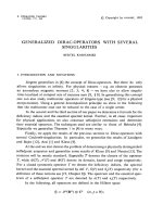
Figure 3: A graph G corresponding to the sequence = (+1, −1, +1, +1, −1, −1, +1, −1).
The dashed lines represent the pairing σ = {1, 6}, {2, 3}, {4, 5}, {7, 8}} .

1.3

Quotient graphs and quotient trees

We recall now the construction of Dykema and Haagerup [DH04a]. For integer k ≥ 1 let
G be an oriented k–gon graph with consecutive vertices v1 , . . . , vk and edges e1 , . . . , ek
(edge ei connects vertices vi and vi+1 ). The vertex v1 is distinguished, see Figure 3. We
encode the information about the orientations of the edges in a sequence (1), . . . , (k)
where (i) = +1 if the arrow points from vi+1 to vi and (i) = −1 if the arrow points from
vi to vi+1 . The graph G is uniquely determined by the sequence and sometimes we will
explicitly state this dependence by using the notation G .
Let σ = {i1 , j1 }, . . . , {ik/2 , jk/2 } be a pairing of the set {1, . . . , k}, i.e. pairs {im , jm }
are disjoint and their union is equal to {1, . . . , k}. We say that σ is compatible with if
(i) + (j) = 0

for every {i, j} ∈ σ.

(4)

It is a good idea to think that σ is a pairing between the edges of G, see Figure 3. For
each {i, j} ∈ σ we identify (or, in other words, we glue together) the edges ei and ej in
such a way that the vertex vi is identified with vj+1 and vertex vi+1 is identified with vj
and we denote by Tσ the resulting quotient graph. Since each edge of Tσ origins from a
pair of edges of G, we draw all edges of Tσ as double lines. The condition (4) implies that
each edge of Tσ carries a natural orientation, inherited from each of the two edges of G it
comes from, see Figure 4.
From the following on, we consider only the case when the quotient graph Tσ is a
tree. One can show [DH04a] that the latter holds if and only if the pairing σ is non–
crossing [Kre72]; in other words it is not possible that for some p < q < r < s we have
{p, r}, {q, s} ∈ σ. The name of the non–crossing pairings comes from their property that

on their graphical depictions (such as Figure 3) the lines do not cross. Let the root R of
the tree Tσ be the vertex corresponding to the distinguished vertex v1 of the graph G.
the electronic journal of combinatorics 13 (2006), #R62

5


Figure 4: The quotient graph Tσ corresponding to the graph from Figure 3. The root R
of the tree Tσ is encircled.

1.4

How to generalize the Cauchy identity? (continued)

Let us come back to the discussion from Section 1.2. We consider the polygon G corresponding to
= ( +1 , −1 , +1 , −1 ).
l times l times l times l times

All possible non-crossing pairings σ which are compatible with are depicted on Figure 5
and it easy to see that the corresponding quotient tree Tσ has exactly the form depicted
on Figure 2.
In this way we managed to find relatively natural combinatorial objects, the number
of which is given by the right-hand side of the Cauchy identity (1). After some guesswork
we end up with the following conjecture (please note that the usual Cauchy identity (1)
corresponds to m = 2).
Theorem 2 (Generalized Cauchy identity). For integers l, m ≥ 1 there are exactly
mml pairs (σ, <), where σ is a non-crossing pairing compatible with
= ( +1 , −1 , +1 , −1 , . . .)

(5)

l times l times l times l times
2m blocks, i.e. total of 2ml elements

and < is a total order on the vertices of Tσ which is compatible with the orientations of
the edges.
Above we provided only vague heuristical arguments why the above conjecture could
be true. Surprisingly, as we shall see in the following, Theorem 2 is indeed true.
The formulation of Theorem 2 is combinatorial and therefore appears to be far from its
motivation, the usual Cauchy identity (1), which is formulated algebraically, nevertheless
for each fixed value of m one can enumerate all ‘classes’ of pairings compatible with (5)
the electronic journal of combinatorics 13 (2006), #R62

6


Figure 5: A graph T corresponding to sequence = ( +1 , −1 , +1 , −1 ). The dashed
l times l times l times l times

lines denote a pairing σ for which the quotient graph Tσ is depicted on Figure 2.
and for each class count the number of compatible orders <. To give to the Reader a
flavor of the algebraic implications of Theorem 2, we present the case of m = 3 [DY03]
33l =
p+q=l

3p
p, p, p

3q
+3

q, q, q

p+q+r=l−1
r +q =r+q+1
p +r =p+r+1

2p + p
p, p, p

2q + q
q, q, q

r+r +r
r, r , r

.

(6)

The complication of the formula grows very quickly and already for m = 4 the appropriate
´
expression has a length of a half page of a typed text [Sni03].

1.5

Historical overview: operator algebras, free probability and
triangular operator T

The history presented in Sections 1.2–1.4 of finding the generalization of the Cauchy
identity is too nice to be true and indeed it is not the way how Theorem 2 was postulated.

As we shall see in the following, the path towards this result led not through combinatorics
but through the theory of operator algebras. Since this section is very loosely connected
with the rest of this article, Readers not interested in theory operator algebras may skip
it without much harm.
1.5.1

Invariant subspace conjecture

One of the fundamental problems of the theory of operator algebras is the invariant
subspace conjecture which asks if for every bounded operator x acting on an infinitedimensional Hilbert space H there exists a closed subspace K ⊂ H such that K is nontrivial
the electronic journal of combinatorics 13 (2006), #R62

7


in the sense that K = {0}, K = H and which is an invariant subspace of x. Since for many
decades nobody was able to prove the invariant subspace conjecture in its full generality,
Dykema and Haagerup took the opposite strategy and tried to construct explicitly a
counterexample by the means of the Voiculescu’s free probability theory.
The free probability [VDN92, HP00] is a non-commutative probability theory with
the classical notion of independence replaced by the notion of freeness. Natural examples
which fit nicely into the framework of the free probability include large random matrices, free products of von Neumann algebras and asymptotics of large Young diagrams.
Families of operators which arise in the free probability are, informally speaking, very
non-commutative and for this reason they are perfect candidates for counterexamples to
the conjectures in the theory of operator algebras [Voi96].
The first candidate for a counterexample to the invariant subspace conjecture considered by Dykema and Haagerup was the circular operator, which unfortunately turned out
´
to have a large family of invariant subspaces [DH01, SS01]. Later on Haagerup [Haa01]
proved a version of a spectral theorem for certain non–normal operators and thus he constructed invariant subspaces for many classes of operators. This result gave very strong
restrictions on the form of a possible counterexample, namely the Brown spectral measure

[Bro86] of such an operator should be concentrated in only one point. It was a hint to
look for counterexamples among, so-called, quasinilpotent operators. In this way Dykema
and Haagerup [DH04a] initiated a study of the triangular operator T , which appeared at
that time to be a perfect candidate because it is quasinilpotent and it admits very nice
random matrix models.
1.5.2

Triangular operator T

The triangular operator T [DH04a] can be abstractly described as an element of a von
Neumann algebra A equipped with a finite normal faithful tracial state φ : A → C with
the non-commutative moments φ(T (1) · · · T (n) ) given by
φ(T

(1)

···T

(n)

1
(1)
(n)
E Tr(TN · · · TN )
N →∞ N

) = lim

(7)

for any n ∈ N and (1), . . . , (n) ∈ {−1, +1}, where we use the notation T +1 := T and
T −1 := T ; and where


t1,1 t1,2 · · · t1,n−1
t1,n
 0 t2,2 · · · t2,n−1
t2,n 


 .
. 
.
..
. 
.
TN =  .
.
. 
.
 .

tn−1,n−1 tn−1,n 
0
···
0
tn,n
is an upper-triangular random matrix, the entries (ti,j )1≤i≤j≤N of which are independent
1
centered Gaussian random variables with variance N .

Definition (7) is not very convenient and one can show [DH04a] that it is equivalent
to the following one: (n/2 + 1)! φ(T (1) · · · T (n) ) is equal to the number of pairs (σ, <)
the electronic journal of combinatorics 13 (2006), #R62

8


such that σ is a pairing compatible with and < is a total order on the vertices of Tσ
which is compatible with the orientation of the edges. The Reader may easily see that
the latter definition of T is very closely related to the results presented in this paper; in
particular Theorem 2 can be now equivalently stated as follows (in fact it is the form in
which Dykema and Haagerup stated originally their conjecture [DH04a]):
Theorem 3. If l, m ≥ 1 are integers then
φ

T l (T )l

m

=

mml
.
(ml + 1)!

Yet another approach to T is connected with the combinatorial approach to operatorvalued free probability [Spe98], namely T can be described as a certain generalized circular
element. Speaking very briefly, the non-commutative moments of T can be described as
´
certain iterated integrals [Sni03]. This approach turned out to be very fruitful: in this
´

way in our previous work [Sni03] we found the first proof of Theorem 2 and Theorem 3; a
different proof was later presented in [AH04]. Some other combinatorial results concerning
the non-commutative moments of T were obtained in [DY03].
Theorem 2 and Theorem 3 were conjectured by Dykema and Haagerup [DH04a] in the
hope that they might be useful in the study of spectral properties of T . Literally speaking, this hope turned out to be wrong since the later construction of the hyperinvariant
subspaces of T by Dykema and Haagerup [DH04b, Haa02] did not make use of Theorem
2 and Theorem 3, however it made use of one of the auxiliary results used in our proof
´
[Sni03] of these theorems. In this way, indirectly, Theorem 2 and Theorem 3 turned out
to be indeed helpful for their original purpose.
As we already mentioned, Dykema and Haagerup [DH04b, Haa02] constructed a family
of hyperinvariant subspaces of T and in this way the original motivation for studying the
operator T (as a possible counterexample for the invariant subspace conjecture) ended up
as a failure. There are still some investigations of the triangular operator T as a possible
counterexample for some other conjectures, for example [Aag04], however most of the
specialists do not expect any surprises in the theory of operator algebras coming from this
direction. In this article we would like to convince the Reader that the applications of
the triangular operator T in combinatorics and the classical probability theory constitute
a sufficient compensation for the lost hopes concerning its applications in the theory of
operator algebras.

1.6
1.6.1

Overview of this series of articles
Part I: Bijective proof of generalized Cauchy identities

In this article we shall prove the following result. Let l1 ≤ · · · ≤ lm be a weakly increasing
sequence of positive integers; we denote L = l1 + · · · + lm + 1. For 1 ≤ i ≤ m we set
i

=

+1 ,

−1 , . . . , (−1)i−1 , (−1)i , . . . ,

li times li−1 times

l1 times

the electronic journal of combinatorics 13 (2006), #R62

l1 times

+1 , −1

,

(8)

li−1 times li times

9


where

a
l times

denotes a, . . . , a. The Reader may restrict his/her attention to the most
l times

interesting case when l1 = l2 = · · · = l are all equal and
i

i

takes a simpler form

+1 , −1

=

.

l times l times
i times, i.e. a total of 2li elements

In this case m coincides with (5) and it is easy to show from the Raney lemma [Ran60]
´
that the set (β) below has mml elements [Sni03] hence Theorem 2 will follow from the
following stronger result.
Theorem 4 (The main result). Let m be as above. The algorithm MainBijection
described in this article provides a bijection between
(α) the set of pairs (σ, <), where σ is a pairing compatible with m and < is a total order
on the vertices of Tσ which is compatible with the orientations of the edges;
(β) the set of tuples (B1 , . . . , Bm ), where B1 , . . . , Bm are disjoint sets such that B1 ∪
· · · ∪ Bm = {1, . . . , L} and

|B1 | + · · · + |Bn | ≤ l1 + · · · + ln
holds true for each 1 ≤ n ≤ m − 1;
Alternatively, set (β) can be described as
(γ) the set of sequences (a1 , . . . , aL ) such that a1 , . . . , aL ∈ {1, . . . , m} and for each
1 ≤ n ≤ m − 1 at most l1 + · · · + ln elements of the sequence (ai ) belong to the set
{1, . . . , n};
where the bijection between sets (β) and (γ) is given by Bj = {k : ak = j}.
˜
Remark 5. The sequence (˜1 , . . . , aL ) can be regarded as a generalized parking function,
a
where ar = m + 1 − ar . Indeed, let (b1 , . . . , bL ) be its non-decreasing rearrangement; then
˜
the original sequence (a1 , . . . , aL ) contributes to (γ) iff b1 , . . . , bL are positive integers such
that b1+lm ≤ 1, b1+lm +lm−1 ≤ 2,. . . , b1+lm +···+l1 ≤ m which is a slighlty modified definition
of a parking function.
The bijection provided by the above theorem plays the central role in this series of
articles.
1.6.2

´
Part II: Combinatorial differential calculus [JS06a]

The bijections considered in Part I of this series (Section 3 and Section 4 of this article)
are far from being trivial and the Reader might wonder how did the author guess their
correct form and what is the conceptual idea behind them. To answer these questions we
´
would like to come back to our previous work [Sni03] where we provided the first proof
the electronic journal of combinatorics 13 (2006), #R62

10

of Theorem 2. The main idea was to associate a polynomial of a single variable to every
pair (σ, <) and by additivity to every graph G . The polynomials associated to as in
(5) with different values of m turned out to be related by a simple differential equation
and for this reason can be regarded as generalizations of Abel polynomials.
´
In Part II of this series [JS06a] (joint work with Artur Je˙ ) we present an analogue of
z
the differential calculus in which the role of polynomials is played by certain ordered sets
and trees. Our combinatorial calculus has all nice features of the usual calculus and has
an advantage that the elements of the considered ordered sets might carry some additional
´
information. In this way our analytic proof from [Sni03] can be directly reformulated in
our new language of the combinatorial calculus; furthermore the additional information
carried by the vertices determines uniquely the bijections presented in Part I of this series.
1.6.3

´
Part III: Multidimensional arc-sine laws [JS06b]

In Section 1.1.3 we presented how a bijective proof the usual Cauchy identity can be
used to extract some information about the behavior of the Brownian motion and in
particular to show the arc-sine law. It is therefore natural to ask if the bijective proof
of the generalized Cauchy identities presented in Part I could provide some information
about multidimensional Brownian motions.
In order to answer these questions we study in Part III of this series the asymptotic
behavior of the trees and bijections presented in Part I. Asymptotically, as their size
tend to infinity, these trees converge towards continuous objects such as multidimensional
Brownian motions and Brownian bridges. Our bijection behaves nicely in this asymptotic

setting and becomes a map between certain classes of functions valued in Rm−1 , which is
closely related to the Pitman transform and Littelmann paths. In this way we are able
to describe certain interesting properties of multidimensional Brownian motions and in
particular we prove a multidimensional analogue of the arc-sine law.

2
2.1

The main bijection
Structure of a planar tree. Order

¡

For a non–crossing pairing σ we can describe the process of creating the quotient graph
as follows: we think that the edges of the graph G are sticks of equal lengths with flexible
connections at the vertices. Graph G is lying on a flat surface in such a way that the
edges do not cross. For each pair {i, j} ∈ σ we glue together edges ei and ej by bending
the joints in such a way that the sticks should not cross. In this way Tσ has a structure
of a planar tree, i.e. for each vertex we can order the adjacent edges up to a cyclic shift
(just like points on a circle). We shall provide an alternative description of this planar
structure in the following.
Let us visit the vertices of G in the usual cyclic order v1 , v2 , . . . , vk , v1 by going along
the edges e1 , . . . , ek ; by passing to the quotient graph Tσ we obtain a journey on the graph
Tσ which starts and ends in the root R. The structure of the planar tree defined above
the electronic journal of combinatorics 13 (2006), #R62

11


Figure 6: Example of a tree such that the arrows on all the edges point towards the root.

Leafs l1 , l2 , . . . and bays b1 , b2 , . . . are marked.
can be described as follows: if we travel on the graphical representation of Tσ by touching
the edges by our left hand, we obtain the same journey. For each vertex of Tσ we mark
the time we visit it for the first time; comparison of these times gives us a total order ¡,
called preorder [Sta99], on the vertices of Tσ . For example, in the case of the tree from
Figure 4 we have v1 ¡ v2 ¡ v3 ¡ v5 ¡ v8 .

2.2

Pairing between leafs and bays

Suppose that U is an oriented planar tree with the property that the arrows on all the
edges are pointing towards the root R; in other words R x holds true for every vertex
x. We shall also assume that the tree U consists of at least two vertices.
We call a pair of edges {e, f } a bay if edges e, f share a common vertex v and are
adjacent edges (adjacent with respect to the structure of the planar tree) and arrows on
e and f point towards the common vertex v. It is convenient to represent a bay as the
corner between edges e and f , cf Figure 6.
A vertex is called a leaf if it is connected to exactly one edge and it is different from
the root R, cf Figure 6.
Let us travel on the tree U (we begin and end at the root R) in such a way that we
always touch the edges of the tree by our left hand. We say that a passage along an edge
is negative if the arrow on the edge coincides with the direction of travel; otherwise we
call it a positive passage (the origin of this convention is the following: if U = Tσ is a
quotient tree coming from a polygonal graph G , where = ( (1), . . . , (k)) then the sign
of the n-th step coincides with the sign of (n)). It is easy to see that a bay corresponds
to a pair of consecutive passages: a negative and a positive one; similarly entering and
leaving a leaf corresponds to a pair of consecutive passages: a positive and a negative
one. In other words, the bays and the leafs correspond to the changes in the sign of
the passage. Since our journey begins with a positive passage and ends with a negative

one, therefore leafs l1 , . . . , lp+1 and bays b1 , . . . , bp are visited in the intertwining order
l1 , b1 , l2 , b2 , . . . , lp , bp , lp+1 . The number of the leafs (with the last leaf lp+1 excluded) is
the electronic journal of combinatorics 13 (2006), #R62

12


equal to the number of the bays, we can therefore consider a pairing between them given
by li → bi for 1 ≤ i ≤ p. In other words, to a leaf l we assign the first bay which is visited
in our journey after leaving l.

2.3

Catalan sequences

We say that = (1), . . . , (k) is a Catalan sequence if (1), . . . , (k) ∈ {−1, +1},
(1) + · · · + (k) = 0 and all partial sums are non-negative: (1) + · · · + (l) ≥ 0 for all
1 ≤ l ≤ k.
If is a Catalan sequence then there is no vertex v ∈ Tσ such that v R.
Lemma 6. For a Catalan sequence there exists a unique compatible pairing σ with the
property that R v for every vertex v ∈ Tσ . We call it Catalan pairing.
Proof. In the sequence let us replace each element +1 by a left bracket “ ” and let us
replace each element −1 by a right bracket “ ”. We leave it as an exercise to the Reader
to check that the pairing σ between corresponding pairs of left and right brackets is the
unique pairing with the required property.

2.4

The main bijection

The main result of this section is the algorithm MainBijection(T ) (with the auxiliary
algorithm SmallBijection(T )) which provides the bijection announced in Theorem 4.
In the remaining part of the article we will show that this algorithm indeed provides the
desired bijection.
Remark 7. At the beginning of each iteration of the loop in MainBijection T is a quotient
tree Tσ for some pairing σ which is compatible with i . In order to check it (formally: by
induction) we observe that li edges from each side of the root in the polygonal graph G i
are among those which were unglued in line 7 of MainBijection. These are the edges
which we remove in 8 of MainBijection. Formally, it corresponds to removal of the first
li and the last li elements from the sequence i and it is easily checked that the result is
equal to (− i−1 ). The change of the orientations of the edges in line 9 means the change
of sign of the corresponding sequence , hence after the iteration of the main loop in
MainBijection T = Tσ is a quotient tree corresponding to i−1 .
Remark 8. The operation of reversing the order < in line 9 of MainBijection means that
we do not change the labels assigned to the tree T but we change (by reversing) the way
we compare them. It follows that for in line 3 and in the function SmallBijection(T )
we consider the set of labels (which is the set of integer numbers) with its usual order <
if m − i is even and with the reverse of its usual order if m − i is odd.
Remark 9. Tree T in the algorithms MainBijection and SmallBijection is always a
quotient tree Tσ for some pairing σ which is compatible with some sequence . Each edge
of this tree was created from a pair of the edges of the polygonal graph G ; therefore the
operation of ungluing in line 9 of SmallBijection should be understood as ungluing of
the electronic journal of combinatorics 13 (2006), #R62

13


Figure 7: Algorithm MainBijection(T ), line 5. Subtree U was marked in gray.

Figure 8: Algorithm MainBijection(T ), line 7.

these original edges. On a formal level ungluing corresponds to removal of some pairs from
the pairing σ; similarly regluing in line 10 of SmallBijection corresponds to a creation
of new pairs in σ. Similar remarks concern lines 7, 11 of MainBijection.
Remark 10. Lines 4–6 of SmallBijection compute the bay BA, CA corresponding in
the tree U to the leaf D.

3
3.1

Proof of the correctness of the small bijection
Statement of the result

Let Tσ be a quotient tree and let < be an order on its vertices. We may always label the
vertices of Tσ (for example, with integer numbers) in such a way that the order of the
vertices coincides with the order of the corresponding labels. In this way we can view
SmallBijection as a map which to a pair (Tσ , <) (or, more formally, (σ, <)) associates
another pair of this form.
Theorem 11. Let = (1), . . . , (k) be a Catalan sequence. The function
SmallBijection as described above provides a bijection between
(A) the set of pairs (σ, <), where σ is a pairing compatible with and < is a total order
on the vertices of Tσ compatible with the orientation of the edges;

the electronic journal of combinatorics 13 (2006), #R62

14


Function MainBijection(T )
input : l1 ≤ · · · ≤ lm positive integers, L = l1 + · · · + lm + 1
T is a quotient tree corresponding to the Catalan sequence m

equipped with a total order < which is compatible with the
orientations of edges
output: disjoint sets B1 , . . . , Bm such that B1 ∪ · · · ∪ Bm = {1, . . . , L} and
|B1 | + · · · + |Bn | ≤ l1 + · · · + ln
holds true for each 1 ≤ n ≤ m − 1
1
2
3
4
5

6
7

8
9

10
11
12

13
14

label all vertices of T with numbers 1, . . . , L in such a way that each label appears
exactly once and the order < of vertices coincides with the order of the labels;
for i=m downto 1 do
T ← SmallBijection(T );
U ← tree {x ∈ T : x R};
Bi ← (labels of the vertices of U) ∩ {1, . . . , L};

/* cf. figure 7
*/
remove the labels of the vertices of U;
unglue all edges of tree U;
/* cf. figure 8

*/

remove li edges at each side of the vertex R;
change the orientation of all edges and reverse the order <;
/* cf. figure 9

*/

create sufficiently many artifical labels (integer numbers all different from
1, . . . , L) which are smaller than any label on tree T ;
glue the remaining edges of tree U by the Catalan pairing given by Lemma 6;
label the unlabeled vertices with artificial labels in such a way that on tree U
the orders < and ¡ coincide;
/* cf. figure 10
*/
end
return B1 , . . . , Bm ;

the electronic journal of combinatorics 13 (2006), #R62

15


Function SmallBijection(T )

input : T is a quotient tree correspondig to some sequence . The vertices of T
are equipped with some labels in such a way that the order of labels is
compatible with the orientations of the edges.
output: Tree T which is a quotient tree corresponding to the same sequence .
The vertices of T are labeled; the set of labels of this output tree coincides
with the set of the vertices of the input tree. More detailed description of
the output will be given in Theorem 11.
1
2
3
4
5
6
7

8
9
10
11

12
13

while orders < and ¡ do not coincide on {x ∈ T : x R} do
D ←the minimal element (with respect to <) such that R
and ¡ do not coincide on {x ∈ T : R x and x ≤ D} ;
U ← tree {x ∈ T : R x and x ≤ D} ;
C ←the successor of D in U with respect to ¡;
A ←father of C;
B ←son of A in U which is to the left of C;

labels ←set of labels carried by the vertices A, B, C, D;
/* cf. figure 11 and figure 14
remove the labels from the vertices A, B, C, D;
unglue the edges BA and CA ;

D and orders <

/* cf.

*/
figure 12 */

reglue these edges in the other possible way;
to unlabeled vertices give labels from labels in such a way that for each pair of
newly labeled vertices x < y iff x ¡ y;
/* cf. figure 13 and figure 15
*/
end
return T ;

the electronic journal of combinatorics 13 (2006), #R62

16


Figure 9: Algorithm MainBijection(T ), line 9. This graph was obtained from Figure 8
by removal of the dashed edges and it can be regarded as a certain polygonal graph G
with a number of trees attached to it. The orientation of all edges was reversed.

Figure 10: Algorithm MainBijection(T ), line 12. The polygonal graph G from figure

9 was glued according to the Catalan pairing. Artificial labels 100–103 were created to
label new vertices. The order of the labels was reversed therefore 103 < 102 < 101 <
100 < 7 < 4 < 1.
(B) the set of pairs (σ, <), where σ is a pairing compatible with
on the vertices of Tσ with the following two properties:
• on the set {x ∈ Tσ : x

R} the orders < and

¡ coincide;

• for all pairs of vertices v, w ∈ Tσ such that R
v

and < is a total order

v and R

w we have

w =⇒ v < w.

The remaining part of this section is devoted to the proof of this theorem.

3.2

Intermediate triples

Our strategy is to describe precisely which pairs (σ, <) (or alternatively, trees T ) might
arise in the intermediate steps of algorithm SmallBijection.

Definition. We call (σ, <, S) an intermediate triple if σ is a pairing compatible with , <
is a total order on the vertices of Tσ and S is one of the vertices of Tσ with the following
properties:
1. R

S and R ≤ S, where R denotes the root;

2. on the set {x : R

x and x ≤ S} the orders < and

¡ coincide;

3. for all pairs of adjacent vertices v, w ∈ Tσ such that v
w and v > w we have
R v and R w and the set {x ∈ Tσ : R x and S < x < v} is empty.
the electronic journal of combinatorics 13 (2006), #R62

17


Figure 11: Algorithm SmallBijection(T ), case D = B. The order of the vertices is
given by R ≤ A < B < C < D. Note that only edges belonging to the subtree U are
displayed.

Figure 12: The tree from Figure 11 after ungluing the edges BA and CA.

3.3

Startpoints and endpoints

Lemma 12. Intermediate triples (σ, <, S) for which S = R are in a one-to-one correspondence with the pairs (σ, <) which contribute to the set (A) and thus to the possible
input data of algorithm SmallBijection.
Proof. Suppose that (σ, <) contributes to (A); we set S = R. In order to show property
(2) of intermediate triples it is enough to observe that if x fulfills R x then also R ≤ x,
therefore the set {x ∈ Tσ : R x and x ≤ R} consists of only one element R. The other
two properties of intermediate triples hold true trivially.
Suppose that (σ, <, R) is an intermediate triple and suppose that there exists a pair of
vertices v, w such that v w and v > w. With no loss of generality we may assume that
the vertices v and w are adjacent (if this is not the case we may find a pair of adjacent
vertices v , w such that v
w and v > w on the path from the vertex v to the vertex
w). In the case w ≤ R property (3) shows that R
w and property (2) shows that
since R ¡ w therefore R < w which contradicts w ≤ R. In the case w > R the set
{x ∈ Tσ : R x and R < x < v} contains w which contradicts property (3). In this way
we proved that the total order < is compatible with the orientations of the edges.

the electronic journal of combinatorics 13 (2006), #R62

18


Figure 13: The tree from Figure 11 after regluing the edges BA and CA in a different
way. Please notice the change of the labels of the vertices A, B, C, D.

Figure 14: Algorithm SmallBijection(T ), case D = B. The order of vertices is given
by R ≤ A < C < D.
Lemma 13. Intermediate triples (σ, <, S) for which S is the maximal element (with
respect to the order <) of the set {x ∈ Tσ : x R} are in a one-to-one correspondence

with the pairs (σ, <) which contribute to the set (B). For such values of T = Tσ algorithm
SmallBijection terminates.
Proof. Suppose that (σ, <) contributes to the set (B); we define S to be the maximal
element (with respect to <) of the set {x ∈ Tσ : x R}. In order to prove that (σ, <, S)
is an intermediate triple it is enough to show property (3) of intermediate triples. Suppose
that there exist adjacent vertices v, w, such that v w and v > w; we shall consider now
three cases. The first case, R v, w is not possible, since then v < w would contradict
v > w. The second case, R
v
w would imply v ¡ w and hence v < w again
contradicts v > w. Therefore, the only remaining possibility is R w and R v. It is
not possible that R = w since then v
R would contradict the assumption that is a
Catalan sequence. In this way we proved that R w, R v which finishes the proof.
Suppose that (σ, <, S) is as in the statement of the lemma. In order to prove that
(σ, <) contributes to (B) it is enough to prove that for all vertices v, w such that R v
and R w we have v w =⇒ v < w. If this is not the case then there exist vertices
the electronic journal of combinatorics 13 (2006), #R62

19


Figure 15: The tree from Figure 14 after regluing the edges DA and CA in a different
way. Please notice the change of the labels of the vertices A, C, D.
v, w such that R w and v w, v > w. With no loss of generality we may assume that
the vertices v, w are adjacent hence R w contradicts R w.

3.4

The forward transformation

In this section we shall describe a certain invertible operation on intermediate triples
which will turn out to be equivalent to the algorithm SmallBijection. After a sufficient
number of iterations every intermediate triple corresponding to some element of (A) gets
transformed into an intermediate triple corresponding to some element of (B). In this way
the operation described in this section (which coincides with SmallBijection) provides
a bijection from (A) to (B).
Let (σ, <, S) be an intermediate triple and let D be the smallest element (with respect
to the order <) in the set {x : x R and x > S}. If no such element D exists, this means
that the triple (σ, <, S) is as in Lemma 13 and hence can be identified with an element
of the set (B); in other words our algorithm finished its work.
If (σ, <, D) is an intermediate triple, then we iterate our procedure.
We consider now the opposite case when (σ, <, D) is not an intermediate triple. Then
S is the maximal element (with respect to <) such that R S and such that on the set
{x ∈ Tσ : R x and x ≤ S} the orders < and ¡ coincide. Also, D is as prescribed by
line 2 of SmallBijection.
Let us denote by (σ , <) the pairing and the order which correspond to the value of T
in line 11 of algorithm SmallBijection.
Lemma 14. The triple (σ , <, S) given by the above construction is an intermediate triple.
The above procedure will stop after a finite number of steps.
Proof. We shall consider only the case when B = D, since the other case is analogous.
Conditions (1) and (2) are very easy to verify. To check condition (3) we need to find
the electronic journal of combinatorics 13 (2006), #R62

20


adjacent pairs of vertices v, w on tree Tσ for which v
w and v > w. Since condition
(3) is fulfilled for the tree Tσ it is enough to restrict our attention to such pairs which are

new, i.e. which were not present on the tree Tσ . Figure 13 indicates one such pair (namely
v = D, w = B and it is easy to check that this pair causes no problems) there might
be however some other such pairs which were not shown on Figure 12 because v ∈ U or
/
w ∈ U. It is easy to check that such new pairs must fall into one of the following three
/
categories: C < v < D, w = C (causes no problems); or v = D, A < w < D (impossible,
since it would imply that in the tree Tσ the vertex A is adjacent to the vertex w such that
A < w < D but (σ, <, S) is an intermediate triple, contradiction); or B < v < C, w = B
(causes no problems).
Note that in each step of our operation the cardinality of {x ∈ Tσ : R x and S ≤ x}
decreases. This shows that our procedure will eventually stop.

3.5

The backward transformation

In this section we shall describe the inverse of the transformation from Section 3.4.
Let (σ, <, S) be an intermediate triple and let S be the biggest element (with respect
to the order <) of the set {x : x
R and x < S}. If no such element exists it means
that (σ, <, S) is as in Lemma 12 hence our algorithm finished its work. If (σ, <, S ) is an
intermediate triple, we can iterate our procedure.
We consider now the opposite case when (σ, <, S ) is not an intermediate triple. It is
possible only when condition (3) of an intermediate triple is not fulfilled, namely there is
a pair of adjacent vertices B, D such that B D and B < D and {x : R x and S <
x < D} is a non-empty set. There may be many pairs B, D with this property; let us
select the one for which D takes its maximal value (with respect to <). Since (σ, <, S) is
an intermediate triple therefore {x : R x and S < x < D} is empty. It follows that the
only element which could possibly belong to {x : R x and S < x < D} is equal to S

and therefore S < D. In particular,
{x : R

x and S < x < D} = ∅.

(9)

Let U denote the subtree of Tσ which consists of the vertices {D}∪{x : R x and x ≤
S}. Let us change for a moment the orientation of the edge DB, as shown on the righthand side of Figure 16 and the right-hand side of Figure 18. It is easy to see that after
this change the tree U has the form as considered in Section 2.2, i.e. the arrows on all
edges are pointing towards the root and it has at least two vertices.
Let us consider the case when a corner formed in the vertex B by some edge on the
left and the edge DB on the right is a bay (on the right-hand side of Figure 16 this corner
corresponds to the pair of edges uB, DB). In this case let C denote the leaf corresponding
to this bay, as described in Section 2.2. We unglue the edges BA and BD and we reglue
them in the other way, as we described in Section 3.4, and thus we obtain a tree Tσ
corresponding to some pairing σ . Figure 17 describes the way how the vertices of the
original tree Tσ are identified with the vertices of Tσ . We shall prove in the following that
(σ , <, S) is an intermediate triple.
the electronic journal of combinatorics 13 (2006), #R62

21


Figure 16: On the left: a tree for which (σ, <, S ) is not an intermediate triple. Only
vertices belonging to the tree U were shown. On the right: the same tree with the
opposite orientation of the edge DB. In this case the pair of edges uB, DB forms a bay.
The order of the vertices is given by R ≤ A < B < C ≤ S < D.

Figure 17: The tree from the left-hand side of Figure 16 after ungluing and regluing

differently edges BA and BD. Please note that the labels carried by the vertices A, B, C, D
have changed.
It remains to consider the case when there is no bay in the vertex B formed by some
edge on the left and the edge DB on the right, cf Figure 18. We again unglue and reglue
differently the edges BA and BD; the resulting tree is denoted by Tσ . The identification
of the vertices of Tσ and Tσ is presented on Figures 18 and 19; please note that only
vertices A, B, D are nontrivially identified.
Lemma 15. The triple (σ , <, S) given by the above construction is an intermediate triple.
The above procedure will stop after a finite number of steps.
Proof. In the following we consider only the case presented on Figure 16 since the other
one is analogous.
Conditions (1) and (2) are very easy to verify. Condition (3) holds true for tree Tσ
hence there are only two reasons why it could fail for the tree Tσ . Firstly, there might
be some pair of adjacent vertices v, w on the tree Tσ for which v w and v > w which
the electronic journal of combinatorics 13 (2006), #R62

22


Figure 18: On the left: a tree for which (σ, <, T ) is not an intermediate triple. Only
vertices belonging to the tree U were shown. On the right: the same tree with the
opposite orientation of the edge BD. In this case the pair of edges BA, DB does not
form a bay. Order of vertices is given by R ≤ A < B < D.

Figure 19: The tree from the left-hand side of Figure 18 after ungluing and regluing
differently the edges BA and BD. Please note that the labels carried by the vertices
A, B, D have changed.
is new, i.e. which is not present in the tree Tσ . There are three possible cases: v = D,
C < w < D (impossible, since (9) implies C < w ≤ S < D and w ∈ U which contradicts
that C is a leaf of the tree U); or A < v < D, w = A (causes no problems); or v = C,

B < w < C (causes no problems).
The second reason why condition (3) could fail is that for some pair of adjacent vertices
v, w ∈ {A, B, C, D} such that v w and v > w the set
/
{x : R

x and S < x < v}

(10)

might be non-empty. Since tree Tσ fulfils condition (3) therefore the only element which
could possibly belong to the set (10) is D. This, however, is not the case since D was
chosen to be the maximal element in the set of the possible values of v.
Note that in each step of our operation the cardinality of the set {x ∈ Tσ : R
x and S ≤ x} increases. This shows that our procedure will eventually stop.
the electronic journal of combinatorics 13 (2006), #R62

23


The proof of the following lemma is straightforward and we leave it to the Reader.
Lemma 16. The operation described in Section 3.4 and the operation described in Section
3.5 are inverses of each other.
Thus, the proof of Theorem 11 is finished.
We will find the following result useful in Section 4.
Lemma 17. Let (σ, <, S), (σ , <, S ) be intermediate triples such that (σ , <, S ) is obtained from (σ, <, S) by a number of forward transformations from Section 3.4. We denote
U = {v ∈ Tσ : R v and v ≤ S} and U = {v ∈ Tσ : R v and v ≤ S }.
Then U ⊆ U . Furthermore, every element of the difference U \ U is bigger (both with
respect to the order < and ¡) than every element of the set U.
Secondly,

{v ∈ Tσ : R v} ⊇ {v ∈ Tσ : R v}.
(11)
Inductive proof is straightforward. Please note that, contrary to the order <, the order
and the lemma holds true for both choices of ¡.

¡ is different on the trees Tσ and Tσ
4

Proof of the correctness of the main bijection

We will prove Theorem 4, namely that MainBijection indeed provides the desired bijection.

4.1

Intermediate points

Our strategy is to describe possible intermediate outcomes of the algorithm
MainBijection.
Definition. We call Tσ , (Bi+1 , . . . , Bm ) an intermediate point for i (0 ≤ i ≤ m) if
1. σ is a pairing compatible with

i,

as defined in (8);

2. Tσ is a quotient tree with some of the vertices labeled with different elements of
{1, . . . , L};
3. let V be the set of unlabeled vertices of Tσ ; if i = m then V = ∅, if i < m then V is
a tree such that R ∈ V , V ⊆ {x ∈ Tσ : x R}, furthermore for all pairs such that
x y and y ∈ V we also have x ∈ V ;

4. for all pairs of labeled vertices such that x

y their labels fulfill x < y;

5. sets Bi+1 , . . . , Bm and the set of labels are disjoint and their union is equal to
{1, . . . , L};
6. |Bn | + · · · + |Bm | ≥ ln + · · · + lm + 1 for all i + 1 ≤ n ≤ m.
the electronic journal of combinatorics 13 (2006), #R62

24


4.2

Startpoints and endpoints

Lemma 18. There is a bijection between the elements of the set (α) (thus input data of
algorithm MainBijection) and the intermediate points corresponding to i = m.
There is a bijection between the elements of the set (β) and the intermediate points
corresponding to i = 0 (for which algorithm MainBijection terminates).

4.3

The forward transformation

˜
Lemma 19. After each iteration of the loop in MainBijection tuple T , (Bi , . . . , Bm )
˜
forms an intermediate point, where T denotes the tree T with all artificial labels removed.
Futhermore, on the set of the vertices with artificial labels the order ¡ coincides with the

order of the labels <.
Proof. We are going to use backward induction with respect to i.
Firstly, observe that in line 3 of MainBijection the computation of SmallBijection
is performed on a tree T which is as prescribed in point (A) of Theorem 11 therefore
afterwards T is as presecribed in point (B) of Theorem 11.
Furthermore, Lemma 17 shows that in line 6 of MainBijection all artificial labels will
˜
be removed. Therefore all artificial labels in T (equivalently, unlabeled vertices T ) after
the iteration of the loop must have been created in line 12.
This shows points (3) and (4) in the definition of an intermediate point.

4.4

The backward transform

We shall prescribe now the inverse of the transform prescribed in Section 4.3 (i.e. a single
interation of the loop in MainBijection). Since we simply have to reverse all steps of the
forward transformation, our description will be quite brief and we shall concentrate only
on the most critical points.
As we pointed out in the proof of Lemma 19 all artificial labels in T (equivalently,
˜
unlabeled vertices T ) after the iteration of the loop must have been created in line 12; in
other words, tree U consists of vertices carrying artificial labels.
Therefore, in order to undo line 12 of MainBijection we simply remove all artificial
labels and in order to undo line 11 we unglue all edges with both unlabeled ends.
In order to undo line 9 we change the orientation of all edges and reverse the order
of <. In order to undo line 8 to both sides of the root we attach li new edges with
appropriate orientations.
In order to undo line 7 we glue the unpaired edges according to the Catalan pairing.
Let U denote the set of unlabeled vertices. In order to undo line 6 we create |U| − |Bi |

artificial labels (which are integer numbers different from 1, . . . , L) which are smaller than
any element of the set {1, . . . , L} and we label the elements of U with these artificial labels
and the labels from the set Bi in such a way that the order ¡ of the vertices of U coincides
with the order < on the labels.

the electronic journal of combinatorics 13 (2006), #R62

25