Báo cáo toán học: "The Zeta Function of a Hypergraph" potx
Bạn đang xem bản rút gọn của tài liệu. Xem và tải ngay bản đầy đủ của tài liệu tại đây (204.17 KB, 26 trang )
The Zeta Function of a Hypergraph
Christopher K. Storm
Mathematics Department,
Dartmouth College,
Submitted: Aug 30, 2006; Accepted: Sep 22, 2006; Published: Oct 5, 2006
Mathematics Subject Classification: 05C38
Abstract
We generalize the Ihara-Selberg zeta function to hypergraphs in a natural
way. Hashimoto’s factorization results for biregular bipartite graphs apply,
leading to exact factorizations. For (d, r)-regular hypergraphs, we show that a
modified Riemann hypothesis is true if and only if the hypergraph is Ramanu-
jan in the sense of Winnie Li and Patrick Sol´e. Finally, we give an example to
show how the generalized zeta function can be applied to graphs to distinguish
non-isomorphic graphs with the same Ihara-Selberg zeta function.
1. Introduction
The aim of this paper is to give a non-trivial generalization of the Ihara-Selberg zeta
function to hypergraphs and show how our generalization can be thought of as a zeta
function on a graph. We will be concerned with producing generalizations of many
of the results known for the Ihara-Selberg zeta function: factorizations, functional
equations in specific cases, and an interpretation of a “Riemann hypothesis.” We
will also look at some of the properties of hypergraphs that are determined by our
generalization.
Later in this section, we will give the appropriate hypergraph definitions and path
definitions necessary for the zeta function. Keqin Feng and Winnie Li give an Alon-
Boppana type result for the eigenvalues of the adjacency operator of hypergraphs [8]
the electronic journal of combinatorics 13 (2006), #R84 1
which will motivate a definition for Ramanujan hypergraphs given by Li and Sol´e [14].
We will also give the appropriate definitions to define a “prime cycle” in a hypergraph
and give a formal definition of the zeta function.
Section 2 is concerned with generalizing a construction of Motoko Kotani and
Toshikazu Sunada [12]. The prime cycles in the hypergraph will correspond exactly
to admissible cycles in a strongly connected, oriented graph. This will let us write
the zeta function as a determinant involving the Perron-Frobenius operator T of the
strongly connected, oriented graph. The zeta function will look like det(I − uT )
−1
,
which is a rational function of the form one divided by a polynomial.
In Section 3 we explore in more detail the connection between a hypergraph
and its associated bipartite graph and what happens as prime cycles are represented
in the bipartite graph. This will allow us to realize the zeta function in terms
of the Ihara-Selberg zeta function of the bipartite graph. Theorem 10 details this
connection in full. We remark that our generalization is non-trivial in the sense
that there are infinitely many hypergraphs whose generalized zeta function is never
the Ihara-Selberg zeta function of a graph. We then get very nice factorization
results from Ki-Ichiro Hashimoto’s work [11], found in Theorem 16. As corollaries
to Hashimoto’s factorization results, we will be able to give functional equations
and connect the Riemann hypothesis to the Ramanujan condition for a hypergraph.
Theorem 24 shows that a Riemann hypothesis is true if and only if the hypergraph
is Ramanujan. We will also show how our zeta function fits into hypergraph theory
and can give information about whether a hypergraph is unimodular and about some
coloring properties for the hypergraph. These results are not new but more a matter
of framing previously known work in this context.
Finally, in Section 4 we show how this generalization can actually be applied
to graphs. One impediment to the Ihara-Selberg zeta function being truly useful
as a graph invariant is that two k-regular graphs are cospectral—their adjacency
operators have the same spectrum—if and only if they have the same zeta function
[16, 20]. We will examine an example of two 3-regular graphs constructed by Harold
Stark and Audrey Terras [22] which have the same zeta function but can be shown
explicitly to be non-isomorphic by computing our zeta function in an appropriate
way.
For the rest of this section, we fix our terminology and definitions. For the most
part, we are following [8, 14] for our definitions. A hypergraph H = (V, E) is a set
of hypervertices V and a set of hyperedges E where each hyperedge is a nonempty
set whose elements come from V , and the union of all the hyperedges is V . We
note that a hypervertex may not be repeated in the same hyperedge; although, with
appropriate care it is easy to generalize to this case. We allow hyperedges to repeat.
the electronic journal of combinatorics 13 (2006), #R84 2
A hypervertex v is incident to a hyperedge e if v ∈ e. Finally, we call the cardinality
of a hyperedge e, denoted |e|, the order of the hyperedge.
Using the incidence relation, we can associate a bipartite graph B to H in the
following way: the vertices of B are indexed by V (H) and E(H). Vertices v ∈ V (H)
and e ∈ E(H) are adjacent in B if v is incident to e. Given a hypergraph H, we
will denote by B
H
the bipartite graph formed in this manner. Given a hypergraph
H, we can construct its dual H
∗
by letting its hypervertex set be indexed by E(H)
and its hyperedges by V (H). We can use the bipartite graph to then construct the
appropriate incidence relation.
The associated bipartite graph is a very important tool in the study of hyper-
graphs. For now, we can use it to define an adjacency matrix for H. The adjacency
matrix A is a matrix whose rows and columns are parameterized by V (H). The
ij-entry of A is the number of directed paths in B
H
from v
i
to v
j
of length 2 with no
backtracking.
The adjacency matrix is symmetric—given a path of length 2 from v
i
to v
j
,
we traverse it backwards to get a path from v
j
to v
i
—so it has real eigenvalues. We
denote these eigenvalues, referred to as a set as the spectrum of the adjacency matrix,
by λ
1
, ··· , λ
|V (H)|
. The spectrum of H is defined to be the spectrum of A and satisfies
∆ ≥ λ
1
≥ λ
2
≥ ··· ≥ λ
|V (H)|
≥ −∆
for some ∆ ∈ R.
Definition 1. A hypergraph H is (d, r)-regular if:
1. Every hypervertex is incident to d hyperedges, and
2. Every hyperedge contains r hypervertices.
For a (d, r)-regular hypergraph, we have λ
1
= d(r − 1), and the fundamental
question becomes how large can the other eigenvalues be? Feng and Li, generalizing
a technique of Alon Nilli [19], give the following Alon-Boppana type result to address
this question [8]:
Theorem 2 (Feng and Li). Let {H
m
} be a family of connected (d, r)-regular hy-
pergraphs with |V (H
m
)| → ∞ as m → ∞. Then
lim inf λ
2
(H
m
) ≥ r −2 + 2
√
q as m → ∞,
where q = (d − 1)(r − 1) = d(r − 1) − (r − 1).
the electronic journal of combinatorics 13 (2006), #R84 3
Theorem 2 is the key ingredient for defining Ramanujan hypergraphs; however,
we need to explore the connection between H, B
H
, and H
∗
a bit more before we give
the definition. When H is (d, r)-regular, we also have that H
∗
is (r, d)-regular. Then
we can relate the adjacency operators of H, B
H
, and H
∗
as follows:
A(B
H
) =
0 M
t
M 0
, (1)
A(B
H
)
2
=
M
t
M 0
0
t
MM
=
A(H) + dI
V
0
0 A(H
∗
) + rI
E
, (2)
where M = M(V, E) is the incidence matrix of H, and I
V
and I
E
are identity matrices
with rows and columns parameterized by V and E respectively. Eq. (1) follows from
the definitions of the associated bipartite graph B
H
and by ordering the vertices in
B
H
in the same way as the hypervertices and hyperedges of H. To see Eq. (2), we
first note that the (i, j)-entry of A(B
H
)
k
is the number of paths of length k from
v
i
to v
j
[25]. Hence, the (i, j)-entry of A(B
H
)
2
is the number of paths of length 2
from v
i
to v
j
without backtracking plus the number of paths of length 2 from v
i
to
v
j
with backtracking. The adjacency operators of H and H
∗
account for the paths
without backtracking. The only way to have a path of length 2 from v
i
to v
j
with
backtracking is for i and j to be equal. Then, the number of such paths is either d
or r, depending on if v
i
comes from a hypervertex or a hyperedge, respectively, in H.
This accounts for the identity terms in the expression.
We let P (x), P
∗
(x), and Q(x) denote the characteristic polynomials of A(H),
A(H
∗
), and A(B
H
)
2
respectively. Then by Eq. (2), the characteristic polynomials
are related by
Q(x) = P (x − d)P
∗
(x − r). (3)
Since the eigenvalues of A(B
H
)
2
are all non-negative, this relation forces the eigen-
values of H and H
∗
to be at least −d and −r respectively. We can also relate P (x)
and P
∗
(x) directly as shown in [6]:
x
|V |
P
∗
(x − r) = x
|E|
P (x −d). (4)
This gives a very explicit connection between the spectra of H and H
∗
. When
d and r are not equal, comparing the powers of x in both sides of Eq. (4) gives
the obvious eigenvalue −d of H with multiplicity |V (H)|−|E(H)| or −r of H
∗
with
multiplicity |E(H)| − |V (H)|, depending on whether d < r or r < d.
Taking into account potential obvious eigenvalues and Theorem 2, we define Ra-
manujan hypergraphs:
the electronic journal of combinatorics 13 (2006), #R84 4
Definition 3 (Li and Sol´e). Let H be a finite, connected (d, r)-regular hypergraph.
We say H is a Ramanujan hypergraph if
|λ − r + 2| ≤ 2
(d − 1)(r − 1), (5)
for all non-obvious eigenvalues λ ∈ Spec(H) such that λ = d(r − 1).
This will be the basics of what we need for general hypergraph definitions. We
refer the interested reader to [2, 3, 8, 14] for more information on hypergraphs and
their spectra. We also point out that there are other potential definitions for Ra-
manujan hypergraphs that depend on the operators one wishes to study [13]. For
some explicit constructions of Ramanujan hypergraphs of the type treated here, we
refer the reader to [15]. We now turn our attention to the definition of the generalized
Ihara-Selberg zeta function of a hypergraph. We recommend the series of articles by
Harold Stark and Audrey Terras to the reader interested in current theory on Ihara-
type zeta functions on graphs [21, 22, 23]. Recently, there have also been a number
of generalizations of the zeta functions to digraphs as well as buildings [17, 18, 7].
To define our zeta function, we need the appropriate concept of a “prime cycle.”
A closed path in H is a sequence c = (v
1
, e
1
, v
2
, e
2
, ··· , v
k
, e
k
, v
1
), of length k = |c|,
such that v
i
∈ e
i−1
, e
i
for i ∈ Z/kZ. Note that this implies that v
1
∈ e
k
so that this
path really is “closed.” We say c has hyperedge backtracking if there is a subsequence
of c of the form (e, v, e). If we have hyperedge backtracking, this means that we
use a hyperedge twice in a row. In general, when we exclude cycles with hyperedge
backtracking, it will be permissible to return directly to a hypervertex so long as a
different hyperedge is used. We give an example of hyperedge backtracking in Figure
1. We denote by c
m
the m-multiple of c formed by going around the closed path m
times. Then, c is tail-less if c
2
does not have hyperedge backtracking. If, in addition
to having no hyperedge backtracking and being tail-less, c is not the non-trivial m-
multiple of some other closed path b, we say that c is a primitive cycle. Finally,
we can impose an equivalence relation on primitive cycles via cyclic permutation of
the sequence that defines the cycles. We call a representative of [c] a prime cycle.
We note that direction of travel does matter, so given a triangle in a graph, it can
actually be viewed as two prime cycles.
We now define the generalized Ihara-Selberg zeta function of a hypergraph:
Definition 4. For u ∈ C with |u| sufficiently small, we define the generalized Ihara-
Selberg zeta function of a finite hypergraph H by
ζ
H
(u) =
p∈P
1 −u
|p|
−1
,
the electronic journal of combinatorics 13 (2006), #R84 5
•
•
•
e
Figure 1: Hyperedge backtracking in a 3-edge e.
where P is the set of prime cycles of H.
Remark 5. A graph X can be viewed as a hypergraph where every hyperedge has
order 2. In this case, the definitions we’ve given—and in particular the definition
for hyperedge backtracking—correspond exactly to those needed to define prime cycles
in graphs. The zeta function ζ
X
(u) is, then, exactly the Ihara-Selberg zeta function
Z
X
(u).
In the next section, we will focus on giving an initial factorization of ζ
H
(u), which
represents the zeta function as a determinant of explicit operators. In Section 3, we
show more explicit factorizations, using results of Hyman Bass [1] and Hashimoto
[11]. Finally, in Section 4, we give an interpretation of this zeta function as a graph
zeta function and show how it can distinguish non-isomorphic graphs that are cospec-
tral.
Acknowledgments
The author would like to thank Dorothy Wallace and Peter Winkler for several
valuable discussions and comments in preparing this manuscript.
2. The Oriented Line Graph Construction
The goal of this section is to generalize the construction of an “oriented line graph”
which Kotani and Sunada [12] use to begin factoring the Ihara-Selberg zeta func-
tion. The idea is to start with a hypergraph and construct a strongly connected,
oriented graph which has the same cycle structure. By changing the problem from
hypergraphs to strongly connected, oriented graphs we will actually make finding an
explicit expression for ζ
H
(u) much simpler.
We first define some terms for oriented graphs. For an oriented graph, an oriented
edge e = {x, y} is an ordered pair of vertices x, y ∈ V . We say that x is the origin
the electronic journal of combinatorics 13 (2006), #R84 6
of e, denoted by o(e), and y is the terminus of e, denoted by t(e). We also have the
inverse edge ¯e given by switching the origin and terminus. We say that an oriented,
finite graph X
o
= (V, E
o
) is strongly connected if, for any x, y ∈ V , there exists an
admissible path c with o(c) = x and t(c) = y. A path c = (e
1
, ··· , e
k
) is admissible
if e
i
∈ E
o
and o(e
i
) = t(e
i−1
) for all i. We say that o(c) = o(e
1
) and t(c) = t(e
k
).
Let H be a finite, connected hypergraph. We label the edges of H: E =
{e
1
, e
2
, ··· , e
m
} and fix m colors {c
1
, c
2
, ··· , c
m
}. We now construct an edge-colored
graph GH
c
as follows. The vertex set V (GH
c
) is the set of hypervertices V (H). For
each hyperedge e
j
∈ E(H), we construct a |e
j
|-clique in GH
c
on the hypervertices in
e
j
by adding an edge, joining v and w, for each pair of hypervertices v, w ∈ e
j
. We
then color this |e
j
|-clique c
j
. Thus if e
j
is a hyperedge of order i, we have
i
2
edges
in GH
c
, all colored c
j
.
Once we’ve constructed GH
c
, we arbitrarily orient all of the edges. We then
include the inverse edges as well, so we finish with a graph GH
o
c
which has twice as
many colored, oriented edges as GH
c
.
Finally, we construct the oriented line graph H
o
L
= (V
L
, E
o
L
) associated with our
choice of GH
o
c
by
V
L
= E(GH
o
c
),
E
o
L
= {(e
i
, e
j
) ∈ E(GH
o
c
) × E(GH
o
c
); c(e
i
) = c(e
j
), t(e
i
) = o(e
j
)},
where c(e
i
) is the colored assigned to the oriented edge e
i
∈ E(GH
o
c
). If our hyper-
graph H was a graph to begin with, for any oriented edge e ∈ E(GH
o
c
), the only
oriented edge with the same color is ¯e. Then, the oriented line graph construction
given here is exactly that given by Kotani and Sunada [12]. See Figure 2 for an
example of this construction.
Proposition 6. Suppose H is a finite, connected hypergraph where each hypervertex
is in at least two hyperedges and which has more than two prime cycles. Then, the
oriented line graph H
o
L
is finite and strongly connected.
Proof. The vertices of H
o
L
are of the form {v, w}
e
where e ∈ E(H) and v, w ∈ e. This
catalogues using the hyperedge e to go from v to w. To show that H
o
L
is strongly
connected, we must show that given two subsequences {v
1
, e
1
, v
2
} and {v
k
, e
k
, v
k+1
}
with e
1
, e
k
∈ E(H), v
1
, v
2
∈ e
1
, and v
k
, v
k+1
∈ e
k
, there exists a path c in H of the form
c = (v
1
, e
1
, v
2
, e
2
, ··· , e
k−1
, v
k
, e
k
, v
k+1
) such that c has no hyperedge backtracking.
Since c has no hyperedge backtracking, we can use this path to construct a path in
H
o
L
which starts at {v
1
, v
2
}
e
1
and finishes at {v
k
, v
k+1
}
e
k
.
Since H is connected and every hypervertex is in at least 2 hyperedges, there
exists a path with no hyperedge backtracking d which begins with (v
1
, e
1
, v
2
, ···)
the electronic journal of combinatorics 13 (2006), #R84 7
•
v
1
•
v
2
•
v
3
•
v
4
•
v
5
a
b
c
d
•
v
1
•
v
2
•
v
3
•
v
4
•
v
5
a
1
a
2
a
3
a
4
a
5
a
6
b
1
b
2
b
3
b
4
b
5
b
6
c
1
c
2
d
1
d
2
•
a
1
•
a
2
•
a
3
•
a
4
•
a
5
•
a
6
•
b
1
•
b
2
•
b
3
•
b
4
•
b
5
•
b
6
•
c
1
•
c
2
•
d
1
•
d
2
Figure 2: We begin with a hypergraph H, already colored, in the top left. Then
we construct one possible edge-colored oriented graph GH
o
c
. From this graph, we
construct the corresponding oriented line graph. We notice that there are no edges
that go from a
i
to a
j
; this is because they represent the red edges in GH
o
c
.
the electronic journal of combinatorics 13 (2006), #R84 8
and finishes at vertex v
k
. Now there are two cases. Either the path used e
k
in the
last step to get to v
k
or it did not. If the path did not use e
k
, we can use e
k
to go to
v
k+1
, and we are done. In the second case, we need the additional hypothesis that
there are more than two prime cycles. We can get the desired path by leaving v
k
via a hyperedge different than e
k
. Then there is some cycle (which may have a tail)
which returns to v
k
via the other hyperedge. Then we can go from v
k
to v
k+1
via
e
k
. This yields the desired path. In essence, we need more than two prime cycles to
allow ourselves to “turn around” if we get going in the wrong direction. Hence, H
o
L
is strongly connected.
That H
o
L
is finite is clear since H is finite.
For m ≥ 1 ∈ Z, we let N
m
be the number of admissible closed paths of length m
in H
o
L
. Then, we define the zeta function of H
o
L
by
Z
o
H
o
L
(u) = exp
∞
m=1
1
m
N
m
u
m
. (6)
The initial factorization for this zeta function is determined in terms of the
Perron-Frobenius operator T : C(V
L
) → C(V
L
) given by
(T f)(x) =
e∈E
0
(x)
f(t(e)),
where E
0
(x) = {e ∈ E
o
|o(e) = x} is the set of all oriented edges with x as their
origin vertex.
Kotani and Sunada [12] give the details to let us factor Z
o
H
o
L
(u) in terms of its
Perron-Frobenius operator:
Theorem 7 (Kotani and Sunada). Suppose H
o
L
is a finite, oriented graph which
is strongly connected and not just a circuit. Then
Z
o
H
o
L
(u) = exp
∞
m=1
1
m
N
m
u
m
= det(I − uT )
−1
,
where T is the Perron-Frobenius operator of H
o
L
.
Proof. We only sketch the details:
1. Convergence in a disk about the origin follows from the Perron-Frobenius the-
orem [9].
2. The factorization was essentially given by Bowen and Lanford [5].
the electronic journal of combinatorics 13 (2006), #R84 9
We denote by P
o
L
the set of admissible prime cycles; then, we have the following
Euler Product expansion
Z
o
H
o
L
(u) =
p∈P
o
L
(1 −u
|p|
)
−1
which is Theorem 2.3 in [12]. Viewing the zeta function in this manner, we need
only show a correspondence between the prime cycles of H and the admissible prime
cycles of H
o
L
:
Proposition 8. There is a one-to-one correspondence between prime cycles of length
l in H and admissible prime cycles of length l in H
o
L
. In particular, the zeta function
of H can be written as
ζ
H
(u) = det(I − uT )
−1
,
where T is the Perron-Frobenius operator of H
o
L
.
Proof. We show the stated cycle correspondence; then, the factorization will follow
from the Euler Product expansion of Z
o
H
o
L
(u) and Theorem 7.
To show the cycle correspondence, we will actually show that there is a corre-
spondence between paths in H with no hyperedge backtracking and admissible paths
in H
o
L
. The cycle correspondence will then follow since all the relations imposed on
paths are the same.
Suppose v and w are hypervertices contained in a hyperedge e. Then we de-
note by {v, w}
e
the oriented edge in GH
o
c
with origin v, terminus w, and color
given by the color chosen for e. We let c = (v
1
, e
1
, v
2
, e
2
, ··· , v
k
, e
k
, v
k+1
) be a
path in H with no hypervertex backtracking. This corresponds to the path c
o
=
({v
1
, v
2
}
e
1
, {v
2
, v
3
}
e
2
, ··· , {v
k
, v
k+1
}
e
k
) in GH
o
c
. Since there is no hyperedge back-
tracking, i.e. e
i
= e
i+1
at every step, we change colors as we follow each oriented edge.
Then the corresponding path ˜c = (({v
1
, v
2
}
e
1
, {v
2
, v
3
}
e
2
), ({v
2
, v
3
}
e
2
, {v
3
, v
4
}
e
3
), ··· ,
({v
k−1
, v
k
}
e
k−1
, {v
k
, v
k+1
}
e
k
)) in H
o
L
is admissible with length k.
Similarly, given an admissible path in H
o
L
, we can realize it as a path in GH
o
c
which changes colors at every step. That means the corresponding path in H changes
hyperedges at every step; i.e., that it does not have hyperedge backtracking. The
lengths, then, are the same.
In particular, this theorem means that the zeta function is a rational function and
provides a tool to make some initial calculations. To get more precise factorizations,
we shall look more closely at the relationship between a hypergraph and its associated
bipartite graph.
the electronic journal of combinatorics 13 (2006), #R84 10
•
v
1
•
v
2
•
v
3
•
v
4
e
1
e
2
e
3
e
4
•
v
1
•
v
2
•
v
3
•
v
4
•
e
1
•
e
2
•
e
3
•
e
4
incidence
relation
Figure 3: An example of a primitive cycle of length 3 in a hypergraph and a corre-
sponding primitive geodesic of length 6 in its associated bipartite graph.
3. Further Factorizations
In the last section, we were able to realize the generalized Ihara-Selberg zeta function
as a determinant of explicit operators. In this section, we will see that by shifting
our view to the associated bipartite graph of a hypergraph, we can do much better.
Once we’ve established the relation between cycles in hypergraphs and cycles in
bipartite graphs that we need, we will draw very heavily from Hashimoto’s work on
zeta functions of bipartite graphs [11]. To help keep clear what structure we are
referring to, we will continue to call cycles in a hypergraph cycles but will call cycles
in the associated bipartite graph geodesics.
To motivate the relation we are looking for, we look at a simple example. In
Figure 3, we look at the primitive cycle given by c = (v
1
, e
1
, v
2
, e
3
, v
4
, e
2
, v
1
). This
corresponds to a primitive geodesic ˜c = (v
1
, {v
1
, e
1
}, e
1
, {e
1
, v
2
}, ··· , {e
2
, v
1
}, v
1
) in
the associated bipartite graph. In fact, this sort of correspondence is true in general:
Proposition 9. Let H be a finite, connected hypergraph with associated bipartite
graph B
H
. Then there is a one-to-one correspondence between prime cycles of length
l in H and prime geodesics of length 2l in B
H
.
the electronic journal of combinatorics 13 (2006), #R84 11
Proof. We will begin with a representative of a prime cycle of length l in H. Let
c = (v
1
, e
1
, ··· , v
l
, e
l
, v
1
) be a primitive cycle in H. Then we claim that
˜c = (v
1
, {v
1
, e
1
}, e
1
, ··· , v
l
, {v
l
, e
l
}, e
l
, {e
l
, v
1
}, v
1
) is a primitive geodesic in B
H
. It is
clear that ˜c is both closed and primitive if c is, so we need only check to be sure ˜c
has no backtracking or tails.
Let’s look at what hyperedge backtracking in the hypergraph means. We say
that c has hyperedge backtracking if we use the same hyperedge twice in a row. If
we think about the bipartite graph side, this means we leave a vertex in the set from
E(H), go to a vertex in the set V (H) and then backtrack to the vertex in E(H). Still
on the bipartite side, the only other way to backtrack is to go from a vertex in V (H)
to a vertex in E(H) and directly back. Thus, we would have the following sequence
in the hypergraph: (v
i
, e
i
, v
i
). This type of sequence is expressly disallowed unless
v
i
is repeated more than once in e
i
. If this happens, there is a multiple edge in B
H
representing this, which means we can actually return to the first vertex without
backtracking. Putting all of this together, we see that not hyperedge backtracking
in H is equivalent to not backtracking on the corresponding path in B
H
. Once we
know that backtracking isn’t an issue, having no tails also follows immediately since
backtracking in ˜c
2
would correspond to hyperedge backtracking in c
2
. Thus, each
prime cycle of length l in H corresponds to a prime geodesic of length 2l in B
H
.
We now look at prime geodesics in B
H
and show that they correspond to prime
cycles in H. Without loss of generality, we can assume that the first entry in a
representative of a prime geodesic in B
H
is a vertex parameterized by the set V (H).
If it is not, we simply shift the cycle one slot in either direction, and we will have
an appropriate representative because the graph is bipartite. Suppose the represen-
tative looks like ˜c = (v
1
, {v
1
, e
1
}, e
1
, ··· , v
l
, {v
l
, e
l
}, e
l
, {e
l
, v
1
}, v
1
); then we have the
following primitive cycle in H: c = (v
1
, e
1
, ··· , v
l
, e
l
, v
1
). This is a primitive cycle by
the same reasons as above since ˜c is a primitive geodesic. Also, |˜c| = 2l = 2|c|, so
we see that given a prime geodesic in B
H
, it corresponds to a prime cycle of half the
length in H.
This correspondence means that we can relate the generalized Ihara-Selberg zeta
function of a hypergraph to the Ihara-Selberg zeta function of its associated bipartite
graph.
Theorem 10. Let H be a finite, connected hypergraph such that every hypervertex
is in at least two hyperedges. Then,
ζ
H
(u) = Z
B
H
(
√
u).
the electronic journal of combinatorics 13 (2006), #R84 12
Proof. Let P
H
be the set of prime cycles on H and P
B
H
the set of prime geodesics on
B
H
. Then we rely on the previous proposition to write:
ζ
H
(u) =
p∈P
H
1 −u
|p|
−1
=
p∈P
H
1 − u
2|p|
1
2
−1
=
∈P
B
H
1 − u
||
1
2
−1
= Z
B
(
√
u).
As an immediate consequence of this relation, we see that, for an arbitrary hyper-
graph H which satisfies the conditions of Theorem 10 we can relate its zeta function
to the zeta function of its dual hypergraph H
∗
.
Corollary 11. Suppose H satisfies the conditions of Theorem 10. Then,
ζ
H
(u) = ζ
H
∗
(u)
Proof. H and H
∗
have the same associated bipartite graph, by definition. Then we
apply Theorem 10.
In addition, we can rewrite Hyman Bass’s Theorem [1] on factoring the zeta
function of a graph to give us a form of ζ
H
(u) which is more amenable to computation.
We first state Bass’s Theorem:
Theorem 12 (Bass). Let X be a finite, connected graph with adjacency operator A
and operator Q defined by D − I where D is the diagonal operator with the degree
of vertex v
i
in the ith slot of the diagonal. Let I be the |V | × |V | identity operator.
Then,
Z
X
(u) = (1 − u
2
)
χ(X)
det(I − uA + u
2
Q)
−1
where χ = |V |−|E| is the Euler Number of the graph X.
Given a hypergraph H, we apply Theorem 12 to factor Z
H
(u), giving us a com-
putable factorization of ζ
H
(u):
Corollary 13. Let H be a finite, connected hypergraph such that every hypervertex
is in at least two hyperedges. Let A
B
H
be the adjacency operator on B
H
, and let Q
B
H
be the operator on B
H
defined by D − I where D is the diagonal operator with the
degree of vertex v
i
in the ith slot of the diagonal. Let I be the m×m identity operator
where m = |V (H)|+ |E(H)|. Then
ζ
H
(u) = Z
B
H
(
√
u) = (1 − u)
χ(B
H
)
det(I −
√
uA
B
H
+ uQ
B
H
)
−1
,
the electronic journal of combinatorics 13 (2006), #R84 13
where χ(B
H
) = |V (B
H
)| − |E(B
H
)|.
Remark 14. We make a few notes, highlighting how we can compute each of the
terms that show up in Corollary 13:
1. Despite the square root that appears in this factorization, ζ
H
(u) is a rational
function. We see this clearly in the previous section, but we can also recover it
quickly by recalling that a bipartite graph only has prime cycles of even length.
2. The adjacency operator of B
H
can be quickly constructed from the incidence
matrix of H as in Eq. (1).
3. Similarly, we can construct the operator Q
B
H
quickly by considering the degrees
of vertices in the associated bipartite graph. If x is a vertex which comes from
V (H), we have d(x) is the number of hyperedges of which x is a member,
counting possible multiplicity. If x comes from E(H), then d(x) is the order of
the associated hyperedge. From these two facts, we can easily reconstruct Q
B
H
.
4. We also see that |V (B
H
)| = |V (H)| + |E(H)|. In addition, |E(B
H
)| can be
directly computed in two different ways via
|E(B
H
)| =
e∈E(H)
|e| =
v∈V (H)
{e ∈ E(H); v ∈ e}.
Example 15. We compute the generalized Ihara-Selberg zeta function of the hyper-
graph in Figure 3 in two ways. By going through the oriented line graph, we have
ζ
H
(u)
−1
= det(I − uT ) = (1 − u)(1 + u + u
2
− 5u
3
− 5u
4
− 5u
5
+ 4u
6
+ 4u
7
+ 4u
8
).
We can also compute the zeta function of the associated bipartite graph by using
Bass’s Theorem to realize
Z
B
H
(u)
−1
= (1 − u
2
)(1 + u
2
+ u
4
− 5u
6
− 5u
8
− 5u
10
+ 4u
12
+ 4u
14
+ 4u
16
).
Then we can directly see the relation ζ
H
(u) = Z
B
H
(
√
u).
We emphasize that Corollary 13 is mainly useful for computation. In general, the
diagonal entries of the Q matrix will not all be the same, making it quite difficult to
manipulate the factorization for theoretical results. Theorem 10 makes it clear that
the problem of factoring the generalized zeta function is really a problem of factoring
the zeta function of a bipartite graph. Fortunately, in [11], Hashimoto deals with
this question in great detail.
the electronic journal of combinatorics 13 (2006), #R84 14
We reformulate Hashimoto’s Main Theorem(III) [11] into our context to get the
following theorem:
Theorem 16. Suppose that H is a finite, connected (d, r)-regular hypergraph with
d ≥ r. Let n
1
= |V (H)|, n
2
= |E(H)|, and q = (d −1)(r −1). Let A be the adjacency
operator of H, and let A
∗
be the adjacency operator of H
∗
. Then one has
ζ
H
(u)
−1
= (1 − u)
−χ(B
H
)
(1 + (r − 1)u)
(n
2
−n
1
)
× det[I
n
1
− (A −r + 2)u + qu
2
]
= (1 − u)
−χ(B
H
)
(1 + (d −1)u)
(n
1
−n
2
)
× det[I
n
2
− (A
∗
− d + 2)u + qu
2
],
where −χ(B
H
) = n
1
(d −1) −n
2
= n
2
(r − 1) − n
1
.
Theorem 16 will provide the tool we need to produce theoretical results about the
generalized Ihara-Selberg zeta function on (d, r)-regular hypergraphs. The condition
that d ≥ r is actually not a problem. If H is a (d, r)-regular hypergraph; then, H
∗
is
(r, d)-regular. Thus, if d < r, we simply consider H
∗
as our starting point instead.
3.1. Consequences of the Factorization
Our first observation is that the zeta function of a hypergraph is a non-trivial gener-
alization of the Ihara-Selberg zeta function. By this, we mean that we can produce
an infinite number of zeta functions which are not the zeta function of any graph. A
simple way to produce zeta functions which did not come from a graph is encoded
in the next proposition.
Proposition 17. Suppose X is a finite graph with no vertices of degree 1, and H is
a finite hypergraph with every hypervertex in at least 2 hyperedges. Then,
1. The degree of the polynomial Z
X
(u)
−1
is 2|E(X)|.
2. The degree of the polynomial ζ
H
(u)
−1
is
e∈E(H)
|e|.
Proof. 1. Let X be a finite graph with no vertices of degree 1. Then by Bass’s
Theorem [1],
Z
X
(u)
−1
= (1 − u
2
)
|E|−|V |
× det(I − uA + u
2
Q).
The degree of the determinant term is 2|V |, and the degree of the explicit
polynomial is 2|E(X)|−2|V (X)|. Hence, the degree of Z
X
(u)
−1
is 2|E(X)|−
2|V (X)|+ 2|V (X)| = 2|E(X)|.
the electronic journal of combinatorics 13 (2006), #R84 15
2. Let H be a finite hypergraph with associated bipartite graph B
H
. Then by
Theorem 10,
ζ
H
(u)
−1
= Z
B
H
(
√
u)
−1
.
From the previous part, we see that the degree of Z
B
H
(
√
u)
−1
is |E(B
H
)|. We
can compute this explicitly as |E(B
H
)| =
e∈E(H)
|e|.
If a graph X has a vertex of degree 1, we can remove that vertex and the edge
to which it is adjacent without changing the zeta function. By removing all of these
types of vertices until we are left with a graph with every vertex having degree at least
2, we see that the zeta function of the graph we started with will be the zeta function
of a graph that satisfies Proposition 17. Hence, the inverse of the zeta function of
a graph will always have even degree. If we wish to exhibit hypergraphs with zeta
functions that did not arise from some graph, we need only find a hypergraph for
which
e∈E(H)
|e| is odd.
Example 18. In Example 15, we computed the zeta function of the hypergraph ap-
pearing in Figure 3. We see that the inverse of the zeta function has odd degree, so
this is an example of a hypergraph which produces a zeta function that no graph could
produce.
Before we turn to a discussion of the poles of the zeta function of a (d, r)-regular
hypergraph, we look at some of the symmetry that Hashimoto’s factorization gives
us. These functional equations are in the spirit of those given by Stark and Terras
in [21].
Corollary 19. Suppose that H is a finite connected (d, r)-regular hypergraph with
d ≥ r. Let n
1
= |V (H)|, n
2
= |E(H)|, q = (d − 1)(r − 1), and χ = χ(B
H
). Let A
be the adjacency operator of H, and let A
∗
be the adjacency operator of H
∗
. Finally,
suppose p(u) is a polynomial in u that satisfies p(u)
η
= ±(qu
2
)
η
p(
1
qu
)
η
. Then we
have the following functional equations for ζ
H
(u):
1. Λ
H
(u) = p(u)
n
1
(1 −u)
−χ
(1 + (r − 1)u)
n
2
−n
1
ζ
H
(u) = ±Λ
H
(
1
qu
).
2.
˜
Λ
H
(u) = p(u)
n
2
(1 −u)
−χ
(1 + (d − 1)u)
n
1
−n
2
ζ
H
(u) = ±
˜
Λ
H
(
1
qu
).
Proof. The strategy is really one of brute force factorization, using Theorem 16. By
Theorem 16, we can write ζ
H
(u) as
ζ
H
(u) = (1 − u)
χ
(1 + (r − 1)u)
(n
1
−n
2
)
× det[I
n
1
− (A − r + 2)u + qu
2
]
−1
.
the electronic journal of combinatorics 13 (2006), #R84 16
Substituting this expression into Λ
H
(u), we have
Λ
H
(u) = p(u)
n
1
× det[I
n
1
− (A −r + 2)u + qu
2
]
−1
.
We now algebraically manipulate the determinant term:
det[I
n
1
− (A − r + 2)u + qu
2
]
−1
= det[
qu
2
qu
2
− (A −r + 2)
qu
2
qu
+
qu
2
1
]
−1
=
1
qu
2
n
1
× det[
1
qu
2
− (A − r + 2)
1
qu
+
1
1
]
−1
=
1
qu
2
n
1
× det[
1
1
I
n
1
− (A −r + 2)
1
qu
+
q
(qu)
2
]
−1
.
We substitute this back into the expression for Λ
H
(u) and then use the given condition
for p(u)
n
1
:
Λ
H
(u) = p(u)
n
1
×
1
qu
2
n
1
× det[
1
1
I
n
1
− (A −r + 2)
1
qu
+
q
(qu)
2
]
−1
= ±(qu
2
)
n
1
p(
1
qu
)
n
1
×
1
qu
2
n
1
× det[
1
1
I
n
1
− (A − r + 2)
1
qu
+
q
(qu)
2
]
−1
= ±p(
1
qu
)
n
1
× det[
1
1
I
n
1
− (A − r + 2)
1
qu
+
q
(qu)
2
]
−1
= ±Λ
H
(
1
qu
).
This completes the first functional equation. The second one is identical, using
Hashimoto’s second factorization. We leave it as an exercise to the reader.
Remark 20. Using Corollary 19, we can write down several explicit functional equa-
tions for (d, r)-hypergraphs with d ≥ r.
1. Λ
H
(u) = (1 − u)
n
1
−χ
(1 + (r − 1)u)
(n
2
−n
1
)
(1 − qu)
n
1
ζ
H
(u) = Λ
H
(
1
qu
).
2.
˜
Λ
H
(u) = (1 − u)
n
2
−χ
(1 + (d −1)u)
(n
1
−n
2
)
(1 − qu)
n
2
ζ
H
(u) =
˜
Λ
H
(
1
qu
).
3. Ξ
H
(u) = (1 − u)
−χ
(1 + (r − 1)u)
(n
2
−n
1
)
(1 + qu
2
)
n
1
ζ
H
(u) = Ξ
H
(
1
qu
).
4.
˜
Ξ
H
(u) = (1 − u)
−χ
(1 + (d −1)u)
(n
1
−n
2
)
(1 + qu
2
)
n
2
ζ
H
(u) =
˜
Ξ
H
(
1
qu
).
the electronic journal of combinatorics 13 (2006), #R84 17
Now that we have several established functional equations, we turn to the next
important question for a zeta function. We will look at the location of the poles and
show that they very explicitly detect the Ramanujan condition on a (d, r)-regular
hypergraph.
We assume throughout that H is a (d, r)-regular hypergraph with d ≥ r. We let
n
2
= |E(H)|, n
1
= |V (H)|, q = (d−1)(r −1), and A be the adjacency operator on H.
Then, we have that n
2
≥ n
1
since d ≥ r. By Eq. (4), H has no obvious eigenvalues
−d. This will simplify our consideration of the Ramanujan condition on H.
We now want to focus on the determinant term in Hashimoto’s factorization.
Since A is symmetric, it is diagonalizable, so suppose Q diagonalizes A. Then,
det[I
n
1
− (A −r + 2)u + qu
2
] = det
Q[I
n
1
− (A − (r − 2)I
n
1
)u + qu
2
I
n
1
]Q
−1
= det[QI
n
1
Q
−1
− (QAQ
−1
− (r − 2)QI
n
1
Q
−1
)u + qu
2
QI
n
1
Q
−1
]
= det[I
n
1
− (QAQ
−1
− r + 2)u + qu
2
]
=
λ∈Spec(H)
[1 −(λ −r + 2)u + qu
2
].
This is the factorization we need to fully examine the relation between poles of
ζ
H
(u) and eigenvalues of H. The next two propositions detail the connection fully.
Proposition 21. Suppose H is a (d, r)-regular hypergraph with d ≥ r. Then,
1. ζ
H
(u) has a pole at u = 1 with multiplicity n
1
(d − 1) − n
2
= n
2
(r − 2) − n
1
=
−χ(B
H
).
2. ζ
H
(u) has a pole at u = −
1
r−1
with multiplicity n
2
− n
1
.
Proof. The first set of poles is contributed by the factor (1−u)
χ(B
H
)
given in Theorem
16. The second set is from the factor (1 + (r − 1)u)
(n
1
−n
2
)
.
Proposition 22. Suppose H is a (d, r)-regular hypergraph with d ≥ r. Let q =
(d −1)(r −1), then H is a Ramanujan hypergraph if and only if the poles of det[I
n
1
−
(A − r + 2)u + qu
2
]
−1
are distributed as below:
1. There is a simple pole at u = 1 and at u =
1
q
.
2. All other poles lie on the circle in the complex plane given by |r| =
1
√
q
.
the electronic journal of combinatorics 13 (2006), #R84 18
Proof. Since H is a (d, r)-regular hypergraph, there is an eigenvalue λ = d(r − 1).
We first rewrite the polynomial for this eigenvalue as
f(u) = qu
2
− (λ −r + 2)u + 1
= qu
2
− (q + 1)u + 1
= (1 − u)(1 −qu).
We can then see the roots at u = 1 and at u =
1
q
as claimed in part 1. We note that
if H is Ramanujan, the second eigenvalue is strictly smaller than d(r − 1), so these
poles are simple as claimed.
We now look at the eigenvalues which satisfy λ = d(r −1). Then the polynomial
f(u) = qu
2
− (λ −r + 2)u + 1 has roots at
u =
(r − 2 − λ) ±
(λ −r + 2)
2
− 4q
2q
.
Then u has Im(u) = 0 if and only if (λ − r + 2)
2
≤ 4q. This is true if and only if
|λ −r + 2| ≤ 2
√
q, which is true if and only if H is Ramanujan, by Definition 3 (there
are no obvious eigenvalues to consider by our assumption on d and r). In this case,
we can calculate the modulus of the roots by
|u|
2
=
(λ −r + 2)
2
4q
2
+
4q − (λ − r + 2)
2
4q
2
=
4q
4q
2
=
1
q
.
This gives us a complete characterization of the relation between the poles of
the generalized Ihara-Selberg zeta function and the Ramanujan condition on a hy-
pergraph. We can rewrite the previous two propositions into a modified Riemann
hypothesis.
Definition 23. Let H be a (d, r)-regular hypergraph with d ≥ r and q = (d−1)(r−1).
We then consider ζ
H
(q
−s
). We say that ζ
H
(q
−s
) satisfies the modified hypergraph
Riemann hypothesis if and only if for
Re s ∈ (0, 1),
(1 + (r − 1)q
−s
)
(n
2
−n
1
)
ζ
H
(q
−s
)
= 0 =⇒ Re s =
1
2
.
Then the previous two propositions can be summarized by
Theorem 24. For a (d, r)-regular hypergraph H, ζ
H
(q
−s
) satisfies the modified hy-
pergraph Riemann hypothesis if and only if H is a Ramanujan hypergraph.
the electronic journal of combinatorics 13 (2006), #R84 19
3.2. Some Hypergraph Properties
Before we move on and show how the zeta function can be interpreted as a graph
zeta function with a restricted cycle set, we show how some well-known hypergraph
properties fit into this framework. In particular, we will be interested in the case
when the zeta function is an even function. A graph is bipartite if and only if its
Ihara-Selberg zeta function is even, and we will see that the generalized zeta function
indicates some of the generalizations of “bipartite” to hypergraphs. The hypergraph
theorems we refer to are all from Chapter 20, Section 3 of Berge [2].
We let H = (V, E) be a finite hypergraph. An equitable q-colouring of H is a
partition (S
1
, ··· , S
q
) of the hypervertices into q classes such that for each i ∈ I and
for j, j
≤ q,
−1 ≤ |E
i
∩ S
j
| − |E
i
∩ S
j
| ≤ 1.
The smallest number q ≥ 2 for which there exists an equitable q-colouring is the
equitable chromatic number κ(H) of H. H is unimodular if for each S ⊂ V , the
subhypergraph H
S
admits an equitable bicolouring. A graph is unimodular if and
only if it is bipartite, so this definition is a generalization of bipartite for hypergraphs.
We now look at what it means for the generalized Ihara-Selberg zeta function to
be an even function:
Proposition 25. Let H be a hypergraph. Then, ζ
H
(u) = ζ
H
(−u) for all u ∈ C if and
only if every primitive cycle in H has even length.
Proof. We consider the power series expansion of the zeta function given in Definition
4. Then u appears to an odd power if and only if there is a prime cycle of odd length.
Hence, the zeta function must be even on a disk about the origin. Since it continues
to the inverse of a polynomial, it must be even throughout the complex plane.
This is all we need to reframe several of the results cited in [2]:
Theorem 26. Suppose H is a hypergraph with ζ
H
(u) an even function. Then, H is
unimodular.
Proof. This is Theorem 10 in Chapter 20 of [2].
Corollary 27. Suppose H is a hypergraph. Then ζ
H
(u) is even if and only if each
hypergraph H
, defined by taking hyperedges to be subsets of hyperedges of H and
hypervertex set to be the union of all the new hyperedges, satisfies κ(H
) ≤ 2.
We now return to the graph case and see how restricting the set of prime cycles
in a graph can give information which is more specific to the graph structure and
less dependent on the spectrum of the graph.
the electronic journal of combinatorics 13 (2006), #R84 20
• • • •
• • • •
• • • •
• • • •
Figure 4: Two cospectral graphs with different Ihara-Selberg zeta functions.
4. The Generalized Zeta Function as Applied to
Graphs
The ideas in this section are motivated, in part, by the question of determining if two
given graphs are isomorphic. We say two graphs are cospectral if the spectra of their
adjacency matrices are the same. For general graphs, the Ihara-Selberg zeta function
can be useful as a tool for distinguishing graphs since it’s possible to have cospectral
graphs with different zeta functions. Figure 4 gives an example of cospectral graphs
from [10] which have different zeta functions (there are also examples of graphs
which have the same Laplacian spectrum but different zeta functions). For k-regular
graphs, however, being cospectral is equivalent to having the same zeta function [16].
The problem is clearly illustrated by a result of Gregory Quenell [20]. We set up
some notation before we state his result.
The universal cover of a k-regular graph G is the infinite k-regular tree, which we
denote X
k
. We let Aut(X
k
) be the group of automorphisms of X
k
. Then the graph
G can be viewed as the quotient of X
k
by a subgroup H of Aut(X
k
) that acts freely.
We write G = H \X
k
; then the vertices of G are the orbits Hx of vertices in X
k
, and
Hx is adjacent to Hy if and only if each element of Hx is adjacent to some element
of Hy in X
k
. With this framework in mind, we state Quenell’s theorem:
Theorem 28 (Quenell). Let H \X
k
be an N-vertex, k-regular graph with no loops
or parallel edges. For each integer n ≥ 1, let
P
n
=
[h
i
]
H
⊂[t
n
]
Aut(X
k
)
L(C
H
(h
i
))
where [t
n
]
Aut(X
k
)
is the Aut(X
k
)-conjugacy class containing all length-n translations
in H and L(C
H
(h
i
)) denotes the length of a generator of the centralizer C
H
(h
i
) of h
i
in H.
Then the spectrum of H \ X
k
determines and is determined by the sequence
P
1
, P
2
, ··· , P
N
.
the electronic journal of combinatorics 13 (2006), #R84 21
•
••
•
••
r
r
r
Figure 5: A graph with a triangle singled out.
We interpret this theorem as saying that the spectrum of the adjacency operator
is determined and determines the number of primitive cycles of lengths 1, 2, ··· , N =
|V (X)|. These numbers figure prominently in the logarithmic derivative of Z
X
(u),
giving the zeta function connection. Hence, if we wish to try to use a zeta function to
distinguish cospectral regular graphs, we will need to restrict our paths in some way
to try to make them more accurately mimic the unique structure of a given graph.
We refer to Figure 5 to illustrate how the generalized Ihara-Selberg zeta function
might be used to do this. We will start with the set of all prime cycles in this graph.
Then we can throw out any prime cycle that uses two red edges in a row. We actually
will be throwing out infinitely many prime cycles when we do this. We could now
define a new zeta function using this smaller set of prime cycles in the same way as
before. It turns out that this is exactly the zeta function for the hypergraph formed
by replacing the red triangle with a 3-edge on the same vertices.
We could perform the same sort of construction for other graphs by replacing
cliques of any size with a hyperedge on the respective vertices. In this way, we would
hope that the path structure would more accurately mirror the structure of the graph
and not be as influenced by its spectrum. For the rest of this section we focus on an
example to illustrate this.
Figure 6 is an example of two graphs X
1
and X
2
which Stark and Terras con-
structed as a consequence of zeta function and covering considerations in [22]. These
graphs were constructed to have the same Ihara-Selberg zeta function and are thus
cospectral as well since they are 3-regular. It is fairly straight forward to check that
they are not isomorphic; however, we will use our zeta function to prove this, showing
how we can get more leverage by controlling paths more precisely.
Both X
1
and X
2
have exactly 4 triangles. We see this explicitly by considering
the coefficients of their characteristic polynomials as in [4] or by noting that the
coefficient of u
3
in Z
−1
X
1
(u) is −8, which is minus twice the number of triangles in X
1
[24]. We can find the triangles quickly by inspection. In X
1
, we’ve singled out two
disjoint triangles in red. In X
2
, all four triangles are represented in green.
the electronic journal of combinatorics 13 (2006), #R84 22
•
• •
•
• •
•
•
•
• •
•
•
• •
•
•
• •
•
•
• •
•
•
• •
•
X
1
r
r
r
r
r
r
•
• •
•
• •
•
•
•
• •
•
•
• •
•
•
• •
•
•
• •
•
•
• •
•
X
2
g
g
g
g
g
g
g
g
g
g
Figure 6: Two cospectral 3-regular graphs constructed by Stark and Terras in [22]
by zeta function and covering considerations.
the electronic journal of combinatorics 13 (2006), #R84 23
We now suppose that X
1
and X
2
are isomorphic. We change X
1
into a hypergraph
by replacing the red triangles with hyperedges on their vertices. We can now compute
the zeta function for this hypergraph. As before, we’ve restricted the prime cycles
on X
1
by throwing out any prime cycle that uses two red edges in a row.
If X
1
and X
2
are isomorphic, we should be able to repeat the transformation from
graph to hypergraph in X
2
and finish with isomorphic hypergraphs. There are four
possible ways to create a hypergraph from X
2
in the same manner as we did for X
1
.
For each green subgraph, we have a choice of two triangles to focus on, and there
are two such green subgraphs.
Now a simple comparison of generalized Ihara-Selberg zeta functions distinguishes
the graphs. All four of the hypergraphs constructed from X
2
actually have the same
zeta function. However, the hypergraph we constructed from X
1
has a different zeta
function. Hence, these two graphs are not isomorphic. Thus by making our paths
more specific to the structure of the graphs, we’ve actually managed to get around
Quenell’s result and give a zeta function proof that X
1
and X
2
are not isomorphic.
We should mention that there is a drawback to this method as well. We were
fortunate that our example had a relatively small number of triangles. As the num-
ber of non-disjoint triangles grows, we have to consider more and more potential
hypergraphs. Here, we only had to consider 4 potential hypergraphs constructed
from X
2
; however, this was a graph with quite a small number of triangles. Other
options would be to make every possible triangle into a hyperedge; then, you would
only have to compare one generalized Ihara-Selberg zeta function for each initial
graph. For this example, changing all four triangles into hyperedges and then com-
puting the generalized Ihara-Selberg zeta function of the resulting hypergraphs also
distinguishes the graphs. We hope to explore these methods more at a later date.
All computations of zeta functions referenced in this section are available from
the author by request.
References
[1] Hyman Bass. The Ihara-Selberg zeta function of a tree lattice. Internat. J.
Math., 3(6):717–797, 1992.
[2] Claude Berge. Graphs and Hypergraphs. North-Holland Publishing Co., 1973.
[3] Claude Berge. Hypergraphs. North-Holland Publishing Co., 1989.
[4] Norman Biggs. Algebraic graph theory. Cambridge University Press, 1974.
[5] R. Bowen and O. E. Lanford, III Zeta functions of restrictions of the shift
transformation. Proc. Symp. Pure Math., 14:43–50, 1970.
the electronic journal of combinatorics 13 (2006), #R84 24
[6] D. M. Cvetkovi´c, M. Doob, and H. Sachs. Spectra of graphs. Academic Press
[Harcourt Brace Jovanovich Publishers], 1980.
[7] Anton Deitmar and J. William Hoffman. The Ihara-Selberg zeta function for
PGL
3
and Hecke operators. Internat. J. Math., 17(2):143–155, 2006.
[8] Keqin Feng and Wen-Ch’ing Winnie Li. Spectra of hypergraphs and applica-
tions. Journal of Number Theory, 60(1):1–22, 1996.
[9] F. R. Gantmacher. The theory of matrices. Chelsea Publishing Co., 1959.
[10] Willem H. Haemers and Edward Spence. Enumeration of cospectral graphs.
European Journal of Combinatorics, 25(2):199–211, 2004.
[11] Ki-ichiro Hashimoto. Zeta functions of finite graphs and representations of p-
adic groups. Adv. Stud. Pure Math., 15:211 – 280, 1989.
[12] Motoko Kotani and Toshikazu Sunada. Zeta functions of finite graphs. J. Math.
Sci. Univ. Tokyo, 7:7–25, 2000.
[13] Wen-Ch’ing Winnie Li. Ramanujan hypergraphs. Geometric and Functional
Analysis, 14(2):380–399, 2004.
[14] Wen-Ch’ing Winnie Li and Patrick Sol´e. Spectra of regular graphs and hy-
pergraphs and orthogonal polynomials. European J. Combin., 17(5):461–477,
1996.
[15] Mar´ıa G. Mart´ınez, Harold M. Stark, and Audrey A. Terras. Some Ramanujan
hypergraphs associated to GL(n, F
q
). Proc. Amer. Math. Soc., 129(6):1623–
1629, 2001.
[16] Aubi Mellein. What does the zeta function of a graph determine? Louisiana
State University, Research Experience for Undergraduates program, 2001.
[17] Hirobumi Mizuno and Iwao Sato. Zeta functions of digraphs. Linear Algebra
Appl., 336:181–190, 2001.
[18] Hirobumi Mizuno and Iwao Sato. Zeta functions of oriented line graphs of graph
coverings. Discrete Math., 303(1-3):131–141, 2005.
[19] Alon Nilli. On the second eigenvalue of a graph. Discrete Math., 91(2):207–210,
1991.
[20] Gregory Quenell. Isospectrality conditions for regular graphs. Preprint, October
1998.
[21] Harold M. Stark and Audrey A. Terras. Zeta functions of finite graphs and
coverings. Adv. Math., 121(1):124–165, 1996.
[22] Harold M. Stark and Audrey A. Terras. Zeta functions of finite graphs and
coverings. II. Adv. Math., 154(1):132–195, 2000.
the electronic journal of combinatorics 13 (2006), #R84 25