Báo cáo toán học: "Hayman admissible functions in several variables" potx
Bạn đang xem bản rút gọn của tài liệu. Xem và tải ngay bản đầy đủ của tài liệu tại đây (281.34 KB, 29 trang )
Hayman admissible functions in several variables
Bernhard Gittenberger
∗
and Johannes Mandlburger
∗
Institute of Discrete Mathematics and Geometry
Technical University of Vienna
Wiedner Hauptstraße 8-10/104
A-1040 Wien, Austria
Submitted: Sep 12, 2006; Accepted: Nov 1, 2006; Published: Nov 17, 2006
Mathematics Subject Classifications: 05A16, 32A05
Abstract
An alternative generalisation of Hayman’s concept of admissible functions to
functions in several variables is developed and a multivariate asymptotic expansion
for the coefficients is proved. In contrast to existing generalisations of Hayman ad-
missibility, most of the closure properties which are satisfied by Hayman’s admissible
functions can be shown to hold for this class of functions as well.
1 Introduction
1.1 General Remarks and History
Hayman [20] defined a class of analytic functions
y
n
x
n
for which their coefficients y
n
can be computed asymptotically by applying the saddle point method in a rather uniform
fashion. Moreover those functions satisfy nice algebraic closure properties which makes
checking a function for admissibility amenable to a computer.
Many extensions of this concept can be found in the literature. E.g., Harris and
Schoenfeld [19] introduced an admissibility imposing much stronger technical requirements
on the functions. The consequence is that they obtain a full asymptotic expansion for
the coefficients and not only the main term. The disadvantage is the loss of the closure
properties. Moreover, it can be shown that if y(x) is H-admissible, then e
y(x)
is HS-
admissible (see [37]) and the error term is bounded. There are numerous applications of
H-admissible or HS-admissible functions in various fields, see for instance [1, 2, 3, 8, 9,
10, 11, 13, 20, 21, 22, 23, 24, 25, 26, 27, 28, 29, 30, 31, 32, 33, 34, 35, 36, 37, 38, 39].
∗
This research has been supported by the Austrian Science Foundation (FWF), grant P16053-N05 as
well as grant S9604 (part of the Austrian Research Network “Analytic Combinatorics and Probabilistic
Number Theory”).
the electronic journal of combinatorics 13 (2006), #R106 1
Roughly speaking, the coefficients of an H-admissible function satisfy a normal limit
law (cf. Theorem 1 in the next section). This has been generalised by Mutafchiev [30] to
different limit laws.
Other investigations of limit laws for coefficients of power series can be found in [4, 5,
16, 14, 15].
1.2 Generalisation to Functions in Several Variables
Of course, it is a natural problem to generalise Hayman’s concept to the multivariate case.
Two definitions have been presented by Bender and Richmond [6, 7] which we do not state
in this paper due to their complexity. The advantage of BR-admissibility and the even
more general BR-superadmissibility is a wide applicability. There is an impressive list
of examples in [7]. However, one loses some of the closure properties of the univariate
case. Moreover, the closure properties fulfilled by BR-admissible and BR-superadmissible
functions do not seem to be well suitable for an automatic treatment by a computer (in
contrary to Hayman’s closure properties, see e.g. [41] for H-admissibility or [12] for a
generalisation).
The intention of this paper is to define an alternative generalisation of Hayman’s
admissibility which preserves (most of) the closure properties of the univariate case. The
importance of the closure properties is that they enable us to construct new classes of
H-admissible functions by applying algebraic rules on a basic class of functions known
to be H-admissible. Conversely, it is possible to try to decompose a given function into
H-admissible atoms and use such a decomposition for an admissibility check which can
be done automatically by a computer. A first investigation in this direction was done
recently in [12] for bivariate functions whose coefficients are related to combinatorial
random variables. The univariate case was treated in [41].
In order to achieve our goal we will stay as close as possible to Hayman’s definition.
This allows us to prove multivariate generalisations of most of his technical auxiliary
results for the multivariate case. Then we can use essentially Hayman’s proof to show
the closure properties. We will require some technical side conditions which Hayman did
not need. However, verifying these needs asymptotic evaluation of functions which can
be done automatically using the tools developped by Salvy et al. (see [40, 42, 43]).
1.3 Comparison with BR-admissibility
Advantages
The advantage of H-admissibility is that the closure properties are more similar to those of
univariate H-admissibility which are more amenable to computer algebra systems. Indeed,
for H-admissible functions as well as a special class of multivariate function admissibility
check have successfully been implemented in Maple (see [12, 41] and remarks above).
the electronic journal of combinatorics 13 (2006), #R106 2
Drawbacks
H-admissibility seems to be a narrower concept than BR-admissibility. For an important
closure property, the product, we have to be more restrictive than Bender and Richmond
[7]. And the only (nonobvious) combinatorial example known not to be BR-admissible
which was presented by Bender and Richmond themselves is neither H-admissible.
Other remarks
If we consider functions in only one variable, then our concept of multivariate H-admissible
functions coincides with Hayman’s. This is not true for BR-admissible functions: Any
(univariate) H-admissible function is BR-admissible as well, but the converse is not true.
1.4 Plan of the paper
In the next section we recall Hayman’s admissibility. Then we present the definition
and some basic properties of H-admissible functions in several variables. Afterwards,
asymptotic properties for H-admissible functions and their derivatives are shown. In
Section 5, we characterise the polynomials P(z
1
, . . . , z
d
) in d variables with real coefficients
such that e
P
is an H-admissible function. This provides a basic class of H-admissible
functions as a starting point. The closure properties are shown in Section 6. The final
section lists some combinatorial applications.
2 Univariate Admissible Functions
Our starting point is Hayman’s [20] definition of functions whose coefficients can be com-
puted by application of the saddle point method in a rather uniform fashion.
Definition 1 A function
y(x) =
n≥0
y
n
x
n
(1)
is called admissible in the sense of Hayman (H-admissible) if it is analytic in |x| < R
where 0 < R ≤ ∞ and positive for R
0
< x < R with some R
0
< R and satisfies the
following conditions:
1. There exists a function δ(z) : (R
0
, R) → (0, π) such that for R
0
< r < R we have
y
re
iθ
∼ y(r) exp
iθa(r) −
θ
2
2
b(r)
, as r → R,
uniformly for |θ| ≤ δ(r), where
a(r) = r
y
(r)
y(r)
the electronic journal of combinatorics 13 (2006), #R106 3
and
b(r) = ra
(r) = r
y
(r)
y(r)
+ r
2
y
(r)
y(r)
− r
2
y
(r)
y(r)
2
.
2. For R
0
< r < R we have
y
re
iθ
= o
y(r)
b(r)
, as r → R,
uniformly for δ(r) ≤ |θ| ≤ π.
3. b(r) → ∞ as r → R.
For H-admissible functions Hayman [20] proved the following basic result:
Theorem 1 Let y(x) be a function defined in (1) which is H-admissible. Then as r → R
we have
y
n
=
y(r)
r
n
2πb(r)
exp
−
(a(r) − n)
2
2b(r)
+ o(1)
, as n → ∞,
uniformly in n.
Corollary 1 The function a(r) is positive and increasing for sufficiently large r, and
b(r) = o(a(r)
2
), as r → R.
If we choose r = ρ
n
to be the (uniquely determined) solution of a(ρ
n
) = n, then we
get a simpler estimate:
Corollary 2 Let y(x) be an H-admissible function. Then we have as n → ∞
y
n
∼
y(ρ
n
)
ρ
n
n
2πb(ρ
n
)
,
where ρ
n
is uniquely defined for sufficiently large n.
The proof of the theorem is an application of the saddle point method.
By means of several technical lemmas, which we do not state here, Hayman [20] proved
H-admissibility for some basic function classes. One of them is given in the following
theorem.
Theorem 2 Suppose that p(x) is a polynomial with real coefficients and that all but
finitely many coefficients in the power series expansion of e
p(x)
are positive, then e
p(x)
is H-admissible in the whole complex plane.
Furthermore he showed some simple closure properties which are satisfied by H-
admissible functions:
the electronic journal of combinatorics 13 (2006), #R106 4
Theorem 3 1. If y(x) is H-admissible, then e
y(x)
is H-admissible, too.
2. If y
1
(x), y
2
(x) are H-admissible, then so is y
1
(x)y
2
(x).
3. If y(x) is H-admissible in |x| < R and p(x) is a polynomial with real coefficients
and p(R) > 0 if R < ∞ and positive leading coefficient if R = ∞, then y(x)p(x) is
H-admissible in |x| < R.
4. Let y(x) be H-admissible in |x| < R and f(x) an analytic function in this region.
Assume that f(x) is real if x is real and that there exists a δ > 0 such that
max
|x|=r
|f(x)| = O
y(r)
1−δ
, as r → R.
Then y(x) + f(x) is H-admissible in |x| < R.
5. If y(x) is H-admissible in |x| < R and p(x) is a polynomial with real coefficients,
then y(x)+p(x) is H-admissible in |x| < R. If p(x) has a positive leading coefficient,
then p(y(x)) is also H-admissible.
3 Multivariate Admissible Functions: Definition and
Behaviour of Coefficients
In this section we will extend Hayman’s results to functions in several variables. In
particular, we will consider functions y(x
1
, . . . , x
d
) wich are entire in C
d
and admissible
in some range R ⊂ R
d
. R will be the domain of the absolute values of the function
argument, i.e., (|x
1
|, . . . , |x
d
|) ∈ R, whenever limits in C
d
are taken. We will for technical
simplicity assume that R is a simply connected set which contains the origin and has
(∞, . . . , ∞) as a boundary point.
3.1 Notations used throughout the paper
In the sequel we will use bold letters x = (x
1
, . . . , x
d
) to denote vector valued variables
(d-dimensional row vectors) and the notation x
n
= x
n
1
1
···x
n
d
d
. Moreover, inequalities
x < y between vectors are to be understood componentwise, i.e., x < y ⇐⇒ x
i
< y
i
for i = 1, . . . , d. r → ∞ means that all components of r tend to infinity in such a way
that r ∈ R. x
t
denotes the transpose of a vector or matrix x. Subscripts x
j
, etc. denote
partial derivatives w.r.t. x
j
, etc.
For a function y(x), x ∈ C
d
, a(x) = (a
j
(x))
j=1, ,d
denotes the vector of the logarithmic
(partial) derivatives of y(x), i.e.,
a
j
(x) =
x
j
y
x
j
(x)
y(x)
,
the electronic journal of combinatorics 13 (2006), #R106 5
and B(x) = (B
jk
(x))
j,k=1, ,d
denotes the matrix of the second logarithmic (partial) deriva-
tives of y(x), i.e.,
B
jk
(x) =
x
j
x
k
y
x
j
x
k
(x) + δ
jk
x
j
y
x
j
(x)
y(x)
−
x
j
x
k
y
x
j
(x)y
x
k
(x)
y(x)
2
,
where δ
jk
denotes Kronecker’s δ defined by
δ
jk
=
1 if j = k
0 if j = k
3.2 Definition and basic results
Like in the univariate case where we required asymptotic relations depending on whether
θ ∈ ∆(r) = (−δ(r), δ(r))
d
we will need a suitable domain ∆(r) for distinguishing the
behaviour of the function locally around the R (that means all arguments close to a real
number) from the behaviour far away from R. The geometry of multivariate functions is
Figure 1: Typical shape of |y(re
iϕ
, se
iθ
)|
much more complicated than that of univariate ones. For instance, for d = 2 dimensions
the typical shape of |y(re
iϕ
, se
iθ
)| for admissible functions is depicted in Figure 1. As
the figure shows, choosing straightforwardly ∆(r) = (−δ(r), δ(r))
d
will in general lead to
technical difficulties, for instance if max
θ∈∂∆(r)
y
re
iθ
has to be estimated. So in order
to avoid this, we have to adapt ∆(r) to the geometry of the function. This leads to the
following definition.
Definition 2 We will call a function
y(x) =
n
1
, ,n
d
≥0
y
n
1
···n
d
x
n
1
1
···x
n
d
d
(2)
with real coefficients y
n
1
···n
d
H-admissible in R if y(x) is entire and positive for x ∈ R
and x
j
≥ R
0
for all j = 1, . . . , d (for some fixed R
0
> 0) and has the following properties:
the electronic journal of combinatorics 13 (2006), #R106 6
(I) B(r) is positive definite and for an orthonormal basis v
1
(r), . . . , v
d
(r) of eigenvectors
of B(r), there exists a function δ : R
d
→ [−π, π]
d
such that
y
re
iθ
∼ y(r) exp
iθa(r)
t
−
θB(r)θ
t
2
, as r → ∞, (3)
uniformly for θ ∈ ∆(r) := {
d
j=1
µ
j
v
j
(r) such that |µ
j
| ≤ δ
j
(r), for j = 1, . . . , d}.
That means the asymptotic formula holds uniformly for θ inside a cuboid spanned
by the eigenvectors v
1
, . . . , v
d
of B, the size of which is determined by δ.
(II) The asymptotic relation
y
re
iθ
= o
y(r)
det B(r)
, as r → ∞, (4)
holds uniformly for θ /∈ ∆(r).
(III) The eigenvalues λ
1
(r), . . . , λ
d
(r) of B(r) satisfy
λ
i
(r) → ∞, as r → ∞, for all i = 1, . . . , d.
(IV) We have B
ii
(r) = o (a
i
(r)
2
), as r → ∞.
(V) For r sufficiently large and θ ∈ [−π, π]
d
\ {0} we have
|y(re
iθ
)| < y(r).
Remark 1 Condition (IV) of the definition is a multivariate analog of Corollary 1. We
want to mention that without requiring condition (IV), one can prove a weaker analog of
Corollary 1, namely B(r) = o(a (r)
2
) , as r → ∞, where · denotes the spectral
norm on the left-hand side and the Euclidean norm on the right-hand side. It turns out
that this condition is too weak for our purposes.
Remark 2 Note that for d = 1 (V) follows from the other conditions. We conjecture
that this is true for d > 1, too. However, we are only able to show that in the domains
θ = o
√
λ
min
/a(r)
2
and 1/θ = O
√
λ
min
the inequality (V) is certainly true
1
.
But since
√
λ
min
/a(r)
2
= o
1/
√
λ
min
there is a gap which we are not able to close.
Note that since B is a positive definite and symmetric matrix, there exists an orthog-
onal matrix A and a regular diagonal matrix D such that
B = A
t
DA. (5)
We will refer to these matrices several times throughout the paper.
1
λ
min
denotes the smallest eigenvalue of B(r)
the electronic journal of combinatorics 13 (2006), #R106 7
Lemma 1 Let y(x) be a function as defined in (2) which is H-admissible. Then, as
r → ∞, δ
j
(r)
2
λ
j
(r) → ∞ for j = 1, . . . , d.
Proof. If we take θ = δ
j
(r)v
j
(r) then we are at a point where (3) and (4) are both
valid. Taking absolute values in (3) we get
y
re
iθ
∼ y(r) exp
−
δ
j
(r)
2
λ
j
(r)
2
.
On the other hand (4) gives
y
re
iθ
= o
y(r)
det B(r)
.
Since det B(r) =
d
j=1
λ
j
(r) → ∞ we must have δ
j
(r)
2
λ
j
(r) → ∞.
Remark 3 The above lemma shows that δ cannot be too small. On the other hand, since
the third order terms in (I) vanish asymptotically, δ must tend to zero.
Theorem 4 Let y(x) be a function as defined in (2) which is H-admissible. Then as
r → ∞ we have
y
n
=
y(r)
r
n
(2π)
d/2
det B(r)
exp
−
1
2
(a(r) − n)B(r)
−1
(a(r) − n)
t
+ o(1)
, (6)
uniformly for all n ∈ Z
d
.
Proof. Let E =
j
µ
j
v
j
||µ
j
| ≤ δ
j
. Then we have y
n
r
n
= I
1
+ I
2
with
I
1
=
1
(2π)
d
···
E
y
re
iθ
e
inθ
t
dθ
1
··· dθ
d
and
I
2
=
1
(2π)
d
···
[−π,π]
d
\E
y
re
iθ
e
inθ
t
dθ
1
··· dθ
d
= o
y(r)
det B(r)
as can be easily seen from the definition of H-admissibility (cf. (4)).
By (3) and the substitution z = θ
(det B(r))/2 we have
I
1
∼
y(r)
(2π)
d
···
E
exp
i(a(r) − n)θ
t
−
1
2
θB(r)θ
t
dθ
1
··· dθ
d
=
y(r)
(π
2 · det B(r))
d
···
√
det B
2
·E
exp
icz
t
−
zB(r)z
t
det B(r)
dz
1
··· dz
d
,
the electronic journal of combinatorics 13 (2006), #R106 8
where c = (a −n)
2/ det B. Let A and D be the matrices of (5) Substituting z = wA
and extending the integration domain to infinity (which causes an exponentially small
error by Lemma 1) gives
I
1
∼
y(r)
(π
2 · det B(r))
d
∞
−∞
···
∞
−∞
exp
icA
t
w
t
−
1
det B(r)
d
j=1
λ
j
w
2
j
dw
1
··· dw
d
,
where λ
j
are of course the diagonal elements of D. Now observe that
∞
−∞
exp
−
λ
j
w
2
j
det B(r)
+ i(cA
t
)
j
w
j
dw
j
=
π det B(r)
λ
j
exp
(cA
t
)
2
j
det B(r)
4λ
j
and λ
1
···λ
d
= det B and thus
I
1
∼
y(r)
(2π)
d/2
det B(r)
exp
−
1
4
d
k=1
(det B(r)) · (cA
t
)
2
k
λ
k
.
With
(cA
t
)
2
k
=
2
det B(r)
d
j=1
(a
j
(r) − n
j
)A
kj
2
we get
d
k=1
(det B(r)) · (cA
t
)
2
k
4λ
k
=
d
k=1
1
2
√
λ
k
d
j=1
(a
j
(r) − n
j
)A
kj
2
=
(a(r) − n)A
t
D
−1
A(a(r) − n)
t
2
=
(a(r) − n)B(r)
−1
(a(r) − n)
t
2
as desired.
If we choose r = ρ
n
to be the solution of a(ρ
n
) = n, then we get a simpler estimate:
Corollary 3 Let y(x) be an H-admissible function. If n
1
, . . . , n
d
→ ∞ in such a way that
all components of the solution ρ
n
of a(ρ
n
) = n likewise tend to infinity, then we have
y
n
∼
y(ρ
n
)
ρ
n
n
(2π)
d
det B(ρ
n
)
,
where ρ
n
is uniquely defined for sufficiently large n, i.e., min
j
n
j
> N
0
for some N
0
> 0.
Remark 4 Note that in contrary to the univariate case, the equation a(ρ
n
) = n has not
necessarily a solution. There may occur dependencies between the variables which force all
coefficients to be zero if the index n lies outside a cone. Thus for those n the expression
on the right-hand side of (6) must, however, tend to zero and a(ρ
n
) = n cannot have a
solution.
Even if there is a solution, some components may remain bounded.
the electronic journal of combinatorics 13 (2006), #R106 9
4 Properties of H-admissible functions and their de-
rivatives
Lemma 2 H-admissible functions y(x) satisfy
a
re
h
∼ a(r), as r → ∞,
uniformly for |h
j
| = O (1/a
j
(r)).
Proof. Without loss of generality assume that d = 2. Since B is positive definite, we
have
B
11
B
22
− B
2
12
≥ 0 and thus |B
12
| ≤
B
11
B
22
= o(a
1
(r)a
2
(r))
by condition (IV) of the definition. Note that for positive definite matrices, every 2 × 2-
subdeterminant is nonnegative. Therefore considering only d = 2 is really no restriction.
Now define ϕ
1
(x
1
, x
2
) = a
1
(e
x
1
, e
x
2
) and ϕ
2
(x
1
, x
2
) = a
2
(e
x
1
, e
x
2
). Obviously
∂
∂x
1
ϕ
1
(x)
= B
11
(x) = o(a
1
(x)
2
) and
∂
∂x
2
ϕ
1
(x) = B
12
(x) = o(a
1
(x)a
2
(x)). Analogously, we have
∂
∂x
1
ϕ
2
(x) = o(a
1
(x)a
2
(x)) and
∂
∂x
1
ϕ
1
(x) = o(a
2
(x)
2
). Let |x
1
− x
1
| = O (1/a
1
(x
)) and
|x
2
− x
2
| = O (1/a
2
(x
)). Then
1
ϕ
2
(x
1
, x
2
)
−
1
ϕ
2
(x
1
, x
2
)
=
x
2
x
2
∂
∂x
2
ϕ
2
(x
1
, x)
ϕ
2
(x
1
, x)
2
dx
= o (x
2
− x
2
) = o
1
ϕ
2
(x
1
, x
2
)
, as x
1
, x
2
→ ∞,
which implies ϕ
2
(x
1
, x
2
) ∼ ϕ
2
(x
1
, x
2
) or, equivalently,
a
2
(x
1
, x
2
) ∼ a
2
(x
1
, x
2
) as x
1
, x
2
→ ∞. (7)
Now assume x
2
> x
2
and note that by Corollary 3 almost all coefficients y
n
of y(x)
for which min
j
n
j
is sufficiently large are nonnegative. Hence a
1
(x) and a
2
(x) must be
monotone in both variables for sufficiently large x
1
, x
2
. Therefore we get
1
ϕ
1
(x
)
−
1
ϕ
1
(x
)
=
x
2
x
2
∂
∂x
2
ϕ
1
(x
1
, x)
ϕ
1
(x
1
, x)
2
dx +
x
1
x
1
∂
∂x
1
ϕ
1
(x, x
2
)
ϕ
1
(x, x
2
)
2
dx
= o
a
2
(x
1
, x
2
)
a
1
(x
1
, x
2
)a
2
(x
1
, x
2
)
+ o (x
1
− x
1
)
Using (7) we finally obtain
1
ϕ
1
(x
)
−
1
ϕ
1
(x
)
= o
1
a
1
(x
1
, x
2
)
= o
1
ϕ
1
(x
)
which implies a
1
(x
) ∼ a
1
(x
). The asymptotic relation for a
2
is proved analogously and
completes the proof.
the electronic journal of combinatorics 13 (2006), #R106 10
Lemma 3 If y(x) is an H-admissible function then for n
j
> 0, j = 1, . . . , d, we have
y(r)
r
n
→ ∞ as r → ∞.
Moreover, for any given ε > 0 we have
a(r) = O (y(r)
ε
) and B(r) = O (y(r)
ε
)
as r → ∞.
Proof. The first relation is a trivial consequence of Theorem 4. So let us turn to the
other equations. Assume that there exists
¯
R such that for all r ≥
¯
R we have
a(r)
max
≥ y(r)
ε
.
This implies that for arbitrary h ∈ R
d
with only nonzero components, we have
j
a
j
(
¯
R + th) =
j
y
j
(
¯
R + th)
y(
¯
R + th)
(
¯
R
j
+ th
j
) ≥ y(
¯
R + th)
ε
· K
for t ≥ 0 and hence
j
y
j
(
¯
R + th)h
j
¯
R
j
h
j
+ t
y(
¯
R + th)
1+ε
≥ K.
Let k be such that
max
j
¯
R
j
+ th
j
h
j
=
¯
R
k
h
k
+ t.
Then
j
y
j
(
¯
R + th)h
j
y(
¯
R + th)
1+ε
≥
K
¯
R
k
h
k
+ t
.
Set g(t) = y(
¯
R + th). Therefore we have
g
(t)
g(t)
1+ε
≥
K
¯
R
k
h
k
+ t
and thus
ρ
0
g
(t)
g(t)
1+ε
dt ≥ K
log
¯
R
k
h
k
+ ρ
− log
¯
R
k
h
k
= K log
¯
R
k
+ ρh
k
¯
R
k
(8)
Now let ρ → ∞ and note that (8) is unbounded. On the other hand, the above integral
evaluates to
ρ
0
g
(t)
g(t)
1+ε
dt =
y(
¯
R)
−ε
− y(
¯
R + ρh)
−ε
ε
(9)
which is bounded for ρ → ∞ and we arrive at a contradiction.
the electronic journal of combinatorics 13 (2006), #R106 11
Corollary 4 For any ε > 0 we have, as r → ∞, det B(r) = O (y(r)
ε
).
Proof. Since B is the largest eigenvalue of B, we have det B ≤ B
d
. Hence the
assertion immediately follows from Lemma 3.
Lemma 4 Let k be fixed. Then an H-admissible function y(x) satisfies
y
r
1
+
kr
1
a
1
(r)
, . . . , r
d
+
kr
d
a
d
(r)
∼ e
kd
y(r
1
, . . . , r
d
)
for r
1
, . . . , r
d
→ ∞ (r → ∞)
Proof. For given h
1
, . . . , h
d
we have for some 0 < θ < 1
log y(r
1
+ h
1
, . . . , r
d
+ h
d
) − log y(r
1
, . . . , r
d
) =
d
j=1
y
z
j
(r
1
+ θh
1
, . . . , r
d
+ θh
d
)h
j
y(r
1
+ θh
1
, . . . , r
d
+ θh
d
)
=
d
j=1
h
j
r
j
+ θh
j
a
j
(r
1
+ θh
1
, . . . , r
d
+ θh
d
)
=
d
j=1
ka
j
(r
1
+ θh
1
, . . . , r
d
+ θh
d
)
1 + O
1
a
j
(r)
a
j
(r
1
+ θh
1
, . . . , r
d
+ θh
d
)
∼ kd
where we substituted h
j
= kr
j
/a
j
(r) and r
j
/(r
j
+θh
j
) = 1+O (1/a
j
(r)) in the penultimate
step and used Lemma 2 in the last step.
The next theorem shows that the coefficients of H-admissible functions satisfy a mul-
tivariate normal limit law.
Theorem 5 Let y(x) =
n≥0
y
n
x
n
be an H-admissible function. Moreover, let
˜
n = nA
t
,
where A is the orthogonal matrix defined in (5), and let
˜
a(r) = (˜a
1
(r), . . . , ˜a
d
(r)) = a ·A
t
be the vector of the logarithmic derivatives of y(x) w.r.t. the orthonormal eigenbasis of
B(r) given in the definition. Then we have, as r → ∞,
n s. t. ∀j: ˜n
j
≤˜a
j
(r)+ω
j
√
λ
j
(r)
y
n
r
n
∼
y(r)
(2π)
d/2
ω
d
−∞
···
ω
1
−∞
exp
−
1
2
d
j=1
t
2
j
dt
1
··· dt
d
Proof. Define N
j
= ˜a
j
(r), and
N
j
=
˜a
j
(r) + ω
j
2 det B(r)
, N
j
=
˜a
j
(r) + ω
j
2 det B(r)
the electronic journal of combinatorics 13 (2006), #R106 12
for some ω
j
< 0 < ω
j
. Let furthermore N
j
+ 2 ≤ n
j
≤ N
j
and D be the diagonal matrix
of (5). Then
n
1
+1
n
1
···
n
d
+1
n
d
exp
−
(x −
˜
a)D(r)
−1
(x −
˜
a)
t
2
dx
1
··· dx
d
≤ exp
−
(n −
˜
a)D(r)
−1
(n −
˜
a)
t
2
≤
n
n−1
exp
−
(x −
˜
a)D(r)
−1
(x −
˜
a)
t
2
dx
1
··· dx
d
This implies
N
1
+1
N
1
+2
···
N
d
+1
N
d
+2
exp
−
(x −
˜
a)D(r)
−1
(x −
˜
a)
t
2
dx
1
··· dx
d
≤
N
1
+1
n
1
=N
1
+2
···
N
d
+1
n
d
=N
d
+2
exp
−
(n −
˜
a)D(r)
−1
(n −
˜
a)
t
2
≤
N
1
N
1
+1
···
N
d
N
d
+1
exp
−
(x −
˜
a)D(r)
−1
(x −
˜
a)
t
2
dx
1
··· dx
d
By substituting x
j
= ˜a
j
(r) + t
j
λ
j
(r), dx =
det B(r) dt, the integral becomes
det B(r)
t
1
t
1
···
t
d
t
d
exp
−
1
2
d
j=1
t
2
j
dt
1
··· dt
d
with t
j
→ 0 and t
j
→ ω
j
.
Now set
˜
N :=
n ∈ N
d
such that for all j we have N
j
≤ ˜n
j
≤ N
j
. Then an applica-
tion of Theorem 4 gives
n∈
˜
N
y
n
r
n
∼
y(r)
(2π)
d/2
√
det B
n∈
˜
N
exp
−
(n − a)B
−1
(n − a)
t
2
=
y(r)
(2π)
d/2
√
det B
N
˜
n=N
exp
−
(
˜
n −
˜
a)D
−1
(
˜
n −
˜
a)
t
2
∼
1
(2π)
d/2
ω
1
ω
1
···
ω
d
ω
d
exp
−
1
2
d
j=1
t
2
j
dt
1
··· dt
d
the electronic journal of combinatorics 13 (2006), #R106 13
where in the last step the considerations above were applied. On the other hand the sum
∃j:n
j
<N
j
y
n
r
n
< εy(r) if all ω
j
are small enough.
Theorem 6 Let k ∈ R
d
be fixed. Then, as r → ∞,
∂
k
1
∂x
k
1
1
···
∂
k
d
∂x
k
d
d
y(r) ∼ y(r)
a
1
(r)
r
1
k
1
···
a
d
(r)
r
d
k
d
Proof. Set
¯
R
j
= r
j
1 +
1
a
j
(r)
. Then, if |z
j
| <
¯
R
j
for all j, we have by Lemma 4
|y(z)| =
n
y
n
z
n
≤
y
n
¯
R
n
= y(
¯
R) = O (y(r)) .
Let h =
¯
R − r =
r
1
a
1
(r)
, . . . ,
r
d
a
d
(r)
. Then we have
y(z) =
1
k
1
! ···k
d
!
∂
k
1
∂x
k
1
1
···
∂
k
d
∂x
k
d
d
y(r)(z − r)
k
and hence by Cauchy’s inequality we get
∂
k
1
∂x
k
1
1
···
∂
k
d
∂x
k
d
d
y(r)
≤
k
1
! ···k
d
!
h
k
1
1
···h
k
d
d
y(
¯
R)
O
y(r)
a
1
(r)
r
1
k
1
···
a
d
(r)
r
d
k
d
Now define (n)
k
:= n(n − 1) ···(n −k + 1) and observe that
r
k
1
1
···r
k
d
d
∂
k
1
∂x
k
1
1
···
∂
k
d
∂x
k
d
d
y(r) =
n
(n
1
)
k
1
···(n
d
)
k
d
y
n
r
n
=
1
+
2
with
1
=
n such that ∀j: |a
j
(r)−n
j
|≤ω
√
B
jj
(r)
(n
1
)
k
1
···(n
d
)
k
d
y
n
r
n
and
2
=
−
1
. In the range of summation we have (n
1
)
k
1
···(n
d
)
k
d
∼ a(r)
k
. Let
˜
n
as in Theorem 5 and set s
j
= n
j
− a
j
and ˜s
j
= ˜n
j
− ˜a
j
. Since A is orthogonal, we have
˜
s
2
= s
2
= ω
2
d
j=1
B
jj
the electronic journal of combinatorics 13 (2006), #R106 14
Hence the range of summation covers the set {n : ∀j : |˜a
j
(r)−˜n
j
| ≤ ω
λ
j
(r)}. Therefore
we obtain by means of Theorem 5
1
∼ C(ω)y(r)a(r)
k
with
1
π
d/2
ω
−ω
···
ω
−ω
exp
−
1
2
d
j=1
t
2
j
dt
1
··· dt
d
< C(ω) < 1.
On the other hand define
:=
n:∃j:|a
j
−n
j
|>ω
√
B
jj
(r)
.
Then we have
2
≤
(n
1
)
k
1
···(n
d
)
k
d
y
n
r
n
≤
n
k
y
n
r
n
≤
n
2k
y
n
r
n
1/2
y
n
r
n
1/2
= O
r
2k
∂
2k
1
∂x
2k
1
1
···
∂
2k
d
∂x
2k
d
d
y(r)
···
E
exp
−
1
2
d
j=1
t
2
j
dt
1
··· dt
d
1/2
,
with the integration domain E = (R
+
)
d
\ [0, ω]
d
. Therefore, since
r
2k
∂
2k
1
∂x
2k
1
1
···
∂
2k
d
∂x
2k
d
d
y(r) = O
y(r)a(r)
2k
,
we have for sufficiently large ω
1
+
2
−y(r)a(r)
k
< εy(r)a(r)
k
which completes the proof.
Lemma 5 Assume that there exist constants η > 0 and C > 0 such that for |z
j
−r
j
| < ηr
j
(j = 1, . . . , d) the matrix B satisfies |hB (z) h
t
| ≤ ChB(r)h
t
for all h ∈ R
d
. Furthermore,
assume regularity of y(z) in this region and that y(z) = 0. Then
log y
r
1
e
iθ
1
, . . . , r
d
e
iθ
d
= log y(r) + iθa(r)
t
−
1
2
θB(r)θ
t
+ ε(r, θ)
where
|ε(r, θ)| ≤
Cθ · θB(r)θ
t
η
. (10)
Proof. Set g(t) = log y
e
x
1
+ith
1
, . . . , e
x
d
+ith
d
for |t| ≤ η and some h with h = 1.
Then
g
(t) = hB
e
x
1
+ith
1
, . . . , e
x
d
+ith
d
h
t
=
n≥0
c
n
t
n
the electronic journal of combinatorics 13 (2006), #R106 15
with
|c
n
| ≤
C
g
(|t|)
η
n
≤
Cg
(0)
η
n
,
with a positive constant C
. Since
g
(0) = i
j
y
z
j
(r)r
j
h
j
y(r)
= a(r)h
t
,
we obtain by setting th = θ the expansion
log y
r
1
e
iθ
1
, . . . , r
d
e
iθ
d
= g(t) = g(0) + itg
(0) −
t
2
2
g
(0) + ε(r, θ)
which is of the required shape. Finally, observe that
ε(r, θ) =
c
n
(n + 1)(n + 2)
t
n+2
and
|c
n
| · |t|
n+2
≤
Cg
(0)
η
n
|t|
n+2
≤
Cg
(0)|t|
3
η
=
Cθ · θB(r)θ
t
η
which immediately implies (10).
Lemma 6 An H-admissible function y(x) satisfies
y
r
1
e
iθ
1
, . . . , r
d
e
iθ
d
= y(r) + iθ
˜
a(r)
t
−
1
2
θ
˜
B(r)θ
t
+ O
y(r) · θ
3
· a(r)
3
uniformly for |θ
j
| ≤ 1/a
j
(r), for j = 1, . . . , d, where
˜
a(r) = ∇y (e
s
1
, . . . , e
s
d
)|
s
1
=log r
1
, ,s
d
=log r
d
= (r
j
y
x
j
(r))
j=1, ,d
˜
B(r) =
∂
2
y (e
s
1
, . . . , e
s
d
)
∂s
j
∂s
k
s
1
=log r
1
, ,s
d
=log r
d
j,k=1, ,d
Proof. We have
˜
B(z) =
y
z
j
z
k
(z)z
j
z
k
+ δ
jk
y
z
j
(z)z
j
j,k=1, ,d
. Now, Theorem 6 yields
y
z
j
z
k
(r)r
j
r
k
∼ y(r)a
j
(r)a
k
(r) which implies
˜
B(r) = O (y(r)a(r)
2
). Seting η
j
=
1/a
j
(r) and ˜r
j
= r
j
(1 + η
j
), j = 1, . . . , d. Applying Theorem 6 again and Lemmas 2
and 4 afterwards yields the following asymptotic equivalence for the entries of
˜
B.
˜
B
jk
(r
1
(1 + η
1
), . . . , r
d
(1 + η
d
)) =
˜
B
jk
(˜r
1
, . . . , ˜r
d
)
∼ y(˜r
1
, . . . , ˜r
d
)a
j
(˜r
1
, . . . , ˜r
d
)a
k
(˜r
1
, . . . , ˜r
d
)
∼ e
d
y(r)a
j
(r)a
k
(r). (11)
Furthermore, observe that all entries of
˜
B(z) are analytic functions and thus we have
˜
B(z) =
n
B
n
z
n
=
n
y
n
·(n
i
n
j
)
i,j=1, ,d
z
n
the electronic journal of combinatorics 13 (2006), #R106 16
Clearly, all matrices (n
i
n
j
)
i,j=1, ,d
are positive definite and hence by (V) we get
max
|z
j
|=r
j
,j=1, ,d
|h
˜
B(z)h
t
| ≤ h
˜
B(r)h
t
.
Hence (11) implies that we have |h
˜
B(z)h
t
| ≤ Ch
˜
B(r)h
t
for |z
j
−r
j
| ≤ η
j
r
j
, j = 1, . . . , d.
Consequently, we can apply Lemma 5 to e
y(z)
and get
y
r
1
e
iθ
1
, . . . , r
d
e
iθ
d
= y(r) + iθ
˜
a(r)
t
−
1
2
θ
˜
B(r)θ
t
+ ε(r, θ)
with
|ε(r, θ)| ≤
C
˜
B(r) · θ
3
2 min
j
η
j
≤
C
˜
B(r) · θ
3
· a(r)
2
= O
y(r) · θ
3
· a(r)
3
as desired.
Likewise we will need a more precise estimate for “large” θ.
Lemma 7 Let ε > 0. If y(x) is H-admissible and θ
max
≥ y(r)
−1/2+ε
then
y
r
1
e
iθ
1
, . . . , r
d
e
iθ
d
≤ y(r) − y(r)
η
.
with some constant 0 < η < 2ε.
Proof. Assume θ
≥ y(r)
−2/5−ε
. Set k
j
= a
j
(r) and = (k
1
+ 1, k
2
+ 1, . . . , k
+
1, k
+1
, k
+2
, . . . , k
d
). Then define υ
:= y
z
and α
:= |υ
| In the same manner as in [20,
Lemma 6] one proves
|υ
−1
+ υ
| ≤ α
−1
+ α
−
1
10
y(r)
2ε
(2π)
d
det B(r)
.
Then Corollary 4 implies |υ
−1
+ υ
| ≤ α
−1
+ α
− y(r)
η
with 0 < η < 2ε. Hence
y
re
iθ
≤ |˜y(z)| + |υ
−1
+ υ
| ≤ ˜y(r) + α
−1
+ α
− y(r)
η
= y(r) − y(r)
η
where ˜y(z) = y(z) − υ
−1
(z) − υ
(z) The inequality follows from (V).
5 A Class of H-admissible Functions
In this section we want to present conditions under which exponentials of multivariate
polynomials are H-admissible. Let σ > 1 be some constant and set
R
σ
:=
r ∈
R
+
d
: (r
min
)
σ
> r
max
.
Furthermore let E
σ
:= {e ∈ R
d
: e
j
∈ [1, σ), for 1 ≤ j ≤ d, and there is an 1 ≤ i ≤ d
such that e
i
= 1}. Thus r ∈ R
σ
is equivalent to the existence of some τ ≥ 1 and some
e ∈ E
σ
such that r = τ
e
:= (τ
e
1
, . . . , τ
e
d
). Obviously, r → ∞ in R
σ
is equivalent to
r
m
in → ∞ for r ∈ R
σ
as well as to t → ∞ for r = τ
e
with e ∈ E
σ
. We start with some
basic auxiliary results on multivariate polynomials.
the electronic journal of combinatorics 13 (2006), #R106 17
Lemma 8 Let P (r) =
p
β
p
r
p
and Q(r) =
p
β
p
r
p
be polynomials in r satisfying
P (r)
Q(r)
→ ∞, for r
min
→ ∞ ( with r ∈ R
σ
).
Then there exists e > 0 such that
P (r)
Q(r)
> r
e
min
, for sufficiently large r
min
( with r ∈ R
σ
).
Proof. Let e ∈ E
σ
and r = τ
e
. Then there exist positive numbers c
P
(e), c
Q
(e), d
P
(e),
and d
Q
(e) such that
P (τ
e
)
Q(τ
e
)
=
p
β
p
τ
p·e
t
p
β
p
τ
p·e
t
∼
c
P
(e)τ
d
P
(e)
c
Q
(e)τ
d
Q
(e)
=
c
P
(e)
c
Q
(e)
· τ
d
P
(e)−d
Q
(e)
→ ∞, for τ → ∞.
Thus d
P
(e) > d
Q
(e). If we set e := min
e∈E
σ
d
P
(e)−d
Q
(e)
2
, then for all e ∈ E
σ
we obtain
P (τ
e
)
Q(τ
e
)
> r
e
min
, for sufficiently large r
min
(r ∈ R
σ
),
as desired.
Corollary Let P (r) =
p
β
p
r
p
be a polynomial satisfying P (r) → ∞ as r
min
→ ∞.
Then for sufficiently large r
min
we have P(r) >
√
r
min
.
Now we are able to characterize the admissible functions which are exponentials of a
polynomial.
Theorem 7 Let P (z) =
m∈M
b
m
z
m
be a polynomial with real coefficients b
m
= 0 for
m ∈ M. Moreover, let y(z) = e
P (z)
. Then the following statements are equivalent.
(i) ∀θ ∈ [−π, π]
d
\ {0} :
y(re
iθ
)
< y(r) if r ∈ R
σ
sufficiently large
(ii) ∀θ ∈ [−π, π]
d
\ {0} : y(re
iθ
) = o (y(r)) , as r → ∞ in R
σ
(iii) ∀θ ∈ [−π, π]
d
\ {0} : y(re
iθ
) = o
y(r)
√
det(B(r))
, as r → ∞ in R
σ
(iv) y(z) is H-admissible in R
σ
.
Proof. Let L
j
be the highest exponent of z
j
appearing in P (z) and L = max
1≤j≤d
L
j
.
(i) =⇒ (ii): By assumption we have for sufficiently large r ∈ R
σ
and some θ ∈
[−π, π]
d
\ {0}
e
P (re
iθ
)
e
P (r)
= e
(P (re
iθ
))−P (r)
< 1
the electronic journal of combinatorics 13 (2006), #R106 18
and hence
Q(r) := (P (re
iθ
)) − P (r)
=
m∈M
b
m
r
m
e
imθ
t
− P (r)
=
m∈M
b
m
r
m
cos
mθ
t
− 1
< log(1) = 0.
Since Q(r) is a polynomial attaining only negative values for r ∈ R
σ
. Thus lim
r→∞
Q(r) =
−∞ and this is equivalent to (ii).
(ii) =⇒ (iii): The assumption implies by Corollary Q(r) = (P (re
iθ
)) − P (r) <
−
√
r
min
for sufficiently large r ∈ R
σ
. The entries of B(r) are B
jk
(r) := x
j
x
k
∂
2
∂x
j
∂x
k
P (x)
and therefore obviously
log(det(B(r))) = log (λ
1
(r) ···λ
d
(r)) = O (log (B
11
(r) ···B
dd
(r))) .
Since the largest exponent of P (x) is L, we obtain B
jj
(r) = O
r
dL+1
max
and therefore
log(det(B(r))) = O
log
r
d(dL+1)
max
= O
log
r
σd(dL+1)
min
= O (log r
min
)
and this implies
log
y(re
iθ
)
y(r)
det(B(r))
= (P (re
iθ
)) − P (r) +
1
2
log(det(B(r))
= −
√
r
min
+ O (log r
min
) → −∞
which shows (iii).
(iii) =⇒ (i): This implication is trivial.
(iii) =⇒ (iv): We have to show the conditions (I)–(V) of the definition. (IV) and
(V) are obvious. In the sequel we will first show (III), then (I) and (II) at the end. Let
λ
1
≤ . . . ≤ λ
d
denote the eigenvalues of B.
(III): The assumption implies that B(r) must be positive definite. Therefore, for any
fixed h ∈ R
d
the function Q(r) := hB(r)h
t
is a polynomial which is positive on R
σ
and
hence lim
r→∞
Q(r) = ∞. Now choose h = v
j
, an eigenvector of B(r) with eigenvalue λ
j
,
and (III) follows.
(I): Consider B
−1
(r). The eigenvalues are
1
λ
d
≤ ··· ≤
1
λ
1
and their sum, i.e., the trace
of B
−1
(r) can be expressed in terms of the cofactors of B(r). We have
1
λ
1
≤
1
λ
1
+ ···+
1
λ
d
=
ˆ
B
11
(r) + ···+
ˆ
B
dd
(r)
det(B(r))
→ 0.
Thus
λ
1
≥
det(B(r))
ˆ
B
11
(r) + ···+
ˆ
B
dd
(r)
→ ∞ as r → ∞
the electronic journal of combinatorics 13 (2006), #R106 19
The determinant as well as the cofactors are polynomials in r. Thus applying Lemma 8
we obtain
λ
1
(r) ≥ r
e
min
, for r
min
sufficiently large
and suitable e.
Now let δ
j
:= λ
−
1
2
+
ε
2
j
with ε < min
e
6σd(Ld+1)
,
1
3
. Then for
θ ∈ ∆(r) =
d
j=1
µ
j
v
j
(r) : |µ
j
| ≤ δ
j
(r), 1 ≤ j ≤ d
we get
θ ≤
λ
−1+ε
1
+ ···+ λ
−1+ε
d
≤
√
dλ
−
1
2
+
ε
2
1
≤
√
dr
e
(
−
1
2
+
ε
2
)
min
< r
−
e
3
min
for r sufficiently large.
Set Q(z) := hB(z)h
t
. Since Q(z) is a polynomial we have for e ∈ E
σ
Q(τ
e
) ∼ ˜c(e) ·τ
Λ
for a suitable constant Λ as well as Q (τ
e
(1 + 2η)) ≤ C · Q(τ
e
) for sufficiently large τ.
Therefore the conditions of Lemma 5 are fulfilled and we get for the third order term
ε(r, θ) in the Taylor expansion of P (z) the estimate
max
θ∈∆(r)
|ε(r, θ)| = max
θ∈∆(r)
θB(r)θ
t
· θ
2η
= O
(λ
ε
1
+ ···+ λ
ε
d
) · λ
−
1
2
+
ε
2
1
η
= O
λ
ε
d
· λ
−
1
2
+
ε
2
1
η
.
Since λ
ε
d
λ
ε
2
1
≤ (λ
1
···λ
d
)
ε
= det B(r)
ε
, we obtain det B(r) = O
r
σd(dL+1)
min
. On setting
η = r
−
e
3
min
this implies
max
θ∈∆(r)
|ε(r, θ)| = O
r
σd(Ld+1)ε
min
· r
−
e
2
min
r
−
e
3
min
→ 0 for r
min
→ ∞
because of ε <
e
6σd(Ld+1)
.
(II): We have for r large enough
det (B(r)) ≤ (r
min
)
σd(Ld+1)
2
≤ exp
1
2
(r
e
min
)
ε
≤ exp
1
2
λ
ε
1
and therefore on the boundary of ∆(r)
max
θ∈∂∆(r)
y
re
iθ
y(r)
∼ max
θ∈∂∆(r)
exp
−
1
2
θB(r)θ
t
= exp
−
1
2
δ
2
1
(r)λ
1
(r)
= exp
−
1
2
λ
1
= O
1
det (B(r))
. (12)
the electronic journal of combinatorics 13 (2006), #R106 20
The estimate |ε(r, θ)| ≤ θB(r)θ
t
·θ/2η from above is valid for fixed η. This combined
with assumption (i) guarantees that (12) is valid outside ∆(r) as well.
(iv) =⇒ (i): This is an obvious consequence of admissibility.
For polynomials with positive coefficients a – from a computational viewpoint – much
simpler criterion can be stated. This criterion is also satisfied by admissible functions in
the sense of [6].
Corollary Let P (z) =
L
j=1
a
j
z
k
j
be a multivariate polynomial with positive coefficients
a
j
> 0 and σ > 0 an arbitrary constant. Then a necessary and sufficient condition for
e
P (z)
to be H-admissible is that the system of the equations
k
j
θ
t
≡ 0 mod 2π, j = 1 . . . , L, (13)
has only the trivial solution θ ≡ 0 mod 2π. Equivalently, this means that the span of the
vectors k
j
over Z equals Z
d
.
Proof. This is an immediate consequence of the previous theorem. We have to show
(i). Observe
y
r
1
e
iθ
1
, . . . , r
d
e
iθ
d
= exp
P
r
1
e
iθ
1
, . . . , r
d
e
iθ
d
= y(r) exp
−2
L
=1
a
r
k
1
1
···r
k
d
d
sin
2
d
j=1
k
j
θ
j
2
(14)
Condition (i) is satisfied if and only if the exponent in (14) vanishes only for θ
1
= ··· =
θ
d
= 0. But this is obviously equivalent to (13).
6 Closure Properties
Theorem 8 If y(x) is H-admissible in R, then e
y(x)
is H-admissible in R, too.
Proof. Let δ(r) = (y(r)
−2/5
, . . . , y(r)
−2/5
) and Y (x) = e
y(x)
. Let
¯
a and
¯
B denote
the the vector of the first and the matrix of the second logarithmic derivatives of e
y(x)
,
respectively. Then by Lemma 6
log Y
r
1
e
iθ
1
, . . . , r
d
e
iθ
d
= log Y (r) + iθ
¯
a(r)
t
−
1
2
θ
¯
B(r)θ
t
+ O
y(r)
−1/5
a(r)
3
for θ < δ(r). Hence we have y(r)
−1/5
a(r)
3
→ 0 as r → ∞ which guarantees (I) for θ
inside the cube K defined by our choice of δ. Hence (I) is also true for the cube E spanned
by the eigenvectors of B(r) and inscribed in K.
If θ
max
> y(r)
−2/5−ε
, which is (for sufficiently large r) equivalent to θ /∈ K
=
y(r)
−ε
K, then Lemma 7 in conjunction with
¯
B
jk
∼ y(r)a
j
(r)a
k
(r) yields
|Y
r
1
e
iθ
1
, . . . , r
d
e
iθ
d
| ≤ Y (r) exp
−y(r)
−1/7
≤ Y (r) exp
−
det
˜
B(r)
1/(7d)
.
the electronic journal of combinatorics 13 (2006), #R106 21
This implies (II) outside K
and therefore in particular outside E.
Condition (V) is obvious. Therefore it remains to show that the eigenvalues of
¯
B(r)
tend to infinity and condition (IV). Note that
¯
B = y ·(B + a
t
a) and that a
t
a is a positive
semidefinite matrix of rank 1 with eigenvalues 0 and a
2
. Then the smallest eigenvalue
λ
min
¯
B
of
¯
B satisfies
λ
min
¯
B
= min
x:x=1
x
¯
Bx
t
≥ min
x:x=1
xBx
t
+ min
x:x=1
xa
t
ax
t
≥ min
x:x=1
xBx
t
= λ
min
(B) → ∞.
and (III) follows. In order to show (IV) observe that
¯
B
jj
= y ·(B
jj
+ a
2
j
) ∼ y ·a
2
j
= o
y
2
a
2
j
= o
¯a
2
j
as desired.
Theorem 9 Assume y
1
(x) and y
2
(x) are H-admissible in R and there exists a constant C
such that det(B
1
+B
2
) ≤ C min (det B
1
, det B
2
). Assume furthermore that the eigenvectors
of B
1
and B
2
are the same. Then y
1
(x)y
2
(x) is H-admissible in R, too.
Proof. The logarithmic derivatives of y
1
(x)y
2
(x) are a = a
1
+ a
2
and B = B
1
+ B
2
,
respectively. This immediately implies (III) and (IV). (V) is obvious.
Note furthermore that, if C
1
and C
2
are the cuboids inside of which (I) is valid for y
1
(x)
and y
2
(x), respectively, then inside the domain C
1
∩C
2
the function y
1
(x)y
2
(x) obviously
satisfies (I). The condition on the determinant of B = B
1
+ B
2
implies that outside this
domain (II) holds.
Remark 5 Note that powers of H-admissible functions are always H-admissible, since
the assumptions of the theorem are obviously true in the case y
1
(x) = y
2
(x).
Theorem 10 Let y(x) be H-admissible in R and p(x) =
n∈M
p
n
z
n
be a polynomial
with real coefficients. Assume that for each coefficient p
n
with p
n
< 0 there exists an
m ∈ M with n m and p
m
> 0. Then y(x)p(x) is H-admissible in R.
Proof. Let
¯
a and
¯
B denote the vector of the first and the matrix of the second loga-
rithmic derivatives of y(x)p(x), respectively. Then
¯a
j
(r) = a
j
(r) + r
j
p
x
j
(r)
p(r)
,
¯
B
jj
(r) = B
jj
(r) + r
j
p
x
j
(r)
p(r)
+ r
2
j
p
x
j
x
j
(r)
p(r)
−
p
x
j
(r)
2
p(r)
2
,
¯
B
jk
(r) = B
jk
(r) + r
j
r
k
p
x
j
x
k
(r)
p(r)
−
p
x
j
(r)p
x
k
(r)
p(r)
2
.
Clearly, the contributions coming from the polynomial remain bounded when r → ∞.
Moreover,
p
r
1
e
iθ
1
, . . . , r
d
e
iθ
d
p(r)
= O (1) .
the electronic journal of combinatorics 13 (2006), #R106 22
Furthermore, note the condition on the eigenvalues of B(r) ensures that we can choose δ
such that δ(r) → 0, because in this case c(r) :=
2 log(det B(r))/λ
min
(r) → 0. If θ
fulfils θ > c(r) then (II) holds, since
y
re
iθ
y(r)
∼ exp
−
θB(r)θ
t
2
≤ exp
−
λ
min
2
θ
2
<
1
det B(r)
= o
1
det B(r)
.
Therefore it is an easy exercise to show (I)–(V).
Theorem 11 Let y(x) be H-admissible in R and f(x) an analytic function in this region.
Assume that f(x) is real if x ∈ R
d
and that there exists a δ > 0 such that
max
x
i
=r
i
,i=1, ,d
|f(x)| = O
y(r)
1−δ
, as r → ∞.
Then y(x) + f(x) is H-admissible in R.
Proof. Let again
¯
a and
¯
B denote the vector of the first and the matrix of the second
logarithmic derivatives of y(x) + f(x), respectively. Then obviously, ¯a
j
(r) ∼ a
j
(r) and
¯
B
jk
(r) ∼ B
jk
(r) and with these relations H-admissibility of y(x) + f(x) is easily proved.
Corollary If y(x) is H-admissible in R and p(x) is a polynomial with real coefficients,
then y(x) + p(x) is H-admissible in R. If p(x) is a polynomial in one variable with real
coefficients and a positive leading coefficient, then p(y(x)) is also H-admissible.
Proof. This is an immediate consequence of Theorems 9 and 11 (cf. remark after
Theorem 9).
Theorem 12 If y(z) is univariate H-admissible, then Y (x, z) = e
xy(z)
is H-admissible in
{(r, s) : y(s)
ε−1
≤ r ≤ y(s)
c
} where ε, c are arbitrary positive constants.
Remark 6 This closure property is true for BR-admissible functions as well.
Remark 7 We think that the same holds also for multivariate H-admissible functions,
but we did not succeed in proving that all eigenvalues tend to infinity (condition (III) of
the definition).
Proof. The first logarithmic derivatives of Y are given by a
1
(x, z) = xY
x
/Y = xy(z)
and a
2
(x, z) = zY
z
/Y = xzy
(z). The matrix of the second logarithmic derivatives is
B(x, z) =
xy(z) xzy
(z)
xzy
(z) xz
2
y
(z) + xzy
(z)
.
the electronic journal of combinatorics 13 (2006), #R106 23
If a
y
and b
y
denote the first and second logarithmic derivative of y(x), respectively, then
a straightforward computation shows det B(x, z) = x
2
y(z)
2
b
y
(z) → ∞. The smaller
eigenvalue is
xy(z) + xz
2
y
(z) + xzy
(z)
2
1 −
1 −
4 det B
(xy(z) + xz
2
y
(z) + xzy
(z))
2
∼
det B
xy(z) + xz
2
y
(z) + xzy
(z)
∼
x
2
y(z)
2
b
y
xy(z)a
2
y
→ ∞
which proves (III). (IV) and (V) are obvious.
Now we turn to (II). Let x = re
iθ
and z = se
iϕ
. Then we have |Y (x, z)| =
|exp(re
iθ
y(se
iϕ
))|. We know from [7, Lemma 2] that for |ϕ| ≥ f(s)
−ν
(ν > 0 then
there is a positive constant κ with |y(se
iϕ
)| ≤ y(s)−y(s)
1−κ
. Thus for |ϕ| ≤ (ry(s))
−1/3−ε
and r ≤ y(s)
ε−1
this implies
re
iθ
y
se
iϕ
= o
ry(s)
b
y
(s)
and this yields
exp
re
iθ
y
se
iϕ
≤ e
ry(s)/2
= o
e
2ry(s)/3
b
y
(s)
= o
e
ry(s)
det B(r, s)
and we get (II) for this case.
Now let |θ| ≥ (ry(s))
−1/3−ε/2
and |ϕ| ≤ (ry(s))
−1/3−ε
. Then [20, Lemma 5] implies
re
iθ
y(se
iϕ
) ≤ r
1 −
θ
2
5
y(s) −
ϕ
2
2
(sy
(s) + s
2
y
(s)
− r sin θ · ϕsy
(s) = o(ry(s))
where the last equation follows from applying the constraint on ϕ and θ as well as r ≤
y(s)
c
. This shows (II).
If |θ| ≤ (ry(s))
−1/3−ε/4
and |ϕ| ≤ (ry(s))
−1/3−ε/2
then a routine calculation shows
the estimate of (I) in this range. Thus we can inscribe a cuboid ∆(r, s) spanned by an
orthonormal basis of eigenvectors of B(r, s) into this domain and have (I) inside ∆(r, s)
whereas outside we are in the range where showed above the validity of (II).
Theorem 13 Suppose y(z) is H-admissible in R. Let λ
min
λ
max
denote the smallest and
the largest eigenvalue of the matrix B(r) of the second logarithmic derivatives of e
y(z
1
)y(z
2
)
.
Then e
y(z
1
)y(z
2
)
is H-admissible in
S = {(r
1
, r
2
) ∈ R × R | log λ
max
= o
(y(r
1
)y(r
2
))
−2/3+ρ
λ
min
}
for any ρ > 0.
the electronic journal of combinatorics 13 (2006), #R106 24
Proof. Using Lemma 6 it is easy to show that (I) holds inside the domain ∆ = [−A, A]
2d
with A = (y(r
1
)y(r
2
))
−1/3+ρ/2
. Moreover, we have on the boundary of ∆
log y(re
iθ
) − log y(r) +
1
2
log det B(r)
∼ −
1
2
λ
min
+
1
2
log det B(r)
which tends to −∞ in S and thus proves (II).
To show (III) let a
y
and B
y
denote the first and second logarithmic derivatives of y,
respectively. Note that B can be written in block matrix form
B(r) = y(r
1
)y(r
2
)
B
y
(r
1
) + a(r
1
)
t
a(r
1
) a(r
1
)
t
a(r
2
)
a(r
1
)
t
a(r
2
) B
y
(r
2
) + a(r
2
)
t
a(r
2
)
.
This allows a decomposition into a sum of a positive definite and a positive semidefinite
matrix. So arguing as in the proof of Theorem 8 we obtain (III). (IV) and (V) are obvious.
7 Examples of H-admissible functions
7.1 Stirling numbers of the second kind
The generating function of the Stirling numbers of the second kind is y(z, u) = e
u(e
z
−1)
and satisfies the conditions of Theorem 12. Therefore the coefficients satisfy the assertion
of Theorem 4 which was already proved in [7]. It follows that the number of blocks in a
random partition of size n is asymptotically normally distributed, as n → ∞. This is a
classical result of Harper (see [18]).
7.2 Permutations with bounded cycle length
Consider the set of permutations with no cycle longer than and counted by length and
number of cycles. The generating function is then
y(z, u) = exp
u
i=1
z
i
i
.
The exponent is a polynomial satisfying the conditions of Corollary and is therefore
H-admissible. So the assertion of Theorem 4 for the coefficients follows. This slightly
generalises a result in [12], where only the asymptotic normal distribution of the number
of cycles (this means, roughly speaking, that the marginal distribution is asymptotically
normal) was established for ≥ 3.
7.3 Partitions of a set of partitions
The generating function of the set of partitions of the set of blocks of a given partition
counted by number of blocks (v counting the blocks of the inner and u counting blocks
the electronic journal of combinatorics 13 (2006), #R106 25