Báo cáo toán học: " A Combinatorial Derivation of the PASEP Stationary Stat" pps
Bạn đang xem bản rút gọn của tài liệu. Xem và tải ngay bản đầy đủ của tài liệu tại đây (260.27 KB, 23 trang )
A Combinatorial Derivation of the PASEP Stationary
State
Richard Brak
†
, Sylvie Corteel
, John Essam
‡
Robert Parviainen
†
and Andrew Rechnitzer
†
†
Department of Mathematics and Statistics,
The University of Melbourne,
Parkville, Victoria 3010, Australia
Laboratoire LRI
Bˆatiment 490 – Bureau 254
Universit´e Paris XI
91405 Orsay Cedex cedex, France
‡
Department of Mathematics and Statistics,
Royal Holloway College, University of London,
Egham, Surrey TW20 0EX, England.
Submitted: Jul 17, 2006; Accepted: Nov 13, 2006; Published: Nov 23, 2006
Mathematics Subject Classifications: 05A99, 60G10
Abstract
We give a combinatorial derivation and interpretation of the weights associated
with the stationary distribution of the partially asymmetric exclusion process. We
define a set of weight equations, which the stationary distribution satisfies. These
allow us to find explicit expressions for the stationary distribution and normalisation
using both recurrences and path models. To show that the stationary distribution
satisfies the weight equations, we construct a Markov chain on a larger set of generalised
configurations. A bijection on this new set of configurations allows us to find the
stationary distribution of the new chain. We then show that a subset of the generalised
configurations is equivalent to the original process and that the stationary distribution
on this subset is simply related to that of the original chain. We also provide a direct
proof of the validity of the weight equations.
the electronic journal of combinatorics 13 (2006), #R108 1
1 Introduction
The PASEP (Partially asymmetric exclusion process) is a generalisation of the TASEP. This
model was introduced by physicists [2, 8, 9, 10, 11, 16]. The TASEP consists of (black)
particles entering a row of n cells, each of which is occupied by a particle or vacant. A
particle may enter the system from the left hand side, hop to the right and leave the system
from the right hand side, with the constraint that a cell contains at most one particle. The
particles in the PASEP move in the same way as those in the TASEP, but in addition may
enter the system from the right hand side, hop to the left and leave the system from the left
hand side, as illustrated in Figure 1.
hop on
hop off
hop off
hop on
δ
γ
β
1
α
q
Figure 1: The PASEP.
From now on we will say that the empty cells are filled with white particles. A basic
configuration is a row of n cells, each containing either a black, •, or a white, ◦, particle. Let
B
n
be the set of basic configurations of n particles. We write these configurations as words
of length n in the language {◦, •}
∗
, so that •
k
denotes a string of k black particles and AB
denotes the configuration made up of the word A followed by the word B. We denote the
length of the word A by |A|.
The PASEP is a Markov process on the set B
n
, with parameters α, β, γ, δ, η and q, and
transition intensities g
X,Y
given by
g
◦B,•B
= α, g
A•,A◦
= β, g
A•◦B,A◦•B
= η, (1)
g
•B,◦B
= γ, g
A◦,A•
= δ, g
A◦•B,A•◦B
= q,
and g
X,Y
= 0 in all other cases. It is common practise to, without loss of generality, set
η = 1. Unless otherwise indicated, we follow this practise in this paper.
See an example of the state space and transitions for n = 2 in Figure 2.
There are many results for the PASEP. A central question is the computation of the
stationary distribution. This has been most successfully analysed using a matrix product
Ansatz [10, 16].
In this paper we give a combinatorial derivation and interpretation of the stationary
distribution of the PASEP which is independent of the matrix product Ansatz. To our
knowledge the only previous purely combinatorial derivations are for the special case of the
TASEP, for example [8] together with [15] and [12, 13, 14].
Our derivation works by
the electronic journal of combinatorics 13 (2006), #R108 2
α
q
α
β
γ
δ
δ
γ
β
1
Figure 2: The transitions for n = 2.
[i] Constructing a larger Markov chain on both basic configurations and marked basic
configurations which we call marked configurations.
[ii] Using a bijection between marked configurations to find the stationary distribution of
the larger chain.
[iii] Showing that a subset of the configurations is equivalent to the original chain and that
the stationary state on this subset is simply related to that of the original chain.
We note that this is similar to the work done in [12, 13, 14] where the authors studied the
case δ = γ = q = 0. Here we study the stationary distribution of the full model.
We first define a set of weight equations.
Definition 1 (Basic Weight Equations). Let W (X) be a real valued function defined on
∪
n
B
n
. If W (X) satisfies the set of equations
W (X) = 1 if X ∈ B
0
(2a)
W (X) = αW (◦X) − γW (•X) (2b)
W (X) = βW (X•) − δW(X◦) (2c)
W (A ◦ B) + W (A • B) = ηW (A • ◦B) − qW (A ◦ •B) (2d)
we call W (X) a basic weight.
Below we address the issues of existence and uniqueness of solutions to the above equa-
tions by finding explicit examples of basic weights for certain values of the parameters of the
model.
The main result of this paper is to give a combinatorial derivation of the following theo-
rem:
Theorem 1. Given a basic weight W (X), the stationary distribution P
∞
(X) is given by
P
∞
(X) =
W (X)
Z
n
(3)
the electronic journal of combinatorics 13 (2006), #R108 3
where the normalisation Z
n
is
Z
n
=
X∈B
n
W (X). (4)
We may use the basic weight equations to find expressions for Z
n
. Unfortunately we have
not yet found a combinatorial derivation of Sasamoto’s full five parameter integral expression
for Z
n
, [16] (one of the six parameters can be set to one without loss of generality), but we
are able to find many different specialisations. Theorem 1 is a generalisation to arbitrary q
of the q = 0 result of [8].
We also find simple expressions for the stationary distribution of certain or all configu-
rations for particular parameter combinations. For example:
Proposition 2. If q = 1 −
(α+β+γ+δ)(αβ−γδ)
(α+δ)(β+γ)
then
P
∞
(X) =
(β + γ)
w
(α + δ)
n−w
(α + β + γ + δ)
n
, (5)
where w is the number of white particles in X. In particular, the number of white particles
at stationarity is Binomially distributed, with parameters n and (β + γ)/(α + β + γ + δ).
Proposition 3. If γ = δ = 0 and q = α = β = 1 then
P
∞
(X = •
k
A) =
(n − k + 1)
k
(n − k + 1)!
(n + 1)!
, (6)
where A is any configuration in B
n−k
.
Proposition 4. If γ = δ = q = 0 and α = β = 1/2 then
P
∞
(X) =
1
2
n
, (7)
independent of the configuration X.
We also prove the following proposition, first derived in [16] (via the matrix Ansatz and
Askey-Wilson q-polynomials).
Proposition 5. If η = q = 1, then
Z
n
=
1
(αβ − γδ)
n
n−1
i=0
α + β + γ + δ + i(α + γ)(β + δ)
. (8)
For the special case α = β = γ = δ and q = 0 we have the following conjecture for the
normalisation.
the electronic journal of combinatorics 13 (2006), #R108 4
Conjecture 6. Assume α = β = γ = δ and q = 0. To avoid a denominator αβ −γδ = 0, we
rescale the weights for configurations of length 1: W (◦) = β +γ = 2α and W (•) = α+δ = 2α
(previously W (◦) = (β + γ)/(αβ − γδ) and W (•) = (α + δ)/(αβ − γδ)).
Define an auxiliary function Q
i,j
by
Q
i,j
=
4
i
j
j + (2i − 3)
!!
2(i − 1)
!!(j − 1)!!
. (9)
Then the rescaled normalisation Z
n
is given by a polynomial in α with coefficients given by
the anti-diagonal terms in Q
i,j
. Namely,
Z
1
= α
1
Q
1,1
= 4α, (10a)
Z
2
= α
0
(Q
1,2
+ αQ
2,1
) = 8 + 16α, (10b)
Z
3
= α
−1
Q
1,3
+ αQ
2,2
+ α
2
Q
3,1
= α
−1
(12 + 48α + 64α
2
), (10c)
Z
4
= α
−2
Q
1,4
+ αQ
2,3
+ α
2
Q
3,2
+ α
3
Q
4,1
= α
−2
(16 + 96α + 240α
2
+ 256α
3
), (10d)
and for general n,
Z
n
= α
2−n
n
k=1
α
k−1
Q
k,n+1−k
= 4α
2−n
n−1
k=0
(4α)
k
(n − k)((n + k − 1)/2)!!
k!!((n − k − 1)/2)!!
. (11)
In section 2 we use the basic weight equations to find recurrences for the normalisations
and in section 3 we describe path model interpretations of the stationary states and normal-
isations. In section 4 proofs of the propositions and theorems stated in the earlier sections
are given. In particular a first proof of theorem 1 is given in section 4.1. In section 5 we
define a larger Markov chain, the M-PASEP, whose stationary distribution is related to that
of the PASEP chain in section 6. The stationary distribution of the M-PASEP is given by
proposition 27 which is proved in section 6 and provides a second proof of theorem 1.
2 Recursions
In this section we study the normalisation using the weight equations (under the assumption
η = 1). By considering the position of first (leftmost) ◦ particle the weight equations may
be used to obtain a recursion to compute Z
n
when either γ or δ are zero. Here we consider
δ = 0, and note that similar results may be obtained for γ = 0.
2.1 Recursions for Z
n
Let W
n,k
be the sum of the weights of configurations in B
n
that start with exactly k •s and
then at least one ◦ or are all black. Similarly let W
n,k,j
the sum of the weights of basic
configurations in B
n
that start with exactly k •s then a single ◦ and then at least j •s.
Finally, let Z
n,k
be the sum of the weights of basic configurations in B
n
that start with at
least k •s.
the electronic journal of combinatorics 13 (2006), #R108 5
Proposition 7. If δ = 0 then Z
n,k
, W
n,k
and W
n,k,j
satisfy the following equations
W
n,k
=
(Z
n−1,0
+ γZ
n,1
)/α if k = 0
W
n−1,k−1
+ Z
n−1,k
+ qW
n,k−1,1
if k ∈ [1, n − 1]
W
n−1,n−1
/β if k = n
0 if k > n
(12a)
W
n,k,j
=
W
n,k
if j = 0
(Z
n−1,j
+ γZ
n,j+1
)/α if k = 0
0 if k + j > n
Z
n−1,k+j
+ W
n−1,k−1,j
+ qW
n,k−1,j+1
otherwise
(12b)
Z
n,k
=
W
n,k
+ Z
n,k+1
if k ∈ [0, n − 1]
W
n,n
if k = n
0 if k > n
(12c)
These follow from application of the relations of the weight equations to basic config-
urations where the first •◦ pair occurs at position k for k ∈ [1, n − 1]. The case k = n
corresponds to an all black particle configuration. Similar recurrence relations to (12) were
obtained in [8] for the special case of q = 0. In the notation of [8] Z
n,k
= Y
n
(n − k + 1).
Using these recurrences we can compute Z
n
= Z
n,0
for any n. Using this data, we were
able to guess the form of Z
n
for specific α, β, γ, q and once guessed a simple substitution
back into the recurrences (and a check of the initial boundary equations) gives the following
corollaries. (The Z
n
result for δ = q = 0, α = β = 1 has previously appeared in [8, 10, 4, 12].
In [8] the length generating function for Z
n,k
was also obtained and later Z
n,k
for arbitrary
α and β was found in [15].)
Corollary 8. If γ = δ = q = 0 and α = β = 1/2, then
Z
n
= 2
2n
, Z
n,k
= 2
2n−k
. (13)
Corollary 9. If γ = δ = q = 0 and α = β = 1, then
Z
n
=
1
n + 2
2n + 2
n + 1
, Z
n,k
=
k + 2
n + 2
2n − k + 1
n − k
. (14)
Note, Z
n
is the Catalan number C
n+1
and Z
n,k
is the Ballot number B
2n+1−k,k+1
.
Corollary 10. If γ = δ = q = 0, α = 1 and β = 1/2, then
Z
n
=
2n + 1
n
, Z
n,k
=
2n − k + 1
n − k
. (15)
Corollary 11. If γ = δ = 0 and q = 1, then
Z
n
=
n
i=1
1
α
+
1
β
+ i − 1
, Z
n,k
=
n − k +
1
β
k
Z
n−k
. (16)
the electronic journal of combinatorics 13 (2006), #R108 6
Corollary 12. If δ = 0 and γ = q = 1, then
Z
n
=
n
i=1
(
1
α
+ 1)(
1
β
+ i) − 1
, Z
n,k
=
n − k +
1
β
k
Z
n−k
. (17)
3 Path models
Another way to compute Z
n
is to give a bijection between basic configurations counted by
their weights and a family of weighted lattice paths. A similar result was given in [4] for
γ = δ = q = 0. In [12] “complete“ configurations (these are pairs of basic configurations
with additional constraints) can also be interpreted as paths when γ = δ = q = 0. Here we
generalise one of the approaches of [4] to get the result for γ = δ = 0 and q > 0, and give a
similar representation for η = q and general α, β, γ and δ.
Definition 2. A Motzkin path, [1], of length n is a sequence of vertices p = (v
0
, v
1
, . . . , v
n
),
with v
i
∈ N
2
(where N = {0, 1, . . . }), with steps v
i+1
− v
i
∈ {(1, 1), (1, −1), (1, 0)} and
v
0
= (0, 0) and v
n
= (n, 0). A bicoloured Motzkin path is a Motzkin path in which each east
step is labelled by one of two colours, and generalised bicoloured Motzkin path is a Motzkin
path in which all steps are labelled by one of two colours.
These paths can be mapped to words in the language {
◦
N,
•
N,
◦
S,
•
S,
◦
E,
•
E} by mapping the
different coloured steps (1, 1) to
◦
N and
•
N, steps (1, −1) to
◦
S and
•
S, and horizontal steps
to
◦
E and
•
E. The height of a step v
i+1
− v
i
is the y-coordinate of the vertex v
i
. The heights
and colours of the steps determine the weights of the paths.
3.1 Path models for γ = δ = 0.
In this case we will only need colours on the horizontal steps. Therefore we let
•
N =
◦
N = N
and
•
S =
◦
S = S, so the language is restricted to {N, S,
◦
E,
•
E}.
Definition 3. Let P
n
be the set of bicoloured Motzkin paths of length n. The weight of the
path in P
0
is 1 and the weight of any other path is the product of the weights of its steps.
The weight w(p
k
) of a step p
k
starting at height h is given by:
(1 − q)w(p
k
) =
1 − q
h+1
if p
k
= N
1 + uq
h
if p
k
=
◦
E
1 + vq
h
if p
k
=
•
E
1 − uvq
h−1
if p
k
= S
(18)
where u =
1
α
(1 − q) − 1, v =
1
β
(1 − q) − 1.
the electronic journal of combinatorics 13 (2006), #R108 7
Figure 3: A path p ∈ P
11
(top) corresponding to the word NN
◦
ESSN
•
ES
•
ENS, and the
image configuration θ(p) (bottom).
An example of a path in P
11
is given in Figure 3.
Define a mapping θ : P
n
→ B
n
where each bicoloured Motzkin path is mapped to a basic
configuration such that each step S or
◦
E is mapped to a white particle and each step N or
•
E is mapped to a black particle. This mapping is many-to-one, and we let θ
−1
(X) denote
the set of all paths that map to X.
Theorem 13. When γ = δ = 0 the weight of a basic configuration X is given by
W (X) =
p∈θ
−1
(X)
w(p) (19)
and
Z
n
=
p∈P
n
w(p) (20)
This theorem gives a combinatorial derivation of the stationary distribution that does
not make use of the matrix product Ansatz which was used to obtain the results in [10, 16].
The proof is given in Section 4.4 and works by showing that the the weight of the paths
obeys the same equations as the weight of the basic configurations.
We may specialise the above result to get the corollary:
Corollary 14. If α = β = 1 the paths P
n
correspond to (uncoloured) Motzkin Paths of
length n where the weight of a step starting at height h is 1 + q + . . . + q
h
.
∗ If q = 0 then Z
n
= C
n+1
, where C
n
is the n
th
Catalan number.
∗ If q = 1 then Z
n
= (n + 1)! (see [3, 17]).
This can be linked to well-known results on the q-enumeration of permutations, [6, 7].
Also if α = β = 1/2 and q = 0, only the paths that are made of east steps have non zero
weight. Each such path has weight 2
n
. Therefore W (X) = 2
n
for any X ∈ B
n
and Z
n
= 4
n
in that case — this is Proposition 4.
Applying Theorem 1 of [1], we instantly get a generating function for weights. Namely,
the electronic journal of combinatorics 13 (2006), #R108 8
Corollary 15. Let f
w,n
be the sum of weights of configurations of length n, with exactly w
white particles. Further, define F (t, z) =
w,n
f
w,n
t
w
z
n
, and let κ
h
= z(w
◦
E
h
+
•
E
h
) and
λ
h
= z
2
wN
h
S
h
. Then
F (t, z) =
1
1 − κ
0
−
λ
0
1 − κ
1
−
λ
1
1 − κ
2
− · · ·
. (21)
3.2 Path models for q = 1
Definition 4. Let M
n
be the set of generalised bicoloured Motzkin paths of length n. Given
a basic configuration X, let M
n
(X) be the set of generalised bicoloured Motzkin paths of
length n in which step i have the same colour as the particle at position i in X (see Figure
4).
The weight of the path in M
0
(X) is 1 and the weight of any other path is the product of
the weights of its steps.
Figure 4: A generalised bicoloured Motzkin path of length 10 (top), with weight
•
N
1
◦
S
0
•
E
0
◦
N
1
•
N
2
◦
S
1
◦
N
2
•
S
1
•
E
1
◦
S
0
, and the corresponding basic configuration (bottom).
Theorem 16. If q = 1 there exist weights w(p
k
) such that the weight of a basic configuration
X is given by
W (X) =
1
(αβ − γδ)
n
p∈M
n
(X)
w(p), (22)
and
Z
n
=
1
(αβ − γδ)
n
p∈M
n
w(p). (23)
the electronic journal of combinatorics 13 (2006), #R108 9
If q = 1 and the weight of a step p
k
starting at height h is given by:
if p
k
=
◦
N then w(p
k
) =
◦
N
h
= (h + 1)γ(α + β + γ + δ + h(α + γ)(β + δ)) (24a)
if p
k
=
•
N then w(p
k
) =
•
N
h
= (h + 1)α(α + β + γ + δ + h(α + γ)(β + δ)) (24b)
if p
k
=
◦
E then w(p
k
) =
◦
E
h
= β + γ + (h + 1)(αβ + γδ + 2βγ) (24c)
if p
k
=
•
E then w(p
k
) =
•
E
h
= α + δ + (h + 1)(αβ + γδ + 2αδ) (24d)
if p
k
=
◦
S then w(p
k
) =
◦
S
h
= β (24e)
if p
k
=
•
S then w(p
k
) =
•
S
h
= δ (24f)
then equations (22) and (23) hold.
The peculiar choice q = 1 − (α + β + γ + δ)(αβ − γδ)/(α + δ)(β + γ) also allows a
representation like (22), however, the step weights get quite complicated. Fortunately, it is
soon noticed that the configuration weights all have a large common factor, and the alert
reader will have noticed that this value of q is the same as in Proposition 2.
In fact, we have the following result.
Proposition 17. Given that γ and δ are positive, q = 1 and
q = 1 − (α + β + γ + δ)(αβ − γδ)/(α + δ)(β + γ)
are the only two values of q which allows a representation like (22).
Disregarding the colours totally, we get a slightly simpler representation of the normali-
sation in the q = 1 case.
Corollary 18. Let
˜
M
n
denote the set of (uncoloured) Motzkin paths of length n. If the
weight of a step p
k
, starting at level h, is given by
if p
k
= N then w(p
k
) = α + β + γ + δ + h(α + γ)(β + δ) (25a)
if p
k
= E then w(p
k
) = α + β + γ + δ + 2(h + 1)(α + γ)(β + δ) (25b)
if p
k
= S then w(p
k
) = (h + 1)(α + γ)(β + δ) (25c)
Then
Z
n
=
1
(αβ − γδ)
n
p∈
˜
M
n
w(p). (26)
Just as in the γ = δ = 0 case, we immediately get a generating function for weights.
Corollary 19. Let f
w,n
be the sum of weights of configurations of length n, with exactly w
white particles. Further, define F (t, z) =
w,n
f
w,n
t
w
z
n
, and let κ
h
= z(w
◦
E
h
+
•
E
h
) and
the electronic journal of combinatorics 13 (2006), #R108 10
λ
h
= z
2
(w
2
◦
N
h
◦
S + w(
◦
N
h
•
S +
•
N
h
◦
S) +
•
N
h
•
S). Then
F (t, z) =
1
1 − κ
0
−
λ
0
1 − κ
1
−
λ
1
1 − κ
2
− · · ·
. (27)
Remark 1. The normalisation can also be written as the sum over weighted Dyck paths.
See Lemma 20 in Section 4.3.
4 Proofs
4.1 Direct proof of Theorem 1
Let X = x
1
· · · x
n
be any configuration of length n. Let
¯
X
k
denote the configuration with po-
sition k removed, i.e.
¯
X
k
= x
1
· · · x
k−1
x
k+1
· · · x
n
, and X
(k)
the configuration with positions
k and k + 1 interchanged, i.e. X
(k)
= x
1
· · · x
k−1
x
k+1
x
k
x
k+2
· · · x
n
.
To show that (3) in Theorem 1 defines a stationary distribution, we will show that
f(X) = 0, where
f(X) =
Y
g
Y,X
P (Y ), (28)
where P (X) = W (X)/Z
n
(note that g
X,X
= −
Y =X
g
X,Y
).
Assume that X have the pair ◦• in positions i
1
< i
2
< · · · < i
l
(position k meaning
that x
k
= ◦ and x
k+1
= •), and the pair •◦ in positions j
1
< j
2
< · · · < j
m
. Note that
l − 1 ≤ m ≤ l + 1, with l = m − 1 if and only if x
1
= • and x
n
= ◦ and l = m + 1 if and
only if x
1
= ◦ and x
n
= •. We have four cases, depending on x
1
and x
n
. Assume x
1
= ◦ and
x
n
= •, the remaining cases being analogous.
Equation (28) then becomes
f(X) = γP (•
¯
X
1
) + δP (
¯
X
n
◦) + η
l
k=1
P (X
(i
k
)
) + q
m
k=1
P (X
(j
k
)
) − (β + α + lq + mη)P (X)
(29)
Now, by (2b) – (2d),
γP (•
¯
X
1
) − αP (X) = −
Z
n−1
Z
n
P (
¯
X
1
), (30a)
δP (
¯
X
n
◦) − βP (X) = −
Z
n−1
Z
n
P (
¯
X
n
), (30b)
ηP (X
(i
k
)
) − qP (X) =
Z
n−1
Z
n
P (
¯
X
i
k
) + P (
¯
X
i
k
+1
)
and (30c)
qP (X
(j
k
)
) − ηP (X) = −
Z
n−1
Z
n
P (
¯
X
j
k
) + P (
¯
X
j
k
+1
)
. (30d)
the electronic journal of combinatorics 13 (2006), #R108 11
Inserting in (29) gives
f(X) = −
Z
n−1
Z
n
ˆ
P (1, n) −
l
k=1
ˆ
P (i
k
, i
k
+ 1) +
m
k=1
ˆ
P (j
k
, j
k
+ 1)
(31)
where
ˆ
P (i, j) = P (
¯
X
i
) + P (
¯
X
j
). Finally we note that
¯
X
i
1
=
¯
X
1
,
¯
X
i
k
+1
=
¯
X
j
k
, 1 ≤ k < l,
¯
X
i
k
=
¯
X
j
k−1
+1
, 1 < k ≤ l and
¯
X
i
l
+1
=
¯
X
n
. The first assertion is true since the first • in X
is in position i
1
+ 1, so both x
1
= ◦ and x
i
1
= ◦ and removing them give the same result.
The other assertions are showed similarly. Thus f(X) = 0, and the Theorem is proved.
4.2 Proof of Proposition 2.
We may introduce a factor C in the algebra as follows
W (X) = 1 if X ∈ B
0
(32a)
αW (◦X) = CW (X) + γW (•X) (32b)
βW (X•) = CW(X) + δW (X◦) (32c)
ηW (A • ◦B) = C(W (A ◦ B) + W (A • B)) + qW (A ◦ •B) (32d)
as this does not alter the ratio between weights for configurations of equal length. Choose
C =
αβ − γδ
(α + δ)(β + γ)
,
and let η = 1 and q = 1 − (α + β + γ + δ)C. Straightforward calculations now show that
W (X) =
1
(α+δ)
w
(β+γ)
n−w
, where w is the number of white particles in X, satisfies (32a) –
(32d), and the Proposition follows.
4.3 Proof of Proposition 5
A Dyck path may be defined as a Motzkin path without east steps. Let D
2n
be the set of
Dyck paths of lenght 2n. The weight of a Dyck path is product of the weight of its steps.
Let the weight of a north-east (south-east) step from level h − 1 to h be N
h
(S
h
), and the
denote the weight of a Dyck path p by v(p).
We will use the following lemma.
Lemma 20. With the weights
N
h
=
(h + 1)(α + γ)(β + δ)/2, if h is odd,
α + β + γ + δ + h(α + γ)(β + δ)/2, if h is even,
(33a)
S
h
= 1, (33b)
we have
Z
n
=
1
(αβ − γδ)
n
p∈D
2n
v(p). (34)
the electronic journal of combinatorics 13 (2006), #R108 12
Proof. Define a surjection M : D
2n
→ M
n
as follows. For k = 1, 2, . . . , n, if steps 2k − 1 and
2k in p ∈ D
2n
are:
∗ Both north-east, let step k in M(p) be north-east.
∗ Both south-east, let step k in M(p) be south-east.
∗ Otherwise, let step k in M(p) be east.
Given the weights in Corollary 18 for Motzkin paths and the above weights for Dyck
paths, it is trivial to check that
w(q) =
p:M(p)=q
v(p), (35)
and the lemma follows.
Next, we will find a recursion for the sum of weights of Dyck paths which start with d
north-east steps.
Let R
d
2n
be the set of Dyck paths whose first d steps all are north-east. For a path
p ∈ R
d
2n
, let w
d
(p) be the weight of the path without the first d steps. Finally, let
Z
d
n
=
p∈R
d
2n
v
d
(p). (36)
Note that Z
0
n
= Z
n
/(αβ − γδ)
n
and that Z
d
n
= 0 for d < 0 and d > n.
Considering step d + 1 we get the following recursion
Lemma 21.
Z
n
n
= 1, for n = 0, 1, 2, . . . (37a)
Z
d
n
= N
d+1
Z
d+1
n
+ S
d−1
Z
d−1
n−1
. (37b)
It is now straightforward to check that the following expression satisfies the above recur-
sion with the weights given in Lemma 20.
Lemma 22.
Z
d
n
=
n − d + d/2
d/2
n−d
i=1
α + β + γ + δ + (i + (d − 1)/2)(α + γ)(β + δ). (38)
Let d = 0, and the proposition follows.
the electronic journal of combinatorics 13 (2006), #R108 13
4.4 Proof of Theorem 13
Let
Q(X) =
p∈θ
−1
(X)
w(p) (39)
We will show that Q(X) satisfies the basic weight algebra (2a)–(2d). By definition, (2a) is
fulfilled.
Let X = AB be any configuration, and let p ∈ θ
−1
(X), a ∈ θ
−1
(A) and b ∈ θ
−1
(B) be
such that p = ab.
We have
w(
◦
Ep) =
◦
E
0
w(p) = w(p)/α, and (40a)
w(p
•
E) =
•
E
0
w(p) = w(p)/β. (40b)
Summing over p ∈ θ
−1
(X) gives (2b) and (2c).
Next assume that part a ends at level h. Then
w(a
◦
E
•
Eb) = w(a
•
E
◦
Eb) = w(ab)
◦
E
h
•
E
h
, (41a)
w(aNSb) = w(ab)N
h
S
h+1
, w(aSNb) = w(ab)N
h−1
S
h
, (41b)
w(a
◦
Eb) = w(ab)
◦
E
h
, and w(a
•
Eb) = w(ab)
•
E
h
. (41c)
One can easily check that
◦
E
h
•
E
h
+ N
h
S
h+1
=
◦
E
h
+
•
E
h
+ q(
◦
E
h
•
E
h
+ N
h−1
S
h
). (42)
Thus
w(a
•
E
◦
Eb) + w(aNSb) = w(a
◦
Eb) + w(a
•
Eb) + q(w(a
◦
E
•
Eb) + w(aSNb)), (43)
and summing over p ∈ θ
−1
(X) gives (2d).
4.5 Proof of Theorem 16
We will show that the weights of generalised bicoloured Motzkin paths with weights as given
in the Theorem satisfy the algebra in Definition 1. Then, since it is trivial to check that the
Theorem holds for n = 1, the general case follows.
By definition, (2a) is fulfilled.
For a path p, we have w(
◦
Ep) =
◦
E
0
w(p)/(αβ − γδ) and w(
•
Ep) =
•
E
0
w(p)/(αβ − γδ), so
αw(
◦
Ep) − γw(
•
Ep) = (α(β + γ)w(p) − γ(α + δ)w(p)/ (αβ − γδ) = w(p). (44)
This is (2b); (2c) is analogous.
the electronic journal of combinatorics 13 (2006), #R108 14
To show (2d), let p be decomposed as ab, with part a ending at level h. Let a◦ •b (a • ◦b)
denote the set of possible bicoloured Motzkin paths starting with a, then a white (black)
step, then a black (white) step, and ending with b.
Then
w(a • ◦b) = w(ab)(
•
E
h
◦
E
h
+
•
S
h
◦
N
h
+
•
N
h+1
◦
S
h+1
)/(αβ − γδ)
2
, (45a)
w(a ◦ •b) = w(ab)(
◦
E
h
•
E
h
+
◦
S
h
•
N
h
+
◦
N
h+1
•
S
h+1
)/(αβ − γδ)
2
, (45b)
w(a
•
Eb) = w(ab)
•
E
h
/(αβ − γδ), and (45c)
w(a
◦
Eb) = w(ab)
◦
E
h
/(αβ − γδ). (45d)
Basic algebra now shows that
w(a • ◦b) − w(a ◦ •b) = w(a
◦
Eb) + w(a
•
Eb), (46)
as required.
4.6 Proof of Proposition 17.
Using the algebra, we get, with S = α + β + γ + δ, P = (α + δ)(β + γ),
W
(◦) = (αβ − γδ)W (◦) = β + γ =
◦
E
0
(47a)
W
(•) = (αβ − γδ)W (•) = α + δ =
•
E
0
(47b)
W
(◦◦) = (αβ − γδ)(αβ − qγδ)W (◦◦) = βγS + (β + qγ)(β + γ) =
◦
E
0
◦
E
0
+
◦
N
1
◦
S
0
(47c)
W
(••) = (αβ − γδ)(αβ − qγδ)W (••) = αδS + (α + qδ)(α + δ) =
•
E
0
•
E
0
+
•
N
1
•
S
0
(47d)
W
(◦•) = (αβ − γδ)(αβ − qγδ)W (◦•) = γδS + P =
◦
E
0
•
E
0
+
◦
N
1
•
S
0
(47e)
W
(•◦) = (αβ − γδ)(αβ − qγδ)W (•◦) = αβS + qP =
•
E
0
◦
E
0
+
•
N
1
◦
S
0
(47f)
Thus, it is required that
(W
(◦◦) −
◦
E
0
◦
E
0
)(W
(••) −
•
E
0
•
E
0
) = (W
(◦•) −
◦
E
0
•
E
0
)(W
(•◦) −
•
E
0
◦
E
0
)
(48a)
⇐⇒
(q − 1)γδ (S (α(β + γ) + β(α + δ)) + (q − 1)P ) = (q − 1)γδSP (48b)
assuming γ > 0 and δ > 0, q = 1 and q = 1 − (αβ − γδ)S/P are the only two solutions to
this equation.
the electronic journal of combinatorics 13 (2006), #R108 15
5 Marked configurations and the M-PASEP
In this section we define a larger Markov chain, the M-PASEP, which we use to study the
stationary distribution of the original PASEP. In particular we show that the stationary
distributions of the M-PASEP and the PASEP are simply related.
5.1 Marked configurations
We enlarge the state space of the original chain by adding “marked” configurations (hence
the “M” in M-PASEP).
Definition 5. A marked configuration (X, i, D) of size n consists of a basic configuration
X ∈ B
n
, an integer i ∈ [0, n] and a “direction” D ∈ {L, R, S, N}. The directions are L for
“left”, R for “right”, S for “stable” and N for “nothing”. The possible values of D depend
on the values of X and i. All triples satisfying the following conditions occur:
∗ for all X and all i ∈ [0, n]: D = N.
∗ for X = ◦A and i = 0: D ∈ {R, S}.
∗ for X = •A and i = 0: D ∈ {S}.
∗ for X = A◦ and i = n: D ∈ {S}.
∗ for X = A• and i = n: D ∈ {L, S}.
∗ for X = A • ◦B, |A| ∈ [0, n − 2] and i = |A| + 1: D ∈ {L, R, S}.
∗ for X = A ◦ •B, |A| ∈ [0, n − 2] and i = |A| + 1: D ∈ {S}.
We define a projection U(M) = X from a marked configuration M = (X, i, D) to the
corresponding unmarked configuration, X. We denote the set of all marked configurations of
size n by M
n
.
These are the marked configurations for n = 2:
(◦◦, 0, R), (◦◦, 0, S), (◦◦, 0, N ), (◦◦, 1, N), (◦◦, 2, S), (◦◦, 2, N),
(◦•, 0, R), (◦•, 0, S), (◦•, 0, N ), (◦•, 1, S), (◦•, 1, N), (◦•, 2, L), (◦•, 2, S), (◦•, 2, N),
(•◦, 0, S), (•◦, 0, N), (•◦, 1, L), (•◦, 1, R), (•◦, 1, S), (•◦, 1, N), (•◦, 2, S), (•◦, 2, N),
(••, 0, S), (••, 0, N), (••, 1, N), (••, 2, L), (••, 2, S), (••, 2, N)
the electronic journal of combinatorics 13 (2006), #R108 16
5.2 The M-PASEP chain
We define the M-PASEP chain, C, whose state space is the union of the basic and marked
configurations. For any X ∈ B
n
and M ∈ M
n
the transition probabilities between states in
the chain are given by
if U(M) = X then C
X,M
=
W (M)
(n + 1)W (X)
(49a)
if U(T (M)) = X then C
M,X
= 1 (49b)
otherwise C
X,M
= C
M,X
= C
X,X
= C
M,M
= 0, (49c)
where W (M) is the weight of a marked configuration which we define below and T : M
n
→
M
n
is a weight preserving bijection given in Definition 7 below.
Definition 6. The weight of a marked configuration M is defined in terms of the basic
weights of unmarked configurations as follows:
W (◦A, 0, R) = W(A) (50a)
W (◦A, 0, S) = W (•A, 0, S) = γW (•A) (50b)
W (A•, n, L) = W(A) (50c)
W (A•, n, S) = W (A◦, n, S) = δW (A◦) (50d)
W (A • ◦B, i, R) = W (A ◦ B) if A ∈ B
i−1
(50e)
W (A • ◦B, i, L) = W (A • B) if A ∈ B
i−1
(50f)
W (A • ◦B, i, S) = W(A ◦ •B, i, S) = qW(A ◦ •B) if A ∈ B
i−1
(50g)
W (X, i, N) = W (X) −
D=N
W (X, i, D). (50h)
We will refer to these weights as M-basic weights.
Note that the chain alternates between marked and basic configurations. The state
graph of the chain C for n = 2 is shown in Figure 5. The weights of marked and unmarked
configurations are simply related and from Definitions 1 and 6 we get:
Lemma 23. For all X ∈ B
n
and i ∈ [0, n]:
D
W (X, i, D) = W (X) (51)
and
M : U (M )=X
W (M) = (n + 1)W (X). (52)
The stationary distribution of the PASEP chain is simply related to that of the new chain
C:
the electronic journal of combinatorics 13 (2006), #R108 17
R
S
S
N
S
S
R
S
N
S
N
S
S
S
R
S
L
N
L
Prob = 1
T
L
Prob =
1
3
W (M )
W (X)
Figure 5: The M-PASEP chain C for n = 2. Each marked state (X, i, D) is written as the
configuration X with its direction D in position i. The dashed lines show the action of the
bijection T .
Proposition 24. The conditional stationary probability of finding the M-PASEP chain, C,
in a state Y given that it is in an unmarked state is related to the stationary distribution of
PASEP chain by
P
∞
C
(Y given that Y ∈ B
n
) = P
∞
(Y ). (53)
This proposition relates the stationary distribution of the two chains, but does not tell
us what the distributions are. We prove the above proposition in the next section and also
expand it to give the proof of Theorem 1.
6 The stationary distribution for the M-PASEP and
proof of Theorem 1
To prove stationarity we need two major ingredients. The first is a bijection between states
on the M-PASEP chain and the second is lemma which gives conditions under which a
Markov chain may be altered while leaving its stationary distribution essentially unchanged.
the electronic journal of combinatorics 13 (2006), #R108 18
6.1 The bijection
Definition 7. We define a mapping T : M
n
→ M
n
. Let M = (X, i, D) ∈ M
n
. If D = N
we define T(M) = M. Otherwise we define the mapping by the following algorithm:
∗ if i = 0 then the colour of the first particle is changed and
if D = S then i and D are unchanged, or
if D = R then “ shuffle M right”.
Note that M = (X, 0, L) cannot occur.
∗ if i ∈ [1, n − 1] then swap the i
th
and i + 1
th
particles and
if D = S then i and D are unchanged, or
if D = L then “ shuffle M left”.
if D = R then “ shuffle M right”.
∗ if i = n then the colour of the last particle is changed and
if D = S then i and D are unchanged, or
if D = L then “ shuffle M left”.
Note that M = (X, n, R) cannot occur.
where “ shuffle M right” means
∗ choose the minimal j ∈ (i, n) such that the j
th
particle is black and the (j +1)
th
particle
is white.
∗ if such a j exists then set i = j and D = R
∗ otherwise set i = n and D = L.
and “ shuffle M left” means
∗ choose the maximal j ∈ [0, i) such that the j
th
particle is black and the (j +1)
th
particle
is white.
∗ if such a j exists then set i = j and D = L
∗ otherwise set i = 0 and D = R.
Some examples of this mapping are given below
T (• ◦ • • ◦•, 0, S) = (◦ ◦ • • ◦•, 0, S)
T (• ◦ • • ◦•, 4, R) = (• ◦ • ◦ ••, 6, L)
T (• ◦ • • ◦•, 4, L) = (• ◦ • ◦ ••, 1, L).
the electronic journal of combinatorics 13 (2006), #R108 19
Proposition 25. The mapping T defined in Definition 7 is a bijection from M
n
to itself
and ∀M ∈ M
n
either T (M) = M or T
2
(M) = M or T
n+1
(M) = M. (54)
The mapping is also weight-preserving: W (T(M)) = W (M).
Proof. It follows directly from the definition that if D = N then T(M) = M and if D = S
then T
2
(M) = M. The weight is invariant in both cases. To show that if D = L, R then
T
n+1
(M) = M, we use a one-to-n+1 weight preserving correspondence between the basic
configurations in B
n−1
and marked configurations in M
n
with D = L, R.
Start with a configuration X in B
n−1
. Suppose that the white particles are located at
positions j
1
< j
2
< . . . < j
i
and that the black particles are located at positions j
i+2
>
j
i+3
> . . . > j
n
. Now create n + 1 marked configurations M
0
, M
1
, . . . , M
n
as follows :
∗ M
0
= (◦X, 0, R).
∗ M
l
= (X
l
, j
l
, R) where X
l
is obtained from X by replacing the ◦ located at j
l
by •◦
with 1 ≤ l ≤ i.
∗ M
i+1
= (X•, n, L)
∗ M
l
= (X
l
, j
l
, L) where X
l
is obtained from X by replacing the • located at j
l
is replaced
by •◦ with i + 2 ≤ l ≤ n.
One can check that T (M
i
) = M
i+1
, 0 ≤ i ≤ n−1 and T (M
n
) = M
0
. Moreover, the definition
of the weight of marked configurations implies that W (M
i
) = W (X) for i = 0 . . . n and so
the weight is invariant under T .
6.2 The stationary distribution
In order to show that the stationary state of M-PASEP chain C is simply related to that of
the PASEP we use the following lemma:
Lemma 26. Consider a Markov chain C
1
with a transition from a state a to a state b with
probability r. We replace the arc
−→
ab by the subgraph H as shown in Figure 6 to create a new
chain C
2
. Let H be the set of vertices in H \ {a, b}. If:
∗ the weighted sum over all directed spanning trees in H rooted at b is equal to r, and
∗ the weighted sum over all directed spanning forests of H that contain 2 components
(one rooted at a and one rooted at b) is equal to 1,
then Pr
C
2
∞
(x given that x ∈ H) = Pr
C
1
∞
(x), where Pr
C
i
∞
(x) is the stationary state probability
of finding chain C
i
in state x.
the electronic journal of combinatorics 13 (2006), #R108 20
r
a
b
r
1
r
2
r
k
1
.
.
.
ν
1
ν
2
ν
k
1
1
b
a
Figure 6: Replace the arc (with transition probability r) from a to b by a subgraph H (with
r = r
1
+ · · · + r
k
).
This follows from the Markov-Tree Theorem [5] and can be proved by applying the
Matrix-tree theorem to a transition matrix, (it can also be proved combinatorially).
From the definitions of the M-basic weights it follows directly that the conditions of
Lemma 26 are satisfied (the weights were originally constructed so that the conditions of the
lemma are satisfied) and hence Proposition 24 holds. This shows that the two stationary
distributions are simply related but does not tell us what they are. The following proposition
does this and together with Proposition 24 implies Theorem 1.
Proposition 27. Let Y be a state in the M-PASEP chain C, then:
P
∞
C
(Y given that Y ∈ B
n
) =
W (Y )
Z
n
, and (55a)
P
∞
C
(M given that M ∈ M
n
) =
W (Y )
(n + 1)Z
n
. (55b)
where W (Y ) is an M-basic weight.
Proof. To prove stationarity we need to show that the above probabilities are unchanged
under the action of the transitions. Denote the probability of finding the chain C in state Y
at time t by Pr(C(t) = Y ).
Now suppose that
Pr(C(t) = Y given that Y ∈ B
n
) =
W (Y )
Z
n
, and (56a)
Pr(C(t) = M given that M ∈ M
n
) =
W (M)
(n + 1)Z
n
(56b)
the electronic journal of combinatorics 13 (2006), #R108 21
Then because the chain alternates between basic and marked states we have
Pr(C(t + 1) = Y ∈ B
n
) =
M : U(T (M ))=Y
Pr(C(t) = M)
=
M : U(T (M ))=Y
1
n + 1
W (M)
Z
n
=
M : U(T (M ))=Y
1
n + 1
W (T (M))
Z
n
=
M : U(M)=Y
1
n + 1
W (M)
Z
n
=
W (Y )
Z
n
(57)
Above we have used Lemma 23 and the fact that T is a weight preserving bijection (Propo-
sition 25). Similarly we get:
Pr(C(t + 1) = Y ∈ M
n
) =
W (M)
(n + 1)W (U(Y ))
Pr(C(t) = U(Y ))
=
W (Y )
(n + 1)W (U(Y ))
W (U(Y ))
Z
n
=
W (Y )
(n + 1)Z
n
. (58)
This completes the proof.
References
[1] P. Flajolet, Combinatorial aspects of continued fractions, Disc. Math. 32 (1980), 125–
161.
[2] R. A. Blythe, M. R. Evans, F. Colaiori, F. H. L. Essler, Exact solution of a partially
asymmetric exclusion model using a deformed oscillator algebra, J. Phys. A: Math. Gen.
33, 2313–2332 (2000). arXiv:cond-mat/9910242.
[3] P. Biane, Permutations suivant le type d’exc`edance et le nombre d’inversions et in-
terpr`etation combinatoire d’une fraction continue de Heine, European J. Combin. 14,
no. 4, 277–284 (1993).
[4] R. Brak, J. Essam, Asymmetric exclusion model and weighted lattice paths, J. Phys. A
37 no. 14, 4183–4217 (2004). arXiv:cond-mat/0311153.
[5] S. Chaiken, A combinatorial proof of the all minors matrix tree theorem, SIAM J. Alg.
Disc. Meth. 3 (1982), 319–329.
the electronic journal of combinatorics 13 (2006), #R108 22
[6] A. Claesson and T. Mansour, Counting occurences of a pattern of type (1,2) or (2,1) in
permutations, Adv in Appl. Math, 29:293–310 (2002).
[7] R. Clarke, E. Steingrimsson, J. Zeng, New Euler-Mahonian statistics on permutations
and words, Adv in Appl. Math, 18(3):237–270 (1997).
[8] B. Derrida, E. Domany, D. Mukamel, An exact solution of the one dimensional asym-
metric exclusion model with open boundaries J. Stat. Phys. 69, 667–687 (1992).
[9] B. Derrida, M.R. Evans, Exact correlation functions in an asymmetric exclusion model
with open boundaries J. Phys. I France 3, 311–322 (1993).
[10] B. Derrida, M.R. Evans, V. Hakim, V. Pasquier, Exact solution of a 1d asymmetric
exclusion model using a matrix formulation J. Phys. A26, 1493–1517 (1993).
[11] B. Derrida, C. Enaud, J.L. Lebowitz, The asymmetric exclusion process and Brownian
excursions J. Stat. Phys. 115, 365-382 (2004)
[12] E. Duchi and G. Schaeffer, Jumping particles I: maximal flow regime, 16th Interna-
tional Conference on Formal Power Series and Algebraic Combinatorics, (FPSAC’04),
Vancouver (Canada).
[13] E. Duchi and G. Schaeffer. A combinatorial approach to jumping particles ii general
boundary conditions, Mathematics and computer science, III:399–413, 2006.
[14] E. Duchi and G. Schaeffer. A combinatorial approach to jumping particles, Journal of
Combinatorial Theory, Series A., 110(1):1–29, 2005. (arXiv:math.CO/0407519).
[15] G. Sch¨utz and E. Domany Phase transitions in an exactly soluble one-dimensional
exclusion process. J. Stat. Phys. 72, 277 - 296 (1993).
[16] M. Uchiyama, T. Sasamoto, M. Wadati, Asymmetric Simple Exclusion Process with
Open Boundaries and Askey-Wilson Polynomials, J. Phys. A 37 (2004), no. 18, 4985–
5002. (arXiv:cond-mat/0312457).
[17] G. Viennot, Une th´eorie combinatoire des polynˆomes orthogonaux g´en´eraux, Notes de
Cours, UQAM, 1983.
the electronic journal of combinatorics 13 (2006), #R108 23