Báo cáo toán học: "Constructions of representations of rank two semisimple Lie algebras with distributive lattices" docx

Constructions of representations of rank two
semisimple Lie algebras with distributive lattices
L. Wyatt Alverson II Robert G. Donnelly

Scott J. Lewis Robert Pervine

Department of Mathematics and Statistics
Murray State University, Murray, KY 42071 USA
Submitted: Aug 20, 2006; Accepted: Nov 14, 2006; Published: Nov 23, 2006
Mathematics Subject Classification: 05E15
Abstract
We associate one or two posets (which we call “semistandard posets”) to any
given irreducible representation of a rank two semisimple Lie algebra over C. Else-
where we have shown how the distributive lattices of order ideals taken from semis-
tandard posets (we call these “semistandard lattices”) can be used to obtain certain
information about these irreducible representations. Here we show that some of
these semistandard lattices can be used to present explicit actions of Lie algebra
generators on weight bases (Theorem 5.1), which implies these particular semistan-
dard lattices are supporting graphs. Our descriptions of these actions are explicit
in the sense that relative to the bases obtained, the entries for the representing
matrices of certain Lie algebra generators are rational coefficients we assign in pairs
to the lattice edges. In Theorem 4.4 we show that if such coefficients can be as-
signed to the edges, then the assignment is unique up to products; we conclude that
the associated weight bases enjoy certain uniqueness and extremal properties (the
“solitary” and “edge-minimal” properties respectively). Our proof of this result is
uniform and combinatorial in that it depends only on certain properties possessed
by all semistandard posets. For certain families of semistandard lattices some of
these results were obtained in previous papers; in Proposition 5.6 we explicitly con-
struct new weight bases for a certain family of rank two symplectic representations.
These results are used to help obtain in Theorem 5.1 the classification of those
semistandard lattices which are supporting graphs.

Keywords: distributive lattice, rank two semisimple Lie algebra, irreducible
representation, weight basis, supporting graph, solitary basis, edge-minimal basis
Contents
1. Introduction
2. Definitions and preliminary results
3. Grid posets; two-color grid posets; semistandard posets and lattices
4. Semistandard lattices as supporting graphs
5. Classification of semistandard lattice supporting graphs
6. An additional example
the electronic journal of combinatorics 13 (2006), #R109 1
1. Introduction
The main questions this paper seeks to address are (1) whether the four families of
“semistandard” distributive lattices introduced in [ADLMPW] can be used to concretely
realize the irreducible representations of the rank two semisimple Lie algebras A
1
× A
1
,
A
2
, C
2
, and G
2
, and (2) what properties such concrete realizations derive from the com-
binatorics of the lattices. Our four families of semistandard lattices are indexed by the
algebras A
1
× A
1

, A
2
, C
2
, and G
2
and are each parameterized by pairs of nonnegative
integers (a, b); for a given algebra and a given pair of nonzero integers there are one or
two semistandard lattices. Their posets of join irreducibles also play an important role in
our development and are called semistandard posets. With one exception (an observation
recorded here as Proposition 4.7), the results of this paper are independent of the main
character result (Theorem 5.3) of [ADLMPW]. Indeed one of our goals at the outset was
to recover this result as a consequence of our work in answering question (1); our partial
success is recorded in Corollary 5.3 below.
For question (1), we would like to construct an irreducible representation of a given
rank two semisimple Lie algebra by using elements of an appropriate semistandard lattice
as basis vectors for a representing space. We require that the basis indexed by lattice ele-
ments be a weight basis, so in particular each basis vector should be an eigenvector under
the actions of certain Lie algebra elements (elements of a specified Cartan subalgebra).
We would also like lattice edges to tell us the locations of nonzero entries for representing
matrices for certain other Lie algebra generators (the Chevalley generators x
i
and y
i
).
We will view such matrix entries as coefficients attached to the lattice edges, with two
coefficients per edge. The coefficients must satisfy certain relations that are combina-
torial versions of the Serre relations. (The combinatorial constructions here follow the
approach described in [Don1] of obtaining explicit descriptions of actions of a generating
set for the Lie algebra; in [Wil1] and [Wil2], actions of a basis for the Lie algebra are

sought.) Although each semistandard lattice can generate the appropriate Weyl charac-
ter in a nice fashion, it turns out that only some of these lattices can carry the desired
representation. In Section 5 we also obtain or say how to obtain explicit formulas for the
coefficients/matrix entries, and when possible we connect these constructions with others
in the literature. When such coefficients/matrix entries can be found, the lattice can be
called (following [Don1]) a “supporting graph” for a representation of the appropriate rank
two semisimple Lie algebra. In Theorem 5.1 we completely classify which semistandard
lattices are supporting graphs.
However, before resolving the question of the existence of such realizations, we will
address question (2) first. We are interested in two properties of weight bases and sup-
porting graphs: the solitary and edge-minimal properties. These notions were introduced
in [Don1] and studied further in [DLP1], [DLP2], and [Don2]. The solitary property is a
uniqueness property: a weight basis is solitary if all weight bases which share its support-
ing graph are the same (up to a certain notion of scalar equivalence). The edge-minimal
property is an extremal property: a weight basis is edge-minimal if its supporting graph
does not contain as a proper edge-colored subgraph the supporting graph for any other
the electronic journal of combinatorics 13 (2006), #R109 2
weight basis for the same representation. We apply a method obtained in [DLP2] which
says that when a supporting graph meets certain combinatorial requirements, then the
product of the two coefficients on any given edge is uniquely determined and that the
weight basis for the representation is solitary and edge-minimal. This leads to our answer
of question (2) in Theorem 4.4: if a semistandard lattice is a supporting graph for a
representation of a rank two semisimple Lie algebra, then it is solitary and edge-minimal.
This result is uniform across the type of the Lie algebra; in particular, it only depends
on certain combinatorial properties shared by all semistandard lattices, and not on the
classification of Theorem 5.1.
Semistandard posets and lattices have other combinatorial virtues and connections
to the representation theory of rank two semisimple Lie algebras. It was shown in
[ADLMPW] that the Weyl characters for the irreducible representations of the rank two
semisimple Lie algebras can be expressed as certain weight generating functions on our

semistandard lattices. From this one can derive nice quotient-of-products expressions for
their rank generating functions, obtain closed formulas for the number of lattice elements,
and deduce that the sequence of coefficients for the monomial terms of the rank gener-
ating function in each case is symmetric and unimodal. Certain combinatorial properties
shared by all semistandard posets were used to effect a uniform presentation of results in
[ADLMPW]; here certain other combinatorial properties derived in Section 3 are used to
obtain the uniqueness result Theorem 4.4. One of us (Donnelly) has shown that semistan-
dard posets are uniquely characterized by a short list of abstract combinatorial properties
[Don3]; these are precisely the properties that are used to obtain the type-independent
results of both papers.
In Section 2, we develop language, fix notation, recapitulate results from previous
papers, and derive some new results that will be useful not only here but also in future
papers that seek to extend results of this paper. Throughout Section 2 are examples that
concretely illustrate the ideas we use. The reader could browse this section at the outset
and consult as needed along the way. Following [ADLMPW], in Section 3 we revisit the
notion of a two-color grid poset and derive two general lemmas (Lemmas 3.1 and 3.2)
that will be applied to semistandard posets and semistandard lattices to obtain the main
result of Section 4 (Theorem 4.4). In Section 5 we say precisely which semistandard
lattices are supporting graphs. In Propositions 5.5 and 5.6 we give constructions over Z
and Q respectively of bases for two infinite families of irreducible representations of the
rank two symplectic Lie algebra; bases for one of these constructions appear to be new
(Proposition 5.6). Propositions 5.6, 5.7, and 5.8 were discovered with the aid of computer
programs written by Alverson as part of a Master’s thesis [Alv]. Section 6 contains a
reference example. In addition to G
2
and A
2
∼
=
sl(3, C), the remaining rank two simple

Lie algebra will be referred to as C
2
(corresponding to the symplectic Lie algebra sp(4, C))
rather than B
2
(corresponding to so(5, C), which is isomorphic to sp(4, C)). We do so in
part because we believe the combinatorics of the presentation here for C
2
extends more
naturally to the C
n
series, and in part to avoid confusion with the B
2
constructions of
[DLP1] (for example, the “one-rowed” representations of B
2
studied there are not the
same as the “one-rowed” representations of C
2
considered in here Proposition 5.5).
the electronic journal of combinatorics 13 (2006), #R109 3
Acknowledgment The authors thank Bob Proctor for his helpful feedback and sugges-
tions.
2. Definitions and preliminary results
Some of the definitions and notational conventions of this section borrow from [Don1],
[DLP1], [DLP2], and [ADLMPW]; we include them here for the reader’s convenience.
Our main combinatorics reference is [Sta]; for the representation theory of semisimple
Lie algebras, see [Hum]. We use “R” (and when necessary, “Q”) as a generic name
for most of the combinatorial objects we define in this section (“edge-colored directed
graph,” “vertex-colored directed graph,” “ranked poset,” “edge-labelled poset,” “sup-

porting graph,” “representation diagram”). The letter “P ” is reserved for posets (and
“vertex-colored” posets) that will be viewed as posets of join irreducibles for distribu-
tive lattices; we reserve use of the letter “L” for reference to distributive lattices and
“edge-colored” distributive lattices.
Let I be any set. An edge-colored directed graph with edges colored by the set I is a
directed graph R with vertex set V(R) and directed-edge set E(R) together with a function
edgecolor
R
: E(R) −→ I assigning to each edge of R an element (“color”) from the set
I. If an edge s → t in R is assigned color i ∈ I, we write s
i
→ t. For i ∈ I, we let
E
i
(R) denote the set of edges in R of color i, so E
i
(R) = edgecolor
−1
R
(i). If J is a subset
of I, remove all edges from R whose colors are not in J; connected components of the
resulting edge-colored directed graph are called J-components of R. For any t in R and
any J ⊂ I, we let comp
J
(t) denote the J-component of R containing t. The dual R
∗
is the edge-colored directed graph whose vertex set V(R
∗
) is the set of symbols {t
∗

}
t∈R
together with colored edges E
i
(R
∗
) := {t
∗
i
→ s
∗
|s
i
→ t ∈ E
i
(R)} for each i ∈ I. Let Q
be another edge-colored directed graph with edge colors from I. If R and Q have disjoint
vertex sets, then the disjoint sum R ⊕ Q is the edge-colored directed graph whose vertex
set is the disjoint union V(R) ∪V(Q) and whose colored edges are E
i
(R) ∪E
i
(Q) for each
i ∈ I. If V(Q) ⊆ V(R) and E
i
(Q) ⊆ E
i
(R) for each i ∈ I, then Q is an edge-colored
subgraph of R. Let R ×Q denote the edge-colored directed graph whose vertex set is the
Cartesian product {(s, t)|s ∈ R, t ∈ Q} and with colored edges (s

1
, t
1
)
i
→ (s
2
, t
2
) if and
only if s
1
= s
2
in R with t
1
i
→ t
2
in Q or s
1
i
→ s
2
in R with t
1
= t
2
in Q. Two edge-
colored directed graphs are isomorphic if there is a bijection between their vertex sets that

preserves edges and edge colors. If R is an edge-colored directed graph with edges colored
by the set I, and if σ : I −→ I

is a mapping of sets, then we let R
σ
be the edge-colored
directed graph with edge color function edgecolor
R
σ
:= σ ◦ edgecolor
R
. We call R
σ
a
recoloring of R. Observe that (R
∗
)
σ
∼
=
(R
σ
)
∗
. We similarly define a vertex-colored directed
graph with a function vertexcolor
R
: V(R) −→ I that assigns colors to the vertices of R.
In this context, we speak of the dual vertex-colored directed graph R
∗

, the disjoint sum of
two vertex-colored directed graphs with disjoint vertex sets, isomorphism of vertex-colored
directed graphs, recoloring, etc. See Figures 2.1, 2.2, and 2.3 for examples.
In this paper, we identify a poset with its Hasse diagram ([Sta] p. 98), and all posets
will be finite. For elements s and t of a poset R, there is a directed edge s → t in the
the electronic journal of combinatorics 13 (2006), #R109 4
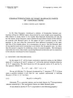
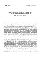
Figure 2.1: A vertex-colored poset P and an edge-colored lattice L.
(The set of vertex colors for P and the set of edge colors for L are {α, β}.
Elements of P are denoted v
i
and elements of L are denoted t
i
.)
P
s
v
6
β
s
v
5
α
s
v
4
α
s
v
3
α

s
v
2
β
s
v
1
β









❅
❅
❅
❅
❅
❅ ❅
❅
❅
L = J(P )
❅
❅
❅
❅

❅


















❅
❅
❅
❅
❅
❅
❅
❅
❅
❅
❅

❅
❅
❅









❅
❅
❅
❅
❅









❅
❅
❅
❅

❅
❅
❅
❅
❅









❅
❅
❅
❅
❅
❅
❅
❅
❅
st
0
st
1
st
2
st

3
st
4
st
5
st
6
st
7
st
8
st
9
st
10
st
11
st
12
st
13
st
14
β α
β α β β
βα α β β
α
β
β β
α

β
α αβ β
β α
Hasse diagram if and only if t covers s, i.e. s < t and there is no x in R such that
s < x < t. Thus, terminology (connected, edge-colored, dual, vertex-colored, etc) that
applies to directed graphs will also apply to posets. When we depict the Hasse diagram
for a poset, its edges are directed “up.” In an edge-colored poset R, we say the vertex s
and the edge s
i
→ t are below t, and the vertex t and the edge s
i
→ t are above s. The
vertex s is a descendant of t, and t is an ancestor of s. The edge-colored and vertex-
colored directed graphs studied in this paper will turn out to be posets. For a directed
graph R, a rank function is a surjective function ρ : R −→ {0, . . . , l} (where l ≥ 0) with
the property that if s → t in R, then ρ(s) + 1 = ρ(t); if such a rank function exists then
R is the Hasse diagram for a poset — a ranked poset. We call l the length of R with
respect to ρ, and the set ρ
−1
(i) is the ith rank of R. In an edge-colored ranked poset R,
comp
i
(t) will be a ranked poset for each t ∈ R and i ∈ I. We let l
i
(t) denote the length
of comp
i
(t), and we let ρ
i
(t) denote the rank of t within this component. We define the

depth of t in its i-component to be δ
i
(t) := l
i
(t) −ρ
i
(t).
For distributive lattices we follow the notation and language of [Sta]. In particular,
the distributive lattice of order ideals taken from a poset P (partially ordered by subset
containment) will be denoted J(P ), and we use s ∨ t and s ∧ t to denote the least upper
bound (“join”) and greatest lower bound (“meet”) respectively for two elements s and t
of the distributive lattice J(P ). If we regard the Hasse diagram for L to be an undirected
the electronic journal of combinatorics 13 (2006), #R109 5
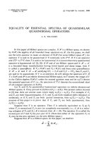
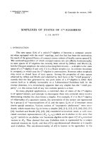
Figure 2.2: L
∗
and (L
∗
)
σ
for the lattice L from Figure 2.1.
(Here σ(α) = 1 and σ(β) = 2.)
L
∗
s
s s
s s s
s s s
s s s
s s
s❅

❅
❅
❅
❅
β





α
❅
❅
❅
❅
❅
β





α
❅
❅
❅
❅
❅
β






β





α
❅
❅
❅
❅
❅
β α





β
❅
❅
❅
❅
❅
β
α






β
❅
❅
❅
❅
❅
β





β
α
❅
❅
❅
❅
❅
β
❅
❅
❅
❅
❅

α





β α
❅
❅
❅
❅
❅
β





β
❅
❅
❅
❅
❅
α
(L
∗
)
σ
s

s s
s s s
s s s
s s s
s s
s❅
❅
❅
❅
❅
2





1
❅
❅
❅
❅
❅
2





1
❅

❅
❅
❅
❅
2





2





1
❅
❅
❅
❅
❅
2 1





2
❅

❅
❅
❅
❅
2
1





2
❅
❅
❅
❅
❅
2





2
1
❅
❅
❅
❅
❅

2
❅
❅
❅
❅
❅
1





2 1
❅
❅
❅
❅
❅
2





2
❅
❅
❅
❅
❅

1
graph, the we define the distance dist(s, t) between s and t in L to be the minimum
length achieved when all paths from s to t in L are considered; it can be seen that
dist(s, t) = 2ρ(s ∨ t) − ρ(s) − ρ(t) = ρ(s) + ρ(t) − 2ρ(s ∧ t). A coloring of the vertices
of the poset P gives a natural coloring of the edges of the distributive lattice L = J(P )
in the following way: Given a function vertexcolor
P
: V(P ) −→ I which assigns to each
vertex of P a color from the target set I, then we give a covering relation s → t in L the
color i and write s
i
→ t if t \ s = {u} and vertexcolor
P
(u) = i. So we can regard L
to be an edge-colored distributive lattice with edges colored by the set I; for brevity, we
write L = J
color
(P ). See Figure 2.4 for an example. Note that J
color
(P
∗
)
∼
=
(J
color
(P ))
∗
,
J

color
(P
σ
)
∼
=
(J
color
(P ))
σ
(recoloring), and J
color
(P ⊕Q)
∼
=
J
color
(P ) ×J
color
(Q). An edge-
colored poset P has the diamond coloring property if whenever
r
r
r
r

❅
❅
❅
❅



k
l
i
j
is an edge-colored
subgraph of the Hasse diagram for P , then i = l and j = k; a necessary and sufficient
condition for an edge-colored distributive lattice L to be isomorphic (as an edge-colored
poset) to J
color
(P ) for some vertex-colored poset P is for L to have the diamond coloring
property. For s ∈ L and i ∈ I, one can see that comp
i
(s) is the Hasse diagram for a
distributive lattice; in particular, comp
i
(s) is a distributive sublattice of L in the induced
order, and a covering relation in comp
i
(s) is also a covering relation in L.
Let n be a positive integer. We use g to denote the complex semisimple Lie algebra of
the electronic journal of combinatorics 13 (2006), #R109 6
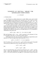
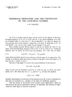
Figure 2.3: The disjoint sum of the β-components of the edge-colored lattice L from
Figure 2.1.
st
0
st
1
β

st
3
β
st
2
st
4
β
st
6
β
st
5
β
st
8
β β
st
10
β β
st
7
st
9
β
st
11
β
st
13

ββ
st
12
st
14
β


















❅
❅
❅
❅
❅
❅

❅
❅
❅






❅
❅
❅
❅
❅
❅
❅
❅
❅
  
rank n with Chevalley generators {x
i
, y
i
, h
i
}
i∈I
satisfying the Serre relations associated to
a Dynkin diagram D with n nodes; here the nodes of D are indexed by a set I of cardinality
n. We often take I = {1, . . . , n}; then our numbering of the nodes of the Dynkin diagrams

for the simple Lie algebras follows [Hum] p. 58 with the exception that for us the B
n
series
starts with n = 3 and the C
n
series with n = 2. In what follows the numbers D
i,j
and D
j,i
can be found in Figure 2.5 by looking at the subgraph of D determined by the choice of
distinct nodes i and j; set D
i,i
:= 2 for all i ∈ I. The Cartan matrix for D (or for g, when
the indexing set I and Dynkin diagram D are understood) is the matrix (D
i,j
)
(i,j)∈I×I
.
With i = 1 and j = 2, the diagrams in Figure 2.5 are Dynkin diagrams for the rank two
semisimple Lie algebras A
1
×A
1
, A
2
, C
2
, and G
2
respectively (A

2
, C
2
, and G
2
are simple).
Two Dynkin diagrams D and D

are isomorphic if under some one-to-one correspondence
σ : I −→ I

of indexing sets it is the case that D
i,j
= D

σ(i),σ(j)
and D
j,i
= D

σ(j),σ(i)
;
in this case the mapping which sends x
i
→ x

σ(i)
, y
i
→ y


σ(i)
, and h
i
→ h

σ(i)
extends
to an isomorphism of the semisimple Lie algebras g and g

with Chevalley generators
{x
i
, y
i
, h
i
}
i∈I
and {x

j
, y

j
, h

j
}
j∈I


respectively. We use {ω
i
}
i∈I
to denote the fundamental
weights corresponding to the nodes of D. The simple root α
j
(j ∈ I) can be identified
with

i∈I
D
j,i
ω
i
. We let Λ denote the lattice of weights, i.e. the set of all integral linear
combinations of the fundamental weights. Elements of Λ are called weights. Coordinatize
the lattice of weights Λ to obtain a one-to-one correspondence with Z
n
as follows: identify
ω
i
with the vector (0, . . . , 1, . . . , 0) whose only nonzero coordinate is in the ith position.
Then the simple root α
j
is identified with the jth row vector from the Cartan matrix for
g.
Vector spaces in this paper will be assumed to be complex and finite-dimensional. If
V is a g-module, then there is at least one basis B := {v

s
}
s∈R
(where R is an indexing
set with |R| = dim V ) consisting of eigenvectors for the actions of the h
i
’s: for any s in
R and i ∈ I, there exists an integer k
i
(s) such that h
i
.v
s
= k
i
(s)v
s
. The weight of the
basis vector v
s
is the sum wt(v
s
) :=

i∈I
k
i
(s)ω
i
. We say B is a weight basis for V . If µ

is a weight in Λ, then we let V
µ
be the subspace of V spanned by all basis vectors v
s
∈ B
such that wt(v
s
) = µ; V
µ
is independent of the choice of weight basis B; any nonzero v
in V
µ
is said to be a weight vector with weight µ. A nonzero vector v in V is maximal if
x
i
.v = 0 for every i ∈ I; every weight basis for V will have at least one maximal vector.
A g-module with a unique (up to scalar multiples) maximal vector v has highest weight λ
the electronic journal of combinatorics 13 (2006), #R109 7
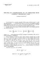
Figure 2.4: Below is the lattice L from Figure 2.1 recognized as J
color
(P ).
(The vertex-colored poset P is shown in Figure 2.1.
Each order ideal taken from P is identified by the indices of its maximal vertices.
For example, 2, 3 in L denotes the order ideal {v
2
, v
3
, v
4
, v

5
, v
6
} in P .)
L = J
color
(P )
❅
❅
❅
❅
❅



















❅
❅
❅
❅
❅
❅
❅
❅
❅
❅
❅
❅
❅
❅









❅
❅
❅
❅
❅










❅
❅
❅
❅
❅
❅
❅
❅
❅









❅
❅
❅
❅
❅

❅
❅
❅
❅
s
1, 3
s
2, 3
s
1, 6
s
3
s
2, 4, 6
s
1
s
4, 6
s
2, 6
s
2, 4
s
5, 6
s
4
s
2
s
6

s
5
s
∅
β α
β α β β
βα α β β
α
β
β β
α
β
α αβ β
β α
if v has weight λ; an irreducible module has a unique maximal vector. Finite-dimensional
irreducible g-modules are in one-to-one correspondence with dominant weights, i.e. the
nonnegative linear combinations of the fundamental weights: An irreducible g-module
corresponds to the dominant weight λ if it has highest weight λ. The Lie algebra g acts
on the dual space V
∗
by the rule (z.f)(v) = −f(z.v) for all v ∈ V , f ∈ V
∗
, and z ∈ g.
If a g-module V has weight basis B := {v
s
}
s∈R
, then form an edge-colored directed
graph on the vertex set R which indicates the supports of the actions of the generators
on the weight basis B as follows: A directed edge s

i
→ t of color i is placed from index s
to index t if c
t,s
v
t
(with c
t,s
= 0) appears as a term in the expansion of x
i
.v
s
as a linear
combination in the weight basis B, or if d
s,t
v
s
(with d
s,t
= 0) appears when we expand y
i
.v
t
in the weight basis B. The resulting edge-colored directed graph, which is also denoted
by R, is the supporting graph for the weight basis B of V , or simply a supporting graph
for V . We say an edge-colored directed graph R is a supporting graph for g if R is a
supporting graph for some representation of g. Disregarding edge colors, a supporting
graph is always the Hasse diagram for a ranked poset (Lemma 3.1.E of [Don1]). To keep
track of the actions of the generators on vectors of the weight basis B we sometimes
attach the two coefficients c

t,s
(the “x”-coefficient) and d
s,t
(the “y”-coefficient) to each
the electronic journal of combinatorics 13 (2006), #R109 8
Figure 2.5
Subgraph D
i,j
D
j,i
✉ ✉
i j
0 0
✉ ✉
i j
−1 −1
✉ ✉✟
✟
❍
❍
i j
−1 −2
✉ ✉✟
✟
❍
❍
i j
−1 −3
edge s
i

→ t of R. In this case,
x
i
.v
s
=

t:s
i
→t
c
t,s
v
t
and y
i
.v
t
=

s:s
i
→t
d
s,t
v
s
. (1)
The supporting graph R together with the coefficients {(c
t,s

, d
s,t
)}
s
i
→t∈E(R)
is the represen-
tation diagram (also denoted by R) for the weight basis B of V . If the coefficients c
t,s
and
d
s,t
are positive rational numbers (respectively, positive integers), then we say that the
weight basis B is positive rational (respectively positive integral). A supporting graph R of
V is positive rational (resp. positive integral) if there is a positive rational (resp. positive
integral) weight basis for V which has R as its supporting graph. We say R is a modular
lattice (respectively, distributive lattice) supporting graph if R is a modular lattice (resp.
distributive lattice) when viewed as the Hasse diagram for a poset. A supporting graph R
for a weight basis B of V is edge-minimal if no other weight basis for V has its supporting
graph appearing as a proper edge-colored subgraph of R; the supporting graph R is edge-
minimizing if no other weight basis for V has a supporting graph with fewer edges than
R. In a sense, then, an edge-minimal supporting graph is locally edge-minimizing. Two
weight bases {v
s
}
s∈R
and {w
t
}
t∈Q

for V are diagonally equivalent if there is an ordering
on these bases with respect to which the corresponding change of basis matrix is diagonal;
the bases are scalar equivalent if this diagonal matrix is a scalar multiple of the identity.
The supporting graph for the weight basis B is solitary if no weight basis for V has the
same supporting graph as B other than those weight bases that are diagonally equivalent
to B. Observe that, up to diagonal equivalence, a representation can have at most a finite
number of solitary bases. The adjectives modular (or distributive) lattice, edge-minimal,
edge-minimizing, and solitary apply to weight bases as well as supporting graphs. Up
to diagonal equivalence, then, a solitary weight basis is uniquely identified by its sup-
porting graph. Figure 5.2 depicts the representation diagram for a weight basis for the
“adjoint” representation of G
2
; this basis is positive rational, solitary, and edge-minimal
(cf. Theorem 5.1 and Proposition 5.4).
Let R be a ranked poset whose Hasse diagram edges are colored with colors taken from
a set I of cardinality n. For i ∈ I and s in R, set m
i
(s) := ρ
i
(s) − δ
i
(s) = 2ρ
i
(s) − l
i
(s).
Let wt
R
(s) be the n-tuple ( m
i

(s) )
i∈I
. Given a matrix M = (M
p,q
)
(p,q)∈I×I
, then for fixed
i ∈ I let M
(i)
be the n-tuple (M
i,j
)
j∈I
, the ith row vector for M. We say R satisfies the
structure condition for M if wt
R
(s) + M
(i)
= wt
R
(t) whenever s
i
→ t for some i ∈ I,
that is, for all j ∈ I we have m
j
(s) + M
i,j
= m
j
(t). (In [Don3] it is shown that M must

the electronic journal of combinatorics 13 (2006), #R109 9
in fact be a Cartan matrix if the edge color function is surjective.) Following [DLP1],
we say R satisfies the g-structure condition if M is the Cartan matrix for the Dynkin
diagram D associated to g. In this case view wt
R
: R −→ Λ as the function given by
wt
R
(s) =

j∈I
m
j
(s)ω
j
. Then R satisfies the g-structure condition if and only if for each
simple root α
i
we have wt
R
(s) + α
i
= wt
R
(t) whenever s
i
→ t in R. (In [Don1] the edges
of R in this case were said to “preserve weights.”) This condition depends not only on
g (information from the corresponding Dynkin diagram) but also on the combinatorics
of R. The edge-colored distributive lattice of Figure 2.6 satisfies the structure condition

for the matrix M =

2 −1
−1 2

and therefore satisfies the A
2
-structure condition. The
following simple lemma merely observes when the matrix M is uniquely determined by
an edge-colored ranked poset R that satisfies some structure condition.
Figure 2.6: For each element t of the lattice L from Figure 2.1, we compute
wt
L
(t) = (m
α
(t), m
β
(t)).
❅
❅
❅
❅
❅



















❅
❅
❅
❅
❅
❅
❅
❅
❅
❅
❅
❅
❅
❅










❅
❅
❅
❅
❅









❅
❅
❅
❅
❅
❅
❅
❅
❅










❅
❅
❅
❅
❅
❅
❅
❅
❅
s
(1, 2)
s
(2, 0)
s
(−1, 3)
s
(3, −2)
s
(0, 1)
s
(0, 1)
s
(1, −1)
s

(−2, 2)
s
(1, −1)
s
(−1, 0)
s
(2, −3)
s
(−1, 0)
s
(−3, 1)
s
(0, −2)
s
(−2, −1)
β α
β α β β
βα α β β
α
β
β β
α
β
α αβ β
β α
Lemma 2.1 Let R be a ranked poset with edges colored by a set I. Suppose the edge
coloring function edgecolor
R
: E(R) −→ I is surjective. (1) Suppose R satisfies the
structure condition for matrices M = (M

i,j
)
(i,j)∈I×I
and M

= (M

i,j
)
(i,j)∈I×I
. Then for all
i, j ∈ I, M
i,j
= M

i,j
, and this quantity is an integer. Moreover, M
i,i
= 2 for all i ∈ I. (2)
Let D and D

be two Dynkin diagrams whose nodes are indexed by I, and let g and g

be
the corresponding semisimple Lie algebras. If R satisfies the g-structure and g

-structure
conditions, then D and D

are isomorphic under the correspondence given by I, and hence

g
∼
=
g

.
the electronic journal of combinatorics 13 (2006), #R109 10
Proof. (2) follows from (1). For (1), note that for each j ∈ I there is an edge s
j
→ t
in R. Then for each i ∈ I, M
j,i
= m
i
(t) − m
i
(s) = M

j,i
. When i = j, note that
ρ
i
(t) = ρ
i
(s) + 1 and l
i
(s) = l
i
(t), so 2 = m
i

(t) −m
i
(s).
An edge-labelled poset R with colors from I is an edge-colored ranked poset R with edge
colors from the set I together with an assignment of edge coefficients {(c
t,s
, d
s,t
)}
s
i
→t∈E(R)
.
In the ordered pair (c
t,s
, d
s,t
), we think of c
t,s
as an x-coefficient and d
s,t
as a y-coefficient.
We call π
s,t
:= c
t,s
d
s,t
the edge product associated to a given edge s
i

→ t in the edge-labelled
poset R. If σ : I → I

is a mapping of sets, then we regard the recoloring R
σ
of R to be
an edge-labelled poset where the coefficients assigned to an edge s
σ(i)
−→ t in R
σ
are the
same as the coefficients assigned to the edge s
i
→ t in R. Make the edge-colored poset R
∗
an edge-labelled poset as follows: Give an edge t
∗
i
→ s
∗
in R
∗
coefficients c
s
∗
,t
∗
:= d
s,t
and

d
t
∗
,s
∗
:= c
t,s
, where the edge s
i
→ t in R has x- and y-coefficients c
t,s
and d
s,t
respectively.
The set {(c
t,s
, d
s,t
)}
s
i
→t∈E(R)
of coefficients is nonzero if π
s,t
= 0 for all edges s
i
→ t in
E(R). The edge-labelled poset R satisfies the crossing condition if for any s in R and any
color i ∈ I, we have


r:r
i
→s
π
r,s
−

t:s
i
→t
π
s,t
= m
i
(s). (2)
A relation of form (2) is a crossing relation. The edge-labelled poset R satisfies the
diamond condition if for any pair of vertices s and t in R and any colors i and j in I, we
have

u: s
j
→u and t
i
→u
c
u,s
d
t,u
=


r: r
i
→s and r
j
→t
d
r,s
c
t,r
, (3)
where an empty sum is zero. Suppose there is a unique element u such that s
j
→ u and
t
i
→ u, and suppose there is a unique element r such that r
i
→ s and r
j
→ t. Then we
have this subgraph in R:
r
r
r
r

❅
❅
❅
❅



j
i
i
j
r
s
u
t
.
The diamond condition in this case implies that:
c
u,s
d
t,u
= d
r,s
c
t,r
and c
u,t
d
s,u
= d
r,t
c
s,r
(4)
and

π
s,u
π
t,u
= π
r,s
π
r,t
. (5)
Any relation of the form (3), (4), or (5) is a diamond relation. We let V [R] be the complex
vector space with basis {v
s
}
s∈R
, and for i ∈ I, we let x
i
and y
i
act on V [R] using the
identities at (1) above. The following proposition is a reformulation of Proposition 3.4 of
[Don1]. As an example, one can apply this result to the edge-labelled poset of Figure 5.2
to see that it is a representation diagram for some representation of G
2
.
Proposition 2.2 Let D be a Dynkin diagram whose nodes are indexed by a set I, and
let g be the associated semisimple Lie algebra with Chevalley generators {x
i
, y
i
, h

i
}
i∈I
.
Let R be an edge-labelled poset with colors from I having the property that at least one
the electronic journal of combinatorics 13 (2006), #R109 11
of the two coefficients (c
t,s
or d
s,t
) assigned to any given edge s
i
→ t in P is nonzero. Then
V [R] is a g-module (with the action of g induced by the actions on V [R] of the x
i
’s and
y
i
’s as described at (1) above) and the edge-labelled poset R is a representation diagram
for the weight basis {v
s
}
s∈R
of V [R] if and only if R satisfies the diamond, crossing,
and g-structure conditions. In this case, h
i
.v
s
= m
i

(s)v
s
for any s in R and i ∈ I, so
wt(v
s
) =

i∈I
m
i
(s)ω
i
= wt
R
(s).
Lemma 2.3 Suppose R is the representation diagram for some weight basis of a g-module
V . Then the edge-labelled poset R
∗
is a representation diagram for the dual representation
V
∗
of g. Moreover, the edge-colored poset R
∗
is a positive rational (respectively positive
integral, modular (or distributive) lattice, solitary, edge-minimal, edge-minimizing) sup-
porting graph for V
∗
if R is positive rational (respectively positive integral, modular (or
distributive) lattice, solitary, edge-minimal, edge-minimizing).
Proof. It is easy to see that the edge-labelled poset R

∗
satisfies the diamond, crossing,
and g-structure conditions, and hence by Proposition 2.2 it is a representation diagram
for some representation of g. By Lemma 3.3.A of [Don1], this representation is isomorphic
to V
∗
. Clearly the edge coefficients attached to R
∗
are all positive rational (respectively
positive integral) if the coefficients for R are positive rational (resp. positive integral).
The poset-dual of a modular (or distributive) lattice is also a modular (or distributive)
lattice.
The remaining claims of the lemma can be proved by contrapositive. This is effected
by the following observation: The poset (R
∗
)
∗
is isomorphic to R as an edge-colored
poset via the correspondence of vertices x
∗∗
→ x; then corresponding edges of the edge-
labelled posets R and (R
∗
)
∗
have identical edge coefficients. So suppose R
∗
contains as
a proper edge-colored subposet some supporting graph Q
∗

for V
∗
where Q is a proper
edge-colored subposet of R. Then Q is a supporting graph for V
∼
=
(V
∗
)
∗
since (Q
∗
)
∗
is a supporting graph for (V
∗
)
∗
and Q
∼
=
(Q
∗
)
∗
. Thus R contains as a proper edge-
colored subposet a supporting graph Q for V . That is, if R
∗
is not edge-minimal, then
R is not edge-minimal. It is similarly easy to show that if R

∗
is not edge-minimizing,
then R is not edge-minimizing. Now suppose that R
∗
is not solitary as a supporting
graph for V
∗
. Then if {v
t
∗
}
t
∗
∈R
∗
denotes a weight basis for V
∗
whose representation
diagram is the edge-labelled poset R
∗
, there must be another weight basis {w
t
∗
}
t
∗
∈R
∗
for
V

∗
with supporting graph R
∗
and such that {v
t
∗
} and {w
t
∗
} are not diagonally equivalent.
Write w
t
∗
=

s
∗
∈R
∗
a
s
∗
,t
∗
v
s
∗
, so that the scalars (a
s
∗

,t
∗
)
(s
∗
,t
∗
)∈R
∗
×R
∗
describe the change of
basis. Now let {u
t
}
t∈R
be a weight basis for V with representation diagram R. Set
z
t
:=

s∈R
a
s
∗
,t
∗
u
t
. Then {z

t
}
t∈R
is a weight basis for V that is not diagonally equivalent
to {u
t
}
t∈R
but has supporting graph R.
The following (obvious) lemma follows from the definitions but is useful as a principle,
particularly when the Dynkin diagram has symmetry (A
n
, D
n
, and E
6
) or when other
numberings of the Dynkin diagram are convenient.
Lemma 2.4 Let D and D

be Dynkin diagrams with nodes indexed by I and I

respec-
tively such that D and D

are isomorphic under a one-to-one correspondence σ : I −→ I

.
the electronic journal of combinatorics 13 (2006), #R109 12
Let g and g


be the respective semisimple Lie algebras. Let R be a ranked poset with
edges colored by the set I, and consider the recoloring R
σ
. Then R is a supporting graph
for g (respectively, positive integral, positive rational, modular (or distributive) lattice,
solitary, edge-minimal, or edge-minimizing support) if and only if R
σ
is a supporting
graph for g

(respectively, positive integral, positive rational, modular (or distributive)
lattice, solitary, edge-minimal, or edge-minimizing support).
Lemmas 2.3 and 2.4 can work in tandem as follows. For any Dynkin diagram D there
is a special permutation σ
0
of the index set I that yields a symmetry of the Dynkin
diagram. See the discussion in Section 2 of [ADLMPW]. For A
2
with index set {1, 2}, we
have σ
0
(1) = 2 and σ
0
(2) = 1; for A
1
× A
1
, C
2

, and G
2
, σ
0
is trivial. Here we extend the
notion of the “” operation from [ADLMPW] on edge-colored and vertex-colored posets
to an operation on edge-labelled posets as follows: Given a representation diagram R for
a representation V of g, we let R

be the edge-labelled poset (R
∗
)
σ
0
and call R

the
σ
0
-recolored dual of R. That is, take the edge-labelled poset R
∗
and recolor the edges by
applying σ
0
as in Lemma 2.4 to obtain (R
∗
)
σ
0
. Observe that (R


)

= R. For an example,
see Figure 2.7.
Figure 2.7: L

for the lattice L from Figure 2.1.
(In Theorem 5.1 we see that the edge-colored lattice L is a supporting graph
for A
2
with Dynkin diagram s
α
s
β
.)
s
s s
s s s
s s s
s s s
s s
s❅
❅
❅
❅
❅
α






β
❅
❅
❅
❅
❅
α





β
❅
❅
❅
❅
❅
α





α






β
❅
❅
❅
❅
❅
α β





α
❅
❅
❅
❅
❅
α
β





α
❅

❅
❅
❅
❅
α





α
β
❅
❅
❅
❅
❅
α
❅
❅
❅
❅
❅
β





α β

❅
❅
❅
❅
❅
α





α
❅
❅
❅
❅
❅
β
Proposition 2.5 In the notation of the preceding paragraph, the edge-labelled poset R

is also a representation diagram for the g-module V . Moreover, the edge-colored poset
R

is a positive rational (respectively positive integral, modular (or distributive) lattice,
the electronic journal of combinatorics 13 (2006), #R109 13
solitary, edge-minimal, edge-minimizing) supporting graph for V if R is positive rational
(respectively positive integral, modular (or distributive) lattice, solitary, edge-minimal,
edge-minimizing).
Proof. The only assertion that does not immediately follow from Lemmas 2.3 and 2.4
is that R


is a supporting graph for the g-module V . But this follows from Lemma 2.2
of [ADLMPW].
3. Grid posets; two-color grid posets; semistandard
posets and lattices
Following [ADLMPW], given a finite poset (P, ≤
P
), a chain function for P is a function
chain : P −→ {1, 2, . . . , m} for some positive integer m such that (1) C
i
:= chain
−1
(i) is a
(possibly empty) chain in P for 1 ≤ i ≤ m, and (2) given any covering relation u → v in P ,
it is the case that either chain(u) = chain(v) or chain(u) = chain(v)+1. A grid poset is
a finite poset (P, ≤
P
) together with a chain function chain : P −→ {1, 2, . . . , m} for some
positive integer m. We let T
P
be the totally ordered set whose elements are the elements of
P and whose ordering is given by the following rule: for distinct u and v in P write u <
T
P
v
if and only if (1) chain(u) < chain(v) or (2) chain(u) = chain(v) with v <
P
u. Let
l := |P |. Number the vertices of P v
1

, v
2
, . . . , v
l
so that v
p
<
T
P
v
q
whenever 1 ≤ p < q ≤ l.
Let L := J(P ) be the distributive lattice of order ideals taken from P . We simultaneously
think of order ideals taken from P as subsets of P and as elements of L. Let m be the
maximal element of L (so as sets, m = P ). For 1 ≤ i ≤ l, set b
i
:= P \{v
1
, . . . , v
i
}, and set
b
0
:= m; observe that each b
i
is an order ideal taken from P . The sequence of order ideals
(b
0
, b
1

, ···, b
l
) is the boundary of L. Let ρ : L −→ {0, . . . , l} denote the rank function of
L. Then b
i
is the unique boundary element in the set ρ
−1
(l −i). If s → t is an edge in L,
then necessarily t\s = {v} for some v in P . Associate to L the following ancestor function
(cf. [DLP2]): ancestor
L
: L \ {m} −→ L is given by the rule ancestor
L
(s) = s ∪ {v
p
}
where v
p
is the largest element in T
P
such that v
p
∈ s and s ∪ {v
p
} ∈ L. We assign to
any given element s in L the coordinates coord(s) := (s
1
, . . . , s
m
), where s

i
is |C
i
∩ s|.
For 1 ≤ i ≤ m, let c
i
:= |C
i
|; then coord(m) = (c
1
, . . . , c
m
). If s is a descendant of t
in L where t has coordinates coord(t) = (t
1
, . . . , t
m
), then for some i with 1 ≤ i ≤ m
we have coord(s) = (t
1
, . . . , t
i−1
, t
i
− 1, t
i+1
, . . . , t
m
); we use the notation t
(i)

to refer
to this particular descendant of t. Define a total ordering T
L
on the elements of L as
follows: for distinct s and t in L, write s <
T
L
t if and only if (1) ρ(s) > ρ(t); or (2)
ρ(s) = ρ(t) and dist(s, b) < dist(t, b), where b is the unique boundary element of L for
which ρ(b) = ρ(s) = ρ(t); or (3) ρ(s) = ρ(t), dist(s, b) = dist(t, b), and there exists a j
such that s
j
> t
j
while s
i
= t
i
for i > j.
Lemma 3.1 Let P be a grid poset as above, and let s and t be elements of L = J(P )
with coord(s) = (s
1
, . . . , s
m
) and coord(t) = (t
1
, . . . , t
m
) . Then:
(1) coord(s ∨ t) =


max(s
1
, t
1
), . . . , max(s
m
, t
m
)

and coord(s ∧ t) =

min(s
1
, t
1
), . . . , min(s
m
, t
m
)

.
the electronic journal of combinatorics 13 (2006), #R109 14
(2) dist(s, t) =
m

i=1
|s

i
− t
i
|.
(3) Suppose t
(i)
and t
(j)
are descendants of t in L with i < j. Let b be the unique bound-
ary element with the same rank as t
(i)
and t
(j)
. Then dist(t
(i)
, b) ≤ dist(t
(j)
, b)
and t
(i)
<
T
L
t
(j)
.
(4) Suppose s → t in L, and let t

:= ancestor
L

(s). If t

= t, then t

<
T
L
t.
Proof. Part (1) follows immediately from the definitions. For part (2), first observe
that the rank of s in L is ρ(s) =

m
i=1
s
i
. Now apply part (1) together with the fact that
dist(s, t) = 2ρ(s ∨ t) − ρ(s) − ρ(t) = ρ(s) + ρ(t) − 2ρ(s ∧ t). For part (3), it suffices to
show that dist(t
(i)
, b) ≤ dist(t
(j)
, b). Write coord(t
(k)
) = (t
(k)
1
, . . . , t
(k)
m
) if k is i or j,

and write coord(b) = (0, . . . , 0, b
p
, c
p+1
, . . . , c
m
). Then t
(i)
i
= t
i
−1, t
(i)
j
= t
j
, t
(j)
i
= t
i
, and
t
(j)
j
= t
j
−1. From (2) we have dist(t
(i)
, b) = t

(i)
1
+ ···+ t
(i)
p−1
+ |b
p
−t
(i)
p
|+ (c
p+1
−t
(i)
p+1
) +
···+ (c
m
−t
(i)
m
) and a similar expression for dist(t
(j)
, b). Then dist(t
(j)
, b) −dist(t
(i)
, b)
=














t
(j)
i
− t
(i)
i
+ t
(j)
j
− t
(i)
j
if i < j < p
c
i
− t
(j)
i

− (c
i
− t
(i)
i
) + c
j
− t
(j)
j
− (c
j
− t
(i)
j
) if p < i < j
t
(j)
i
− t
(i)
i
+ c
j
− t
(j)
j
− (c
j
− t

(i)
j
) if i < p < j
t
(j)
i
− t
(i)
i
+ |b
p
− t
(j)
p
| −|b
p
− t
(i)
p
| if i < p, j = p
|b
p
− t
(j)
p
| − |b
p
− t
(i)
p

|+ c
j
− t
(j)
j
− (c
j
− t
(i)
j
) if i = p, p < j
=











t
i
− (t
i
− 1) + t
j
− 1 − t

j
= 0 if i < j < p
c
i
− t
i
− (c
i
− (t
i
− 1)) + c
j
− (t
j
− 1) − (c
j
− t
j
) = 0 if p < i < j
t
i
− (t
i
− 1) + c
j
− (t
j
− 1) − (c
j
− t

j
) = 2 if i < p < j
t
i
− (t
i
− 1) + |b
p
− (t
p
− 1)|−|b
p
− t
p
| = 0 or 2 if i < p, j = p
|b
p
− t
p
| − |b
p
− (t
p
− 1)| + c
j
− (t
j
− 1) − (c
j
− t

j
) = 0 or 2 if i = p, p < j
For (4), note that for some 1 ≤ p ≤ m, coord(t) = (s
1
, . . . , s
p−1
, s
p
+ 1, s
p+1
, . . . , s
m
).
Moreover, we have coord(t

) = (s
1
, . . . , s
q−1
, s
q
+ 1, s
q+1
, . . . , s
m
) for some q = p since
t

= t. By definition of ancestor
L

, it follows that q > p. Let u be the least upper bound
of t and t

in L. Then coord(u) = (s
1
, . . . , s
p
+ 1, . . . , s
q
+ 1, . . ., s
m
). When we view the
descendants t

= u
(p)
and t = u
(q)
of u in the light of part(3), then we see that t

<
T
L
t.
A two-color function for a grid poset (P, ≤
P
, chain : P −→ {1, 2, . . . , m}) is a function
color : P −→ ∆ such that (1) |∆| = 2, (2) color(u) = color(v) if chain(u) = chain(v),
and (3) if u and v are in the same connected component of P with chain(u) = chain(v)+1,
then color(u) = color(v). A two-color grid poset is a grid poset (P, ≤

P
, chain : P −→
{1, . . . , m}) together with a two-color function color : P −→ ∆. A two-color grid poset
should be thought of as a certain kind of vertex-colored poset. We will associate to a
two-color grid poset P the edge-colored distributive lattice L := J
color
(P ). We say a
two-color grid poset P has the max property if P is isomorphic to a two-color grid poset
(Q, ≤
Q
, chain : Q −→ {1, 2, . . . , m}, color : Q −→ ∆) with a surjective chain function
the electronic journal of combinatorics 13 (2006), #R109 15
such that (1) if u is any maximal element in the poset Q, then chain(u) ≤ 2, and (2) if
v = u is another maximal element in Q, then color(u) = color(v). We will often take
∆ := {α, β}. When we switch (or reverse) the vertex colors of P we replace the color
function color : P −→ {α, β} with the color function color

: P −→ {α, β} given by:
color

(v) = α if color(v) = β, and color

(v) = β if color(v) = α. Similarly, one can
switch (or reverse) the edge colors of L. In Figures 3.3 and 3.4 we depict eight two-color
grid posets with the max property; the numbering of the vertices for each poset P follows
the total ordering T
P
. The vertex-colored poset P of Figure 2.1 is a two-color grid poset
with the max property. The lattice L in that figure is J
color

(P ); the total ordering T
L
is indicated by the indices of the elements of L so that t
0
<
T
L
t
1
<
T
L
··· <
T
L
< t
14
.
The boundary is the sequence (t
0
, t
1
, t
3
, t
6
, t
9
, t
12

, t
14
). The order ideals corresponding to
elements of the lattice are depicted in Figure 2.4.
Lemma 3.2 Suppose (P, ≤
P
, chain : P −→ {1, . . . , m}, color : P −→ {α, β}) is a
two-color grid poset with the max property. Let t ∈ L = J
color
(P ). For γ ∈ {α, β}, let
t
(i
1
)
, . . . , t
(i
k
)
with 1 ≤ i
1
< ··· < i
k
≤ m be all of the descendants of t in L for which
t
(i
p
)
γ
→ t, where 1 ≤ p ≤ k. Then ancestor
L

(t
(i
p
)
) = t for 1 ≤ p < k.
In the language of [DLP2], when a two-color grid poset P has the max property,
Lemma 3.2 implies that L = J
color
(P ) together with the total ordering T
L
and ancestor
function ancestor
L
will have no “exceptional descendants” and, in light of part (4) of
Lemma 3.1, will be “diamond-and-crossing friendly.” These are the crucial facts needed
in order to apply Theorem 4.1 of [DLP2] in the proof of Theorem 4.4.
Proof of Lemma 3.2. Without loss of generality we may assume that chain is surjec-
tive. Suppose 1 ≤ p < k. Let s := t
(i
p
)
. For i
p
+ 1 ≤ j ≤ m, C
j
\s = C
j
\t. We claim that
for some j with i
p

+ 1 ≤ j ≤ m, it is the case that C
j
\ s = ∅. Otherwise, suppose that
C
j
\ s = ∅ for all i
p
+ 1 ≤ j ≤ m. We let u be the unique vertex in chain C
i
k
for which
{u} = t \ t
(i
k
)
. If u → u

for some u

in C
i
k
−1
, then since i
p
+ 1 ≤ i
k
− 1 and therefore
t ∩C
i

k
−1
= C
i
k
−1
, it follows that u

∈ t. But then t
(i
k
)
= t \{u} will not be an order ideal.
Use similar reasoning to see that there is no u

in C
i
k
for which u → u

. Therefore u is
maximal in P . Now 1 ≤ i
p
< i
k
. If i
k
> 2, then we have a maximal vertex in P which is
not in C
1

∪ C
2
, contradicting the fact that P has the max property. If i
k
= 2, then since
the chains C
i
p
and C
i
k
have the same color, it must be the case that chains C
1
and C
2
are in
different connected components of P . In particular, C
1
will be in a connected component
of its own. Then there will be at least two maximal vertices of color γ. But again this
contradicts the fact that P has the max property. So now let j be the largest integer for
which i
p
+ 1 ≤ j ≤ m and C
j
\s = C
j
\t = ∅. Let v be the largest element in T
P
for which

v ∈ C
j
\s. In particular, v is the largest element in T
P
that is not in s. If w → v for some
w ∈ P , then either w ∈ s ∩ C
j
or w ∈ C
j+1
. In either case, w ∈ s. Therefore s ∪ {v} is an
order ideal taken from P , and so ancestor
L
(s) = s ∪ {v} = t.
The converse of Lemma 3.2 formulated in Lemma 3.3 says that whenever P is a
two-color grid poset without the max property, then L = J
color
(P ) will have exceptional
descendants. Since Lemma 3.3 is not needed elsewhere in this paper, we state the result
without proof.
Lemma 3.3 Let (P, ≤
P
, chain : P −→ {1, . . . , m}, color : P −→ {α, β}) be a two-color
the electronic journal of combinatorics 13 (2006), #R109 16
grid poset without the max property. Then there exists a color γ ∈ {α, β} and an element
t of L = J
color
(P ) with two descendants r and s such that r
γ
→ t, s
γ

→ t, r precedes s in
the total order T
L
, and ancestor
L
(r) = t.
For more on the following discussion of “decomposing” grid posets and two-color grid
posets, see [ADLMPW]. Let P be a grid poset with chain function chain : P −→
{1, 2, . . . , m}. Suppose P
1
is a nonempty order ideal and is a proper subset of P . Regard
P
1
and P
2
:= P \ P
1
to be subposets of the poset P in the induced order. Suppose
that whenever u is a maximal (respectively minimal) element of P
1
and v is a maximal
(respectively minimal) element of P
2
, then chain(u) ≤ chain(v). Then we say that P
decomposes into P
1
 P
2
, and we write P = P
1

 P
2
. If no such order ideal P
1
exists, then
we say the grid poset P is indecomposable. If P is a grid poset that decomposes into
P
1
 Q, and if Q decomposes into P
2
 P
3
, then P = P
1
 (P
2
 P
3
). But now observe
that P = (P
1
 P
2
)  P
3
. So we may write P = P
1
 P
2
 P

3
unambiguously. In general,
if P = P
1
 P
2
 ···  P
k
, then each P
i
with chain function chain|
P
i
is a grid subposet of
P . If in addition P is a two-color grid poset with two-color function color, then each P
i
with chain function chain|
P
i
and two-color function color|
P
i
is a two-color grid subposet
of P , and so P
1
 P
2
 ··· P
k
is a decomposition of P into two-color grid posets.

For the remainder of this paper, we let g denote a rank two semisimple Lie algebra,
we identify α with a short simple root for g, and we identify β as the other simple root.
The vertex colors and edge colors for the posets and lattices we now present are simple
roots. Let ω
α
= ω
1
= (1, 0) and ω
β
= ω
2
= (0, 1) respectively denote the corresponding
fundamental weights. Any weight µ in Λ of the form µ = pω
α
+ qω
β
(where p and q are
integers) is now identified with the pair (p, q) in Z × Z. Then α and β are respectively
identified with the first and second row vectors from the Cartan matrix for g:
Figure 3.1
A
1
× A
1

2 0
0 2

A
2


2 −1
−1 2

C
2

2 −1
−2 2

G
2

2 −1
−3 2

In this notation, we define the g-fundamental posets P
g
(1, 0) and P
g
(0, 1) to be the two-
color grid posets of Figure 3.2. The corresponding g-fundamental lattices are the edge-
colored lattices L
g
(1, 0) := J
color
(P
g
(1, 0)) and L
g

(0, 1) := J
color
(P
g
(0, 1)) respectively.
Now let λ = (a, b) be a pair of nonnegative integers. There are exactly two possible ways
that a two-color grid poset P with the max property can decompose as P
1
 P
2
 ··· P
a+b
with a of the P
i
’s vertex-color isomorphic to P
g
(1, 0) and the remaining P
i
’s vertex-color
isomorphic to P
g
(0, 1): we will either have P
i
isomorphic to P
g
(0, 1) for 1 ≤ i ≤ b and
isomorphic to P
g
(1, 0) for 1 + b ≤ i ≤ a + b (in which case we set P
βα

g
(λ) := P ), or we will
have P
i
isomorphic to P
g
(1, 0) for 1 ≤ i ≤ a and isomorphic to P
g
(0, 1) for a+1 ≤ i ≤ a+b
(in which case we set P
αβ
g
(λ) := P ). Note that P
βα
g
(1, 0) = P
αβ
g
(1, 0) = P
g
(1, 0), and
P
βα
g
(0, 1) = P
αβ
g
(0, 1) = P
g
(0, 1). When a = b = 0, then P

βα
g
(λ) and P
αβ
g
(λ) are the
empty set. We call P
βα
g
(λ) and P
αβ
g
(λ) the g-semistandard posets associated to λ. For
the electronic journal of combinatorics 13 (2006), #R109 17
each semisimple Lie algebra g, P
βα
g
(2, 2) is depicted in Figure 3.3; P
αβ
g
(2, 2) is depicted
in Figure 3.4. The g-semistandard lattices associated to λ are the edge-colored lattices
L
βα
g
(λ) := J
color
(P
βα
g

(λ)) and L
αβ
g
(λ) := J
color
(P
αβ
g
(λ)). Note that L
βα
g
(1, 0) = L
αβ
g
(1, 0) =
L
g
(1, 0), and L
βα
g
(0, 1) = L
αβ
g
(0, 1) = L
g
(0, 1).
Figure 3.2: Fundamental posets.
Algebra g P
g
(1, 0) P

g
(0, 1)
A
1
× A
1
v
1
s α
v
1
s β
A
2
v
2
s
β
v
1
s
α
❅
❅
❅
v
2
s
α
v

1
s
β
❅
❅
❅
C
2
v
3
s
α
v
2
s
β
v
1
s
α
❅
❅
❅
❅
❅
❅
v
4
s
β

v
3
s
α
v
2
s
α
v
1
s
β



❅
❅
❅
❅
❅
❅
G
2
v
6
s
α
v
5
s

β
v
4
s
α
v
3
s
α
v
2
s
β
v
1
s
α



❅
❅
❅
❅
❅
❅
❅
❅
❅
❅

❅
❅
v
10
s
β
v
9
s
α
v
8
s
α
v
6
s
β v
7
s
α
v
4
s
α v
5
s
β
v
3

s
α
v
2
s
α
v
1
s
β















❅
❅
❅
❅
❅

❅
❅
❅
❅
❅
❅
❅
❅
❅
❅
❅
❅
❅
the electronic journal of combinatorics 13 (2006), #R109 18
Figure 3.3: Depicted below are four two-color grid posets each possessing the max property.
(Each is the g-semistandard poset P
βα
g
(2, 2) for the indicated rank two semisimple Lie algebra g.)
g = A
1
× A
1
s
v
4
α
s
v
3

α
s
v
2
β
s
v
1
β






C
1
C
2

g = A
2
s
v
8
β
s
v
7
β

s
v
6
α
s
v
5
α
s
v
4
α
s
v
3
α
s
v
2
β
s
v
1
β
















❅
❅
❅
❅
❅
❅ ❅
❅
❅
❅
❅
❅
C
1
C
2
C
3
g = C
2
s
v

14
α
s
v
13
α
s
v
12
β
s
v
11
β
s
v
10
β
s
v
9
β
s
v
8
α
s
v
7
α

s
v
6
α
s
v
5
α
s
v
4
α
s
v
3
α
s
v
2
β
s
v
1
β









































❅
❅
❅
❅
❅
❅
❅
❅
❅
❅
❅
❅ ❅
❅
❅
❅
❅
❅
❅
❅
❅
❅
❅
❅
C
1
C
2

C
3
C
4
g = G
2
s
v
30 β
s
v
26
α
s
v
25
α
s
v
16
β
s
v
24
α
s
v
29
β
s

v
10
α
s
v
15
β
s
v
23
α
s
v
9
α
s
v
22
α
s
v
32
α
s
v
8
α
s
v
14

β
s
v
21
α
s
v
28
β
s
v
2
β
s
v
7
α
s
v
13
β
s
v
20
α
s
v
31
α
s

v
6
α
s
v
19
α
s
v
27
β
s
v
5
α
s
v
12
β
s
v
18
α
s
v
1
β
s
v
4

α
s
v
17
α
s
v
11
β
s
v
3
α


















































































































❅
❅
❅
❅
❅
❅
❅
❅
❅
❅
❅
❅
❅
❅
❅
❅
❅
❅
❅
❅
❅
❅
❅
❅
❅
❅
❅

❅
❅
❅
❅
❅
❅
❅
❅
❅
❅
❅
❅
❅
❅
❅
❅
❅
❅
❅
❅
❅
❅
❅
❅
❅
❅
❅
❅
❅
❅

❅
❅
❅
C
6
C
5
C
4
C
3
C
2
C
1
the electronic journal of combinatorics 13 (2006), #R109 19
Figure 3.4: Depicted below are four two-color grid posets each possessing the max property.
(Each is the g-semistandard poset P
αβ
g
(2, 2) for the indicated rank two semisimple Lie algebra g.)
g = A
1
× A
1
s
v
4
β
s

v
3
β
s
v
2
α
s
v
1
α






C
1
C
2

g = A
2
s
v
8
α
s
v

7
α
s
v
6
β
s
v
5
β
s
v
4
β
s
v
3
β
s
v
2
α
s
v
1
α
















❅
❅
❅
❅
❅
❅ ❅
❅
❅
❅
❅
❅
C
1
C
2
C
3
g = C
2

s
v
1
α
s
v
2
α
s
v
3
β
s
v
4
β
s
v
5
β
s
v
6
β
s
v
7
α
s
v

8
α
s
v
9
α
s
v
10
α
s
v
11
α
s
v
12
α
s
v
13
β
s
v
14
β









































❅
❅
❅
❅
❅
❅
❅
❅
❅
❅
❅
❅
❅
❅
❅
❅
❅
❅
❅
❅
❅
❅
❅
❅
C

1
C
2
C
3
C
4
g = G
2
s
v
1
α
s
v
2
α
s
v
3
β
s
v
4
β
s
v
5
β
s

v
6
β
s
v
7
α
s
v
8
α
s
v
9
α
s
v
10
α
s
v
11
α
s
v
12
α
s
v
13

α
s
v
14
α
s
v
15
α
s
v
16
α
s
v
17
β
s
v
18
β
s
v
19
β
s
v
20
β
s

v
21
β
s
v
22
β
s
v
23
α
s
v
24
α
s
v
25
α
s
v
26
α
s
v
27
α
s
v
28

α
s
v
29
α
s
v
30
α
s
v
31
β
s
v
32
β


















































































































❅
❅
❅
❅
❅
❅
❅
❅
❅
❅
❅
❅
❅
❅
❅
❅
❅
❅
❅
❅
❅
❅
❅

❅
❅
❅
❅
❅
❅
❅
❅
❅
❅
❅
❅
❅
❅
❅
❅
❅
❅
❅
❅
❅
❅
❅
❅
❅
❅
❅
❅
❅
❅

❅
❅
❅
❅
❅
❅
❅
C
6
C
5
C
4
C
3
C
2
C
1
the electronic journal of combinatorics 13 (2006), #R109 20
4. Semistandard lattices as supporting graphs
Although their significance to us is primarily Lie theoretic, the results of this sec-
tion are consequences of the combinatorics of semistandard posets and semistandard lat-
tices. The main result of this section (Theorem 4.4) uses general principles to show
that semistandard lattices enjoy the edge-minimal (extremal) and solitary (uniqueness)
properties for supporting graphs conditional on the existence of certain edge coefficients;
Theorem 5.1 addresses the existence question. From here on, when L is either of the g-
semistandard lattices L
βα
g

(λ) or L
αβ
g
(λ), then for each s in L we will refer to the quantity
wt
L
(s) = ( m
α
(s) , m
β
(s) ) as the “weight of s” and use the notation wt(s). The following
result is Proposition 4.2 of [ADLMPW].
Proposition 4.1 Let λ = (a, b) be a pair of nonnegative integers, and let L be one of
the g-semistandard lattices L
βα
g
(λ) or L
αβ
g
(λ). Let s
γ
→ t be an edge of color γ ∈ {α, β}
in L. Then wt(s) + γ = wt(t), and hence L satisfies the g-structure condition.
Proposition 4.2 Let λ = (a, b) be any pair of nonnegative integers. If g = A
1
×A
1
, then
|L
βα

g
(λ)| = |L
αβ
g
(λ)| =
1
1!
(a + 1)(b+ 1). If g = A
2
, then |L
βα
g
(λ)| = |L
αβ
g
(λ)| =
1
2!
(a + 1)(b+
1)(a + b + 2). If g = C
2
, then |L
βα
g
(λ)| = |L
αβ
g
(λ)| =
1
3!

(a + 1)(b + 1)(a + b + 2)(a + 2b + 3).
If g = G
2
, then |L
βα
g
(λ)| = |L
αβ
g
(λ)| =
1
5!
(a + 1)(b + 1)(a + b + 2)(a + 2b + 3)(a + 3b +
4)(2a + 3b + 5).
Proof. Apply Proposition 4.5 of [ADLMPW] (restated below as Proposition 5.2). Each
formula can be worked out by hand using standard enumerative techniques to count the
g-semistandard tableaux corresponding to the elements of L
βα
g
(λ). In the G
2
case we used
a computer algebra system to simplify some of the identities involved. In the A
2
and C
2
cases these formulas were verified in [Alv]. Since in all cases L
αβ
g
(λ) is poset-isomorphic

to the dual poset (L
βα
g
(λ))
∗
, it follows that |L
αβ
g
(λ)| = |L
βα
g
(λ)|.
We note that this proposition also follows from Theorem 5.3 of [ADLMPW] together
with the Weyl degree formula (see also Corollary 5.4 of that paper); however, in applying
Proposition 4.2 in the proof of Proposition 4.3, we want a proof that is independent of
Theorem 5.3 of [ADLMPW].
Proposition 4.3 Let λ = (a, b) for nonnegative integers a and b, at least one of which
is positive. Let L be one of the g-semistandard lattices L
βα
g
(λ) or L
αβ
g
(λ). Suppose L is a
supporting graph for a representation of some rank two semisimple Lie algebra g

. Then
g

∼

=
g and L is a supporting graph for an irreducible representation of g with highest
weight λ. When λ = (0, 0), each lattice L
βα
g
(λ) and L
αβ
g
(λ) has one element and is a
supporting graph for an irreducible representation of g with highest weight λ.
Proof. When λ = (0, 0), each one-element lattice L
βα
g
(λ) and L
αβ
g
(λ) vacuously satisfies
the requirements of Proposition 2.2 and hence is a supporting graph for a g-module; a
one-dimensional g-module is necessarily irreducible with highest weight λ = (0, 0).
Now let λ = (a, b) for nonnegative integers a and b, at least one of which is positive,
and let L be one of the g-semistandard lattices L
βα
g
(λ) or L
αβ
g
(λ). By Proposition 4.1, L
satisfies the g-structure condition. By hypothesis, L satisfies the g

-structure condition. If

g is simple, then one can see by inspecting the corresponding semistandard poset P that,
as long as one of a or b is positive, L has at least one edge of color α and at least one edge
the electronic journal of combinatorics 13 (2006), #R109 21
of color β; the same is true if g = A
1
×A
1
and a and b are both positive. In these cases it
follows from Lemma 2.1 that g

∼
=
g. If g = A
1
×A
1
and a = 0 or b = 0, then all edges of
L have the same color, and hence L is a supporting graph for a representation of A
1
. The
only way L can also be a supporting graph for a semisimple Lie algebra g

of rank two is
if g

∼
=
A
1
×A

1
. Now we identify the representation V of g which has L as its supporting
graph. First, note that the maximal element m for L corresponds to a maximal vector in
V with weight wt(m) = (a, b) = λ. Thus one of the components in the decomposition of
V as a direct sum of irreducible g-modules is of highest weight λ. However, Proposition
4.2 and the Weyl degree formula show that the quantity |L| = dim V is the same as the
dimension of any irreducible g-module with highest weight λ. Then V must be irreducible
with highest weight λ.
Theorem 4.4 Let λ = (a, b) be a pair of nonnegative integers. Let L be one of the
g-semistandard lattices L
βα
g
(λ) or L
βα
g
(λ). Suppose there exists a set of nonzero coeffi-
cients {(X
t,s
, Y
s,t
)}
s
i
→t∈E(L)
that can be assigned to the edges of L in such a way that the
corresponding edge-labelled poset satisfies the diamond and crossing conditions.
(1) Suppose {(c
t,s
, d
s,t

)}
s
i
→t∈E(L)
is another set of coefficients that can be assigned to
the edges of L such that the corresponding edge-labelled poset satisfies the diamond and
crossing conditions. Then on any edge s
i
→ t in L, it is the case that c
t,s
d
s,t
= X
t,s
Y
s,t
.
(2) The edge-colored poset L is a solitary and edge-minimal supporting graph for an
irreducible representation of g with highest weight λ.
Proof. Let P be one of P
βα
g
(λ) or P
αβ
g
(λ), with L the corresponding semistandard
lattice. Apply Lemma 3.2 to the two-color grid poset P to see that, in the language of
[DLP2], L together with T
L
and ancestor

L
has no exceptional descendants. Then using
part (4) of Lemma 3.1 it now follows that L together with T
L
and ancestor
L
is diamond-
and-crossing friendly. Now apply part (1) of Theorem 4.1 of [DLP2] to get part (1) of this
theorem. In light of Proposition 4.3, we may apply part (2) of Theorem 4.1 of [DLP2] to
get part (2) of this theorem.
Corollary 4.5 Let λ = (a, b) be a pair of nonnegative integers, and let g be simple.
Suppose L
βα
g
(λ) and L
αβ
g
(λ) both meet the hypotheses of Theorem 4.4. Suppose two
weight bases for an irreducible representation of g with highest weight λ have supporting
graphs L
βα
g
(λ) and L
αβ
g
(λ) respectively. Then the bases are diagonally equivalent if and
only if a = 0 or b = 0.
Proof. Under these assumptions, it follows from Theorem 4.4 that the semistandard
lattices L
βα

g
(λ) and L
αβ
g
(λ) are solitary. Suppose a = 0 or b = 0. Then by Lemma 4.3, we
have L
βα
g
(λ)
∼
=
L
αβ
g
(λ), so the corresponding weight bases are diagonally equivalent. Con-
versely, suppose two weight bases with respective supporting graphs L
βα
g
(λ) and L
αβ
g
(λ)
are diagonally equivalent. Then L
βα
g
(λ) and L
αβ
g
(λ) are isomorphic as edge-colored posets
by Lemma 3.1.B of [Don1]. So by Lemma 4.3 of [ADLMPW] we have a = 0 or b = 0.

Lemma 4.6 Let λ = (a, b) for nonnegative integers a and b. Then L
βα
g
(λ) is a supporting
graph for g if and only if L
αβ
g
(λ) is a supporting graph for g. In this case, L
βα
g
(λ) is positive
rational (respectively positive integral, solitary, edge-minimal, or edge-minimizing) if and
only if L
αβ
g
(λ) is positive rational (respectively positive integral, solitary, edge-minimal,
or edge-minimizing).
the electronic journal of combinatorics 13 (2006), #R109 22
Proof. It follows from Proposition 2.5 that L
βα
g
(λ) is a supporting graph for g if
and only if (L
βα
g
(λ))

is a supporting graph for g. Observations from the paragraph
preceding Lemma 4.3 of [ADLMPW] show that L
αβ

g
(λ)
∼
=
(L
βα
g
(λ))

as edge-colored
posets. This proves the first assertion of the lemma. We may now apply Proposition 2.5 to
see that L
βα
g
(λ) is positive rational (respectively positive integral, solitary, edge-minimal,
or edge-minimizing) if and only if L
αβ
g
(λ) is positive rational (respectively positive integral,
solitary, edge-minimal, or edge-minimizing).
For a rank two semisimple Lie algebra g, let V be an irreducible g-module with highest
weight λ = aω
α
+ bω
β
= (a, b). Let L be one of L
βα
g
(λ) or L
αβ

g
(λ), and let ρ be its rank
function. Then by Theorem 5.3 of [ADLMPW], for any weight µ ∈ Λ, dim(V
µ
) =



{s ∈
L |wt(s) = µ }



. Form an edge-colored directed graph M
g
(λ) whose vertices are the
elements of L and whose edges of color γ (γ ∈ {α, β}) are determined by the rule s
γ
→ t
if and only if wt(s) + γ = wt(t). It now follows from the discussion of Section 3.1 of
[Don1] that M
g
(λ) is isomorphic as an edge-colored directed graph to the unique maximal
supporting graph for V . (In [Don1] it is observed that almost all weight bases for V
have the unique maximal supporting graph as their supporting graph.) In particular,
the isomorphism class of M
g
(λ) does not depend on the choice of L
βα
g

(λ) or L
αβ
g
(λ) as a
starting point. Thus we have:
Proposition 4.7 Let λ = (a, b) be a pair of nonnegative integers. Let g be a semisimple
Lie algebra of rank two. Let L be one of the g-semistandard lattices L
βα
g
(λ) and L
αβ
g
(λ).
Then M
g
(λ) obtained from L as in the preceding paragraph is isomorphic as an edge-
colored directed graph to the unique maximal supporting graph for any irreducible g-
module of highest weight λ.
5. Classification of semistandard lattice supporting
graphs
The main result of this section (Theorem 5.1) is a classification/existence result: We
classify those semistandard lattices which are supporting graphs, and in each such case we
obtain (or say where one can obtain) edge coefficients which explicitly describe Chevalley
generator actions on a weight basis.
Theorem 5.1 Let a and b be nonnegative integers. For g = A
1
× A
1
or g = A
2

and
for λ = (a, b), each g-semistandard lattice L
βα
g
(λ) and L
αβ
g
(λ) is a supporting graph for
an irreducible representation of g with highest weight λ. Each C
2
-semistandard lattice
L
βα
C
2
(λ) and L
αβ
C
2
(λ) is a supporting graph for an irreducible representation of C
2
with
highest weight λ if λ = (a, 0), λ = (0, b), or λ = (1, b); otherwise L
βα
C
2
(λ) and L
αβ
C
2

(λ)
are not supporting graphs for C
2
. Each G
2
-semistandard lattice L
βα
G
2
(λ) and L
αβ
G
2
(λ) is a
supporting graph for an irreducible representation of G
2
with highest weight λ if λ = (a, 0)
or λ = (0, 1); otherwise L
βα
G
2
(λ) and L
αβ
G
2
(λ) are not supporting graphs for G
2
. If a g-
semistandard lattice is a supporting graph for g, then it is positive rational, solitary, and
edge-minimal.

The case-by-case proof is at the end of this section and requires some preliminary
the electronic journal of combinatorics 13 (2006), #R109 23
results. Three parts of this theorem are new and are proved here. First, our constructions
in Proposition 5.6 of two families of weight bases (one each for L
βα
C
2
(λ) and L
αβ
C
2
(λ)) in the
C
2
case for irreducible representations with highest weight λ = (1, b) with b ≥ 1 appear
to be new. Second, the combinatorial construction of a weight basis for the C
2
irreducible
representation with highest weight λ = (a, 0) (a ≥ 0) gives a new perspective on a well-
known basis. And third, we show in Proposition 5.7 (following [Alv]) and Proposition 5.8
why the semistandard lattices listed in Theorem 5.1 are the only semistandard lattices
that can serve as supporting graphs. The remaining parts of this theorem have appeared
in previous papers, but the semistandard viewpoint at hand now “explains” the families
of weight bases covered by Theorem 5.1 from just one perspective.
In Proposition 5.6 we use our C
2
-semistandard lattices to explicitly construct two
new positive rational weight bases for each irreducible representation of C
2
with highest

weight λ = (1, b) for b ≥ 1. Our bases for these representations are different from
Molev’s C
2
weight bases from [Mol1] and his B
2
weight bases from [Mol2] for the following
reasons. Implicit in Molev’s weight basis constructions for irreducible representations of
C
n
≈ sp(2n, C) (respectively B
n
≈ o(2n + 1, C)) is a choice of Chevalley generators; a
key property these weight bases possess is that (in the language of [Don1]) they restrict
irreducibly for the chain C
n
⊃ C
n−1
⊃ ··· ⊃ C
2
⊃ C
1
= A
1
(respectively B
n
⊃ B
n−1
⊃
··· ⊃ B
2

⊃ B
1
= A
1
). In certain cases (for example a weight basis for the fundamental
representations of sp(2n, C) studied in [Don1]) it can be seen that the weight basis is
uniquely determined by this property. In rank two, this restriction property implies that
in the supporting graph for a Molev basis, for some color all of the components should be
chains. This is not the case for any of the supporting graphs in the L
βα
C
2
(1, b) and L
αβ
C
2
(1, b)
families of lattices when b ≥ 1; for λ = (1, b) = (1, 1) this is readily observed from the
picture in Figure 6.1. Thus, these C
2
-semistandard lattices are not supporting graphs
for B
2
or C
2
Molev bases. We note that since our bases do not possess this restriction
property, the methods of [Don1] cannot be used to show these bases are solitary and
edge-minimal.
In Proposition 5.5 we use the C
2

-semistandard lattices to construct positive integral
weight bases for irreducible representations of C
2
corresponding to highest weights of
the form (a, 0). While the combinatorial perspective of this proposition is new, these
representations are easily constructed when viewed as symmetric powers of the defining
four-dimensional irreducible representation of C
2
. Although we will not do so here, it can
be shown that the bases obtained here are diagonally equivalent to the respective bases
for these representations constructed in [Mol1]. This result easily generalizes from C
2
to
C
n
.
†
†
Briefly, for an integer a ≥ 1 take the “factorial normalized” monomial basis for the ath symmetric
power V
a
of the defining 2n-dimensional representation V of sl(2n, C). Identify sl(2n, C) with A
2n−1
, a
rank 2n−1 simple Lie algebra with generators {x
i
, y
i
}
2n−1

i=1
. The representation V
a
has highest weight aω
1
,
where ω
1
is the highest weight for the defining representation V of A
2n−1
≈ sl(2n, C). Let C
n
≈ sp(2n, C)
have generators {x

i
, y

i
}
n
i=1
. The mapping for which x

i
→ x
i
+ x
2n−i
and y


i
→ y
i
+ y
2n−i
when 1 ≤ i < n
and for which x

n
→ x
n
and y

n
→ y
n
allows us to view C
n
as a Lie subalgebra of A
2n−1
. Now one can
check that V
a
remains irreducible under the induced action of C
n
and has highest weight aω
1
, where
the fundamental weight ω

1
is the highest weight for the defining representation of C
n
≈ sp(2n, C). Our
the electronic journal of combinatorics 13 (2006), #R109 24
We will say how the results of Theorem 5.1 for g = A
2
and g = A
1
× A
1
can be
found in Sections 4 and 6 of [Don1] respectively. We will show how the Theorem 5.1
results for g = C
2
with λ = (0, b) and g = G
2
with λ = (a, 0) follow from [DLP1].
(In these references one can see that these A
2
and C
2
constructions are part of families
of constructions that generalize from A
2
to A
n
and from C
2
to B

n
respectively). A
construction of the adjoint representation of G
2
given in [Don2] covers the case g = G
2
with λ = (0, 1); that construction is reproduced here in Proposition 5.4 together with
Figure 5.2. A consequence of Part (2) of Theorem 4.4 is that any weight basis for an
irreducible representation of g whose supporting graph is a semistandard lattice L from
the list in Theorem 5.1 will be solitary and edge-minimal. Using case-by-case arguments,
this was already known for all of the following semistandard lattices; in these references
connections with Molev’s bases from [Mol1] and [Mol2] are noted.
Algebra Which λ = (a, b)? Reference
A
1
× A
1
a ≥ 0, b ≥ 0 [Don1]
A
2
a ≥ 0, b ≥ 0 [Don1]
C
2
a = 0, b ≥ 0 [DLP1]
G
2
a ≥ 0, b = 0 [DLP2]
a = 0, b = 1 [Don2]
In working with the lattices L
βα

g
(λ) in this section, we will freely use the identifica-
tion of lattice elements with semistandard tableaux from Section 4 of [ADLMPW]. For
nonnegative integers a and b, we associate to λ = (a, b) the following shape:
shape(λ) =
  
b
  
a
A tableau of shape λ is a filling of all of the boxes of shape(λ) with entries from some
totally ordered set. For a tableau T of shape λ, we write T = (T
(1)
, . . . , T
(a+b)
), where
T
(i)
is the ith column of T counting from the left. We let T
(i)
j
denote the jth entry
of the column T
(i)
, where we start counting from the top of the column. The tableau
T is semistandard if the entries weakly increase across rows and strictly increase down
columns, i.e. T
(i)
j
≤ T
(i+1)

j
and T
(i)
j
< T
(i)
j+1
for all i, j for which these entries of T are
defined. In Section 4 of [ADLMPW], to each order ideal t in the g-semistandard lattice
L
βα
g
(λ) we associated a semistandard tableau tableau(t), there called a g-semistandard
chosen basis for the A
2n−1
representation V
a
has representation diagram L
GT −lef t
A
(2n − 1, aω
1
) with
coefficients from Theorem 6.4 of [Don1]. It follows that to obtain the representation diagram for this
basis when V
a
is viewed as a C
n
-module one only needs to take L
GT −lef t

A
(2n − 1, aω
1
) and recolor its
edges by the rule i → 2n − i for n + 1 ≤ i ≤ 2n. When n = 2 we get the representation diagram L
βα
C
2
(a, 0)
of Proposition 5.5; a more combinatorial version of this argument is given in our proof that follows that
proposition statement.
the electronic journal of combinatorics 13 (2006), #R109 25