Báo cáo toán học: "Proof of the Razumov–Stroganov conjecture for some infinite families of link patterns" pdf
Bạn đang xem bản rút gọn của tài liệu. Xem và tải ngay bản đầy đủ của tài liệu tại đây (219.97 KB, 15 trang )
Proof of the Razumov–Stroganov conjecture
for some infinite families of link patterns
P. Zinn-Justin
Laboratoire de Physique Th´eorique et Mod`eles Statistiques (CNRS, UMR 8626);
Univ Paris-Sud, F-91405 Orsay, France
Submitted: Sep 12, 2006; Accepted: Nov 7, 2006; Published: Nov 23, 2006
AMS Subject Classifications: Primary 05A19; Secondary 52C20, 82B20
Abstract
We prove the Razumov–Stroganov conjecture relating ground state of the O(1) loop
model and counting of Fully Packed Loops in the case of certain types of link patterns.
The main focus is on link patterns with three series of nested arches, for which we use
as key ingredient of the proof a generalization of the MacMahon formula for the number
of plane partitions which includes three series of parameters.
1. Introduction
The Razumov–Stroganov (RS) conjecture [1] relates the components of the ground
state of the O(1) loop model, which are indexed by link patterns (pairing of points on a
circle) to the numbers of Fully Packed Loop configurations (FPL) on a square grid with
a connectivity of external vertices given by the same link pattern. Despite considerable
activity around this conjecture [2,3,4,5,6,7,8], it has not been proved yet. It is the
author’s belief, however, that the work [9] was a significant step in this direction: in
it, an inhomogeneous loop model was introduced in order to make the ground state a
polynomial of the inhomogeneities (spectral parameters). This way, a corollary of the RS
conjecture (which was already formulated in [10]), namely that the properly normalized
sum of all components of the loop model ground state equals the total number of FPL,
also known as the number of Alternating Sign Matrices, was proved.
The present work tries to demonstrate in a very simple setting how the methods of
[9] could help to prove the RS conjecture by considering a special subset of possible link
patterns, namely those with few “little arches” (arches connecting neighbors). Consider
the link patterns of Fig. 1. They are made of three sets of a, b, c nested arches. Here
a, b, c are arbitrary integers such that a + b + c = n where the size of the system is
2n. The model depends on 2n complex numbers α
1
, . . ., α
b+c
, β
1
, . . ., β
a+c
, γ
1
, . . ., γ
a+b
which are, up to multiplication by a power of q (as will be explained below), the spectral
parameters of the model. Note there are several good reasons to restrict oneself to such
link patterns, a particularly obvious one being that we know the corresponding number
of FPL: it was computed in [11] – and happens to be equal to the number of Plane
Partitions in a hexagon of shape a × b × c!
the electronic journal of combinatorics 13 (2006), #R110 1
α
b+1
.
.
.
.
α
1
α
α
b
β
1
β
γ
1
γ
γ
γ
b+c
c+1
c
c+a
a
a+1
a+b
.
(b)
(c)
.
(a)
β
β
Fig. 1: Link pattern with 3 sets of nested arches.
The reader is referred to [9] for details concerning the O(1) loop model. We briefly
recall its definition here, if only to fix notations. Let n be an integer, and consider a
complex vector space equipped with a basis indexed by non-crossing link patterns: the
latter are by definition pairings of 2n points on a circle, in such a way that the pairings
can be represented by non-crossing edges inside the circle. On this space we define
the action of a linear operator, the so-called transfer matrix T
n
(t|z
1
, . . ., z
2n
), which
depends on complex parameters t, z
1
, . . ., z
2n
, by the following graphical description:
T
n
(t|z
1
, . . ., z
2n
) =
2n
i=1
q z
i
− q
−1
t
q t − q
−1
z
i
+
z
i
− t
q t − q
−1
z
i
(1.1)
where q = e
2iπ/3
, and the symbolic product over i means that the plaquette of index i
should be inserted at vertex i. The result is that, starting from a given link pattern, the
action of T
n
produces a new link pattern by adding a circular strip of plaquettes and
removing any closed loops thus created. The coefficients in Eq. (1.1), in the range of
parameters where they are real, are simply probabilities of inserting the corresponding
plaquettes, parametrized in a convenient way in terms of the z
i
/t. As a consequence of
the Yang–Baxter equation, [T
n
(t), T
n
(t
)] = 0 with all other parameters z
i
fixed.
Since T
n
is a stochastic matrix, it has the obvious left eigenvector (1, . . ., 1) with
eigenvalue 1. Therefore, it also has a corresponding right eigenvector, which is unique
for generic values of the z
i
:
T
n
(t|z
1
, . . ., z
2n
)Ψ
n
(z
1
, . . ., z
2n
) = Ψ
n
(z
1
, . . ., z
2n
) (1.2)
One can normalize Ψ
n
in such a way that its components Ψ
n,π
in the basis of link pat-
terns π are coprime polynomials of the z
i
. One still has an arbitrary numerical constant
in the normalization of Ψ
n
. Consider now the homogeneous limit when all z
i
equal 1. If
one chooses this constant so that the smallest entry is 1, then the Ψ
n,π
(1, . . ., 1) are the
subject of various conjectures, including the remarkable Razumov–Stroganov conjecture
already mentioned above, that identifies them with a certain FPL enumeration prob-
lem. In what follows we shall choose another numerical normalization which is more
convenient for intermediate calculations.
the electronic journal of combinatorics 13 (2006), #R110 2
In Sect. 2, we derive the main formula for the entries of the ground state of the O(1)
loop model corresponding to link patterns with three sets of nested arches (Fig. 1). In
Sect. 3 we establish the connection with plane partitions (or dimers). Sect. 4 discusses
the (partial or total) homogeneous limit. Sect. 5 briefly describes the extension to more
general link patterns for which the corresponding enumeration of FPL is known. Sect. 6
concludes.
2. Recurrence relations and their solution
In [9], a certain number of relations were shown to be satisfied by Ψ
n
, the ground
state eigenvector of the O(1) loop model of size 2n. We shall need the following three
facts:
Theorem 4 of [9]. The components of Ψ
n
are homogeneous polynomials of total
degree n(n − 1), and of partial degree at most n − 1 in each variable z
i
.
Theorem 1 of [9]. The entries Ψ
n,π
of the groundstate eigenvector satisfy:
Ψ
n,π
(z
1
, . . ., z
2n
) =
s∈E
π
i,j∈s
i<j
(qz
i
− q
−1
z
j
)
Φ
n,π
(z
1
, . . ., z
2n
) (2.1)
where Φ
n,π
is a polynomial which is symmetric in the set of variables {z
i
, i ∈ s} for each
s ∈ E
π
, and E
π
is the partition of {1, . . . , 2n} into maximal sequences of consecutive
points not connected to each other by arches of π.
Theorem 3 of [9]. If two neighboring parameters z
i
and z
i+1
are such that z
i+1
= q
2
z
i
,
then either of the two following situations occur for the components Ψ
n,π
:
(i) the pattern π has no arch joining i to i + 1, in which case according to Theorem 1,
Ψ
n,π
(z
1
, . . ., z
i
, z
i+1
= q
2
z
i
, . . ., z
2n
) = 0 ; (2.2)
(ii) the pattern π has a little arch joining i to i + 1, in which case
Ψ
n,π
(z
1
, . . . , z
i
, z
i+1
= q
2
z
i
, . . ., z
2n
) =
2n
k=1
k=i,i+1
(q z
i
− z
k
)
Ψ
n−1,π
(z
1
, . . ., z
i−1
, z
i+2
, . . ., z
2n
) (2.3)
where π
is the link pattern π with the little arch i, i + 1 removed.
In what follows we shall concentrate on components corresponding to link patterns
with three sets of nested arches of size a, b, c, which we shall denote by Ψ
a,b,c
. The
the electronic journal of combinatorics 13 (2006), #R110 3
spectral parameters are relabelled as z
i
= α
i
, q β
i
, q
2
γ
i
according to the pattern of
Fig. 1. Thanks to Theorem 1, we can write
Ψ
a,b,c
=
1≤i<j≤b+c
(q α
i
− q
−1
α
j
)
1≤i<j≤a+c
(q β
i
− q
−1
β
j
)
1≤i<j≤a+b
(q γ
i
− q
−1
γ
j
) Φ
a,b,c
(2.4)
where the arguments {z
i
} = {α
i
, qβ
i
, q
2
γ
i
} have been suppressed for brevity. According
to Theorems 1 and 4, Φ
a,b,c
is a polynomial of total degree ab+bc+ca, and a symmetric
polynomial of the {α
i
} of degree at most a in each, of the {β
i
} of degree at most b in
each, and of the {γ
i
} of degree at most c in each.
We now rewrite Eq. (2.3) in the case when z
i
is the last parameter α and z
i+1
is
the first parameter β, in terms of Φ
a,b,c
. Since the latter is a symmetric function it is
actually irrelevant which α and which β are singled out, and the result is:
Φ
a,b,c
|
β
j
=α
i
=
a+b
k=1
(α
i
− γ
k
) Φ
a,b,c−1
(2.5)
where the parameters of Φ
a,b,c−1
are the same as those of Φ
a,b,c
, except α
j
and β
i
are
removed. Since Φ
a,b,c
is of degree a in α
i
, the equations (2.5) with j = 1, . . . , a + c and
fixed i determine entirely Φ
a,b,c
as long as c ≥ 1. They form a very simple recurrence
relation which is supplemented by the initial condition Φ
a,b,0
: this corresponds to the
so-called “base link pattern” (Fig. 2), which is entirely factorized by Theorem 1:
Φ
a,b,0
=
b
i=1
a
j=1
(α
i
− β
j
) (2.6)
α
1
γ
a+b
γ
1
a
β
α
b
β
1
.
.
.
.
.
.
.
.
.
.
.
.
Fig. 2: Base link pattern.
We now claim that the following Ansatz solves the recurrence relation:
Φ
a,b,c
=
I⊂{1, ,b+c}
#I=c
i∈I
a+c
j=1
(α
i
− β
j
)
i∈I
a+b
k=1
(α
i
− γ
k
)
i∈I
j∈I
(α
i
− α
j
)
(2.7)
the electronic journal of combinatorics 13 (2006), #R110 4
The case c = 0 forces I = ∅ and we recover immediately Eq. (2.6). Next, notice
that the expression of Eq. (2.7) is symmetric in all three sets of variables: it is obvious
for the {β
i
} and the {γ
i
}; it is also clear for the {α
i
} since the summation over all
possible subsets of cardinality c is invariant by permutation of {1, . . . , b + c}. We can
therefore choose one α
i
and one β
j
and set them equal, say β
a+c
= α
b+c
. This forces
b + c ∈ I in Eq. (2.7). Define I
= I − {b + c}. The summation over I can then be
replaced with the summation over I
⊂ {1, . . . , b + c − 1}, and it is easy to check that
cancellations in numerator and denominator reproduce Eq. (2.7) with c → c − 1 and
the parameters α
b+c
, β
a+c
removed. This concludes the recurrence.
Note immediately the symmetry between the sets of variables {β
i
} and {γ
i
} in
Eq. (2.7): indeed, replacing I with its complement
¯
I exchanges their roles (as well as
b and c). However, the {α
i
} seem to play a different role. We shall now produce an
equivalent expression which restores the symmetry α ↔ β, at the expense of breaking
the symmetry β ↔ γ:
Φ
a,b,c
=
1
c!
b+c
i=1
a+c
j=1
(α
i
− β
j
)
· · ·
[α
i
]
dz
1
2πi
· · ·
dz
c
2πi
1≤i<j≤c
(z
i
− z
j
)
2
c
=1
a+b
k=1
(z
− γ
k
)
c
=1
a+c
j=1
(z
− β
j
)
c
=1
b+c
i=1
(z
− α
i
)
(2.8)
The c contour integrals [α] should be defined in such a way as to encircle (counterclock-
wise) all the poles α
i
(but none of the β
j
). One goes back to Eq. (2.7) by applying
the Cauchy formula. Each z
i
must be evaluated at a certain α
I
i
with 1 ≤ I
i
≤ b + c;
furthermore, the factors
(z
i
− z
j
) force the I
i
to be distinct, and we reproduce after
various cancellations the summation over I = {I
1
, . . ., I
b+c
} of Eq. (2.7).
The formula (2.8) is of the form of a matrix integral: the contour integral makes it
essentially similar to the unitary matrix integral. This analogy will be pursued below.
For now, we use a standard trick in random matrix theory, which is to introduce the
Vandermonde determinant ∆(z
i
) =
i<j
(z
i
− z
j
) = det
1≤i≤c
(z
j−1
i
), and then to note
that det(P
i
(z
j
)) = ∆(z
i
) det P where the P
i
, 1 ≤ i ≤ c, are arbitrary polynomials of
degree less than c and P is the c × c matrix of coefficients of the P
i
. In Eq. (2.8) we
have a squared Vandermonde determinant, so we can introduce another similar set of
polynomials Q
i
. Moving the determinants out of the integrals, we find:
Φ
a,b,c
=
b+c
i=1
a+c
j=1
(α
i
− β
j
)
det P det Q
det
1≤,m≤c
dz
2πi
P
(z)Q
m
(z)
a+b
k=1
(z − γ
k
)
a+c
j=1
(z − β
j
)
b+c
i=1
(z − α
i
)
(2.9)
In what follows, we shall be naturally led to a choice of polynomials P and Q.
3. Connection with plane partitions
We now introduce a model of weighted Plane Partitions – in more physical terms,
it is a model of dimers on the hexagonal lattice, but we shall prefer the language of
the electronic journal of combinatorics 13 (2006), #R110 5
Plane Partitions in what follows. Configurations are defined as tilings with lozenges of
a hexagon of size a × b × c. Lozenges come in three orientations since they are made
of two adjacent equilateral triangles of a regular triangular lattice. The model comes
with three series of parameters α
i
, β
j
, γ
k
living on the lines of the underlying medial
Kagome lattice, see Fig. 3 (i). To each lozenge of the plane partition (or equivalently
to each dimer) is associated a local Boltzmann weight α
i
− β
j
, γ
k
− β
j
, α
i
− γ
k
given
by the difference of the parameters of the lines crossing at its center. Note that there
are exactly ab, bc, ca lozenges of each orientation.
(i)
α
1
α
2
α
3
α
4
α
5
α
6
α
7
β
1
β
2
β
3
β
4
β
5
c
b
a
γ
γ
γ
γ
γ
γ
6
5
4
3
2
1
(ii)
a
c
b
Fig. 3: (i) Plane partition and its parameters, a = 2, b = 4, c = 3. (ii)
Associated non-intersecting paths.
We wish to compute the partition function Z
a,b,c
, i.e. the sum over all configurations
of the product of local Boltzmann weights. In order to do so, it is convenient to use
yet another representation in terms of non-intersecting paths (NIPs). To each plane
partition one can associate c paths originating from one of the sides of length c and
ending at the other, see Fig. 3 (ii), which simply follow two types of tiles out of the
three.
One can replace the local Boltzmann weights of the tiles with a local probability
for the path to go left or right, by factoring out all the possible weights of the third
type of tile:
Z
a,b,c
=
1≤i≤b+c,1≤j≤a+c
i+j>c, i+j≤a+b+c
(α
i
− β
j
) F
a,b;c
(3.1)
and then introducing an inverse weight when the tiles of the third type are absent (i.e.
where the paths are):
F
a,b;c
=
NIPs
edge∈path
α
i
− γ
k
α
i
− β
j
edge at the crossing of (α
i
, γ
k
)
γ
k
− β
j
α
i
− β
j
edge at the crossing of (β
j
, γ
k
)
(3.2)
the electronic journal of combinatorics 13 (2006), #R110 6
where the two orientations of the edges (or of the underlying dimers, or lozenges) de-
termine which weight to use, and the third coordinate is given by i + j = k + c. These
NIPs move exactly a steps in one direction and b steps in the other.
NIPs are free fermions, and therefore their propagator F
a,b;c
is a determinant of
one-particle propagators:
F
a,b;c
= det
1≤,m≤c
[ → m on (a, b, c)] (3.3)
where → m means the probability (for a single path) to go from position on one side
of length c to position m on the other. This is also known as the Lindstr¨om–Gessel–
Viennot formula [12]. The one-particle propagator is nothing but the case c = 1, with
appropriately shifted a, b, α
i
, β
j
:
[ → m on (a, b, c)] = F
a+−m,b+m−,1
(α
. . . α
b+m
; β
c+1−
. . . β
a+c+1−m
; γ
1
. . . γ
a+b
))
(3.4)
We are finally led to a simple problem of computing the weighted enumeration of
a single path. The following formula holds:
F
a,b;1
(α
1
, . . ., α
b+1
; β
1
, . . ., β
a+1
; γ
1
, . . ., γ
a+b
)
= (α
b+1
− β
a+1
)
dz
2πi
a+b
k=1
(z − γ
k
)
b+1
i=1
(z − α
i
)
a+1
j=1
(z − β
j
)
(3.5)
where once again the contour integral encircles clockwise the α
i
but not the β
i
. This
can be proved by noting that F
a,b;1
satisfies the following simple recurrence formula:
F
a,b;1
=
α
b+1
− γ
a+b
α
b+1
− β
a
F
a−1,b;1
+
γ
a+b
− β
a+1
α
b
− β
a+1
F
a,b−1;1
(3.6)
and by using z − γ
a+b
=
α
b+1
−γ
a+b
α
b+1
−β
a+1
(z − β
a+1
) +
γ
a+b
−β
a+1
α
b+1
−β
a+1
(z − α
b+1
).
Putting together Eqs. (3.1)–(3.5), one obtains
Z
a,b,c
=
1≤i≤b+c,1≤j≤a+c
i+j>c, i+j≤a+b+c+1
(α
i
− β
j
) det
1≤,m≤c
dz
2πi
a+b
k=1
(z − γ
k
)
b+m
i=
(z − α
i
)
a+c+1−m
j=c+1−
(z − β
j
)
(3.7)
To connect with Eq. (2.9), set
P
(z) = (z − α
1
) · · ·(z − α
−1
) (z − β
1
) · · ·(z − β
c−
)
Q
m
(z) = (z − α
b+m+1
) · · ·(z − α
b+c
) (z − β
a+c+2−m
) · · ·(z − β
b+c
) (3.8)
By factor exhaustion one finds immediately that det P =
i+j≤c
(α
i
− β
j
) and det Q =
i+j≥a+b+c+2
(α
i
− β
j
). Plugging this into Eq. (2.9) reproduces exactly Eq. (3.7).
the electronic journal of combinatorics 13 (2006), #R110 7
We conclude that Z
a,b,c
= Φ
a,b,c
. We have thus obtained a direct, exact relation
between the components of the inhomogeneous O(1) loop model corresponding to three
sets of nested arches (a, b, c) and the partition function of weighted plane partitions on
a hexagon a × b × c.
The Razumov–Stroganov conjecture [1] claims that in the homogeneous O(1) loop
model, Ψ
a,b,c
/Ψ
n,min
(where Ψ
n,min
is the smallest component of Ψ
n
) must be equal
to the number of Fully Packed Loop configurations (FPL) with the corresponding
connectivity (a, b, c). With our normalization conventions, Ψ
n,min
= 3
n(n−1)/2
and
Ψ
a,b,c
= 3
(b+c)(b+c−1)+(a+c)(a+c−1)+(a+b)(a+b−1)
4
Z
a,b,c
and Z
a,b,c
is the sum with all weights
equal to 3
ab+ca+bc
2
, so that all factors of 3 cancel out and Ψ
a,b,c
/Ψ
n,min
is simply the
number of plane partitions in the hexagon a×b×c. But according to [11], the number of
FPLs with connectivity (a, b, c) is the very same number. This proves the RS conjecture
for the case of these link patterns.
4. Relation to unitary matrix integrals and Schur functions
Here we discuss some relations of our formulae to known objects. We use an impor-
tant property of the matrix integral-like expression (2.8): it is preserved by homographic
transformations.
Let us choose some of the variables to be equal, say α
i
= α. We define w =
1
(z −α)
with some such that || < min |β
j
− α| and obtain
Φ
a,b,c
=
−c
2
c!
· · ·
[0]
c
=1
dw
2πiw
1≤i<j≤c
∆(w
i
)∆(w
−1
i
)
c
=1
a+b
k=1
(w
−
γ
k
−α
)
c
=1
a+c
j=1
(w
−
β
j
−α
)
c
=1
w
b
(4.1)
The w
i
are integrated on contours surrounding 0, for example |w
i
| = 1, so as to catch
the poles at zero only. We recognize in Eq. (4.1) the usual form of a matrix integral
over the unitary group U(c) once angular variables are integrated out and only the
eigenvalues w
i
are left. Thus,
Φ
a,b,c
= κ
−bc
U(c)
dΩ
det(1 + Γ ⊗ Ω)
det(1 − B ⊗ Ω)
(det Ω
−1
)
b
(4.2)
where κ =
a+b
k=1
(γ
k
−α)
a+c
j=1
(β
j
−α)
c
, Γ is the (a + b) × (a + b) diagonal matrix with eigenvalues
(−γ
k
+ α)
−1
, and B is the (a + c) × (a +c) diagonal matrix with eigenvalues (β
j
− α)
−1
.
One can expand using the identities det
−1
(1−B⊗Ω) =
λ
s
λ
(Ω)s
λ
(B) and det(1+
Γ⊗Ω) =
λ
s
λ
(Ω)s
λ
T (Γ), where λ is a partition or Young diagram, s
λ
is the associated
GL character (with the convention that it is zero if the Young diagram has more rows
than the size of the matrix), and λ
T
is the transposed Young diagram. Orthogonality
of characters results in the simple formula
Φ
a,b,c
= κ
λ,µ⊂b×c
LR
c×b
λ,µ
s
λ
(B)s
µ
T (Γ) = κ s
c×b
(B; Γ) (4.3)
the electronic journal of combinatorics 13 (2006), #R110 8
where c × b denotes the rectangular Young diagram with c rows and b columns, and
LR denotes the Littlewood–Richardon coefficients. s
c×b
(B; Γ) = s
b×c
(Γ; B) is the su-
persymmetric Schur function, which in the case of a rectangular Young diagram is the
same as a double, or factorial, Schur function. Alternatively, note that one can derive
the Giambelli determinant identity for double Schur functions starting from Eq. (4.1)
and pulling the determinants out of the integrals. In terms of non-intersecting lattice
paths this Giambelli identity is nothing but another form of the LGV formula (and the
SSYT formula for double Schur functions is simply the summation over NILPs).
If we set two sets of variables to be equal, say α
i
= α and β
i
= β, we can define
w =
z−α
z−β
to send (α, β) to (0, ∞) and obtain
Φ
a,b,c
=
cst
c!
· · ·
dw
1
2πi
. . .
dw
c
2πi
1≤i<j≤c
∆(w
i
)∆(w
−1
i
)
c
=1
a+b
k=1
(w
−
γ
k
−α
γ
k
−β
)
c
=1
w
b
(4.4)
and analogously rewrite this as either a Giambelli identity or a unitary matrix integral,
resulting in
Φ
a,b,c
= κ
s
b×c
(Γ
) (4.5)
where κ
= (α − β)
ab
a+b
k=1
(γ
k
− α)
c
and Γ
is the (a + b) × (a + b) diagonal matrix with
eigenvalues
γ
k
−β
α−γ
k
,
As a final check, we consider the homogeneous situation where all z
i
are equal to 1,
that is α
i
= α = 1, β
j
= β = q
2
, γ
k
= γ = q. In this case Γ
= −q 1 in Eq. (4.5). We find
that Φ
a,b,c
becomes 3
(ab+bc+ca)/2
times the dimension of the GL(a + b) representation
with rectangular Young diagram b × c. The latter is one of the many formulae for the
number of plane partitions.
5. Generalization to four little arches
Let us first reobtain the result of Sect. 3 in a more synthetic way. We use the fact,
proved in appendix A, that when one switches the two spectral parameters of neighbor-
ing parallel lines, the partition function of plane partitions with an arbitrary geometry
is unchanged. This implies that the partition function Z
a,b,c
for plane partitions intro-
duced in Sect. 3 is a symmetric function of the spectral parameters {α
i
}, {β
j
}, {γ
k
}.
At this stage, one can skip the entire reinterpretation in terms of free fermions and
prove directly that it satisfies the same recurrence relations as Φ
a,b,c
. Indeed, setting
say α
1
= β
a+c
forbids the lozenge parallel to sides a and b in the corner, see Fig. 4, and
thus creates two rows of “frozen” lozenges which lead us back to the case a × b × (c − 1).
This provides a nice graphical interpretation of the recurrence relations (Eq. (2.5)), very
much in the spirit of the recurrence relations of Korepin for the six-vertex model with
Domain Wall Boundary Conditions [13].
the electronic journal of combinatorics 13 (2006), #R110 9
α
1
α
2
α
3
α
4
α
5
α
6
α
7
β
1
β
2
β
3
β
4
β
5
c
b
a
γ
γ
γ
γ
γ
γ
6
5
4
3
2
1
Fig. 4: Plane partition in which the α
1
and β
a+c
rows are frozen.
b+e
y
1
a
a+1
a+b
1
b
b+1
b+e+1
b+c+e
1
c
c+1
c+d
1
d
d+1
d+e
d+e+1
a+d+e
x
t
t
t
t
t
t
z
z
z
z
y
y
y
y
y
x
x
x
(e)
(d)
(a)
(b)
(c)
Fig. 5: Link pattern with four little arches (a, b|e|c, d).
Consider now the most general link pattern which possesses four “little arches”
(arches connecting neighbors), as described by Fig. 5. This is the most general family
of link patterns for which FPL enumeration is known (see [14], containing as special
cases the enumerations of [9] and [15]). It was shown in [14] that their enumeration is
equivalent to that of certain lozenge tilings of a region of the plane with identifications,
see Fig. 6 (if needed we switch (a, b) and (c, d) so that b ≥ d). Note that there are
exactly d “dents” in the two identified sides of length c + d. Inspired by the case of
three little arches, it is natural to introduce spectral parameters into the lozenge tilings
as described on Fig. 6. The weight of a lozenge is equal to q u − q
−1
v where u and v are
the spectral parameters crossing at the center of the lozenge in such a way that the line
of v forms an angle of +π/3 with that of u (contrary to the case of three little arches,
we cannot get rid of the factors of q by a redefinition of the spectral parameters). One
checks that this produces a partition function which has degree at most: c + d + e in
each x
i
, a + d in each y
i
, a + b + e in each z
i
, b + c in each t
i
, as should be. As a
the electronic journal of combinatorics 13 (2006), #R110 10
y
b+c+e=8
t
1
t
2
t
3
t
5
t
5
y
7
y
6
y
7
x
2
x
3
x
4
x
5
x
6
x
a+b=7
y
1
z
1
z
2
z
c+d=3
z
1
z
2
z
c+d=3
t
a+d+e=6
t
4
y
2
y
3
y
4
y
5
t
6
y
8
b+c
a+d
a+d
c+d
e
b−d+e
c+d+e
c+d
x
1
Fig. 6: Lozenge tiling corresponding to the link pattern (3, 4|2|2, 1) and
its parameterization. The sides of length c + d are identified.
consequence of Appendix A, it is symmetric in each set of variables.
It is now easy to check that these partition functions satisfy all the required recur-
rence relations. Among the various possibilities, two are depicted on Fig. 7. If one sets
t
1
= q
2
x
1
, the first rows of the sides of length a + d and c + d + e are frozen, and once
these are removed one obtains the tiling with a → a − 1. Similarly, if t
1
= q
−2
z
1
, the
first rows of the sides of lengths b + c and a + d are frozen, and one dent becomes locked
in first position. Once these rows are removed one recovers the tiling with d → d − 1
(with, in particular, one less dent).
y
b+c+e=8
t
1
t
2
t
3
t
5
t
5
y
7
y
6
y
7
x
2
x
3
x
4
x
5
x
6
x
a+b=7
y
1
z
1
z
2
z
c+d=3
z
1
z
2
z
c+d=3
t
a+d+e=6
t
4
y
2
y
3
y
4
y
5
t
6
y
8
y
b+c+e=8
t
1
t
2
t
3
t
5
t
5
y
7
y
6
y
7
x
2
x
3
x
4
x
5
x
6
x
a+b=7
y
1
z
1
z
2
z
c+d=3
z
1
z
2
z
c+d=3
t
a+d+e=6
t
4
y
2
y
3
y
4
y
5
t
6
y
8
b+c
a+d
a+d
c+d
e
b−d+e
c+d+e
c+d
b+c
a+d
a+d
e
b−d+e
c+d+e
c+d
c+d
x
1
x
1
Fig. 7: Lozenge tilings with (t
1
, x
1
) and (t
1
, z
1
) rows frozen.
the electronic journal of combinatorics 13 (2006), #R110 11
Since the partition function is of degree b+c in t
1
and is known at a+b+c+d values
of t
1
, it is entirely fixed. The recurrence allows us to reach either d = 0 or a = 0, at which
point, up to an additional frozen region, one recovers the tiling of a hexagon, a case which
has already been treated. Now the component of Ψ
n
corresponding to the link pattern
(a, b|e|c, d), once rid of its factors
i<j
(q x
i
− q
−1
x
j
)
i<j
(q y
i
− q
−1
y
j
)
i<j
(q z
i
−
q
−1
z
j
)
i<j
(q t
i
− q
−1
t
j
), satisfies the very same recurrence relations (of course at each
step one must check that the prefactors in the recurrence match); therefore it is equal to
the partition function of lozenge tilings described above. In particular, when all spectral
parameters are equal to 1, the homogeneous component is equal to the number of such
tilings, as predicted by the RS conjecture.
6. Conclusion
In this article, we have proved in detail how the component Ψ
a,b,c
of the ground
state of the O(1) loop model corresponding to the link pattern with three series of nested
arches (a, b, c), once properly normalized, is equal to the number of plane partitions in
a hexagon of size a×b×c. This is a highly non-trivial check of the Razumov–Stroganov
conjecture since these link patterns form an infinite series. We have briefly described
how the proof can be extended to more general link patterns, (a, b|e|c, d).
In fact, we have found more than this: just as in [9] the sum of components was
actually computed for arbitrary spectral parameters, here we have found that Ψ
a,b,c
with spectral parameters is the partition function of plane partitions with some local
Boltzmann weights. This might seem unsurprising since one can hope that there is a
unique “natural” way to introduce spectral parameters into the model; however, if ones
tries to connect to FPL configurations, in which the RS conjecture is formulated, one
is faced with a subtle problem: how to map back the plane partitions onto the square
lattice of the FPL in such a way as to make sense of the spectral parameter dependence?
Answering this is probably related to proving the full RS conjecture. We hope to come
back to this point in the future.
More obvious extensions of this work should be mentioned. Firstly, the formu-
lae of [9] allow to obtain mechanically more ground state components by considering
local modifications of the ones presented here. It would be interesting to see if this
computation of ground state components gives us any hint on the corresponding FPL
enumerations, which are in general not known.
Secondly, an extension to arbitrary q of the polynomials Ψ
π
was proposed in [16]
and reformulated as a solution of the qKZ equation in [17]. The present work being
entirely based on recurrence relations which are still satisfied by solutions of the qKZ
equation, it is clear that it can be extended to generic q. This might shed some light
on a possible generalization of the RS conjecture to arbitrary q. It would also allow to
connect to the geometry of certain orbital varieties [17].
Acknowledgments
The author would like to thank A. Knutson and B. Nienhuis for discussions, and
J B. Zuber for carefully rereading the manuscript. The author acknowledges support
the electronic journal of combinatorics 13 (2006), #R110 12
from European Marie Curie Research Training Networks “ENIGMA” MRT-CT-2004-
5652, “ENRAGE” MRTN-CT-2004-005616, and from ANR program “GIMP” ANR-05-
BLAN-0029-01.
Appendix A. Proof of symmetry under interchange of spectral parameters
The purpose of this appendix is to provide an explicit proof of the symmetry of
the partition function of weighted plane partitions when one switches the spectral pa-
rameters of two neighboring parallel lines, say γ
1
and γ
2
. The weighting is the same
as described in Sec. 3 (i.e. for simplicity we absorb powers of q in the definition of the
spectral parameters). The plane partitions are supposed to fill a domain with arbi-
trary shape; in fact, we shall only need to consider the region in which the two spectral
parameters act and ignore the rest of the tiling.
Generally, this region has the shape of Fig. 8. Note that the positions of the
triangular holes are in principle not fixed: to a given shape of the entire domain to
be filled may correspond several possibilities of locations for these holes. However here
we shall keep them fixed and show that each term in the summation over them is a
symmetric function of γ
1
and γ
2
. The latter is equivalent to showing that a certain family
of row-to-row transfer matrices is commutative; however here, to avoid any formalism
we shall prove this by explicit computation.
1
γ
2
γ
Fig. 8: Region of a tiling where the two spectral parameters γ
1
, γ
2
appear.
The locations of the triangular holes are strongly constrained in order to allow the
possibility of a lozenge tiling. As a consequence we see that we can divide our region
into pieces separated by holes, so that these pieces have no influence on each other,
and the summation over plane partitions factorizes accordingly. There are two types of
pieces:
a. Hexagons of size k × 1 × 1, k ≥ 0. They are those that are delimited either (i)
on at least one side by a pair of adjacent holes (by parity on the other side the
boundary must have the same shape) or (ii) by two individual holes, with the parity
being such that there are forced edges going inwards on both sides. The weighted
enumeration of plane partitions inside a hexagon of size k ×1 × 1 can be computed,
cf Sec. 3:
k+1
i=1
(α
i
− γ
1
)(β
i
− γ
2
) −
k+1
i=1
(α
i
− γ
2
)(β
i
− γ
1
)
γ
1
− γ
2
(A.1)
where the α
i
and β
i
are the spectral parameters in the other 2 directions. Eq. (A.1)
is explicitly symmetric in γ
1
, γ
2
.
the electronic journal of combinatorics 13 (2006), #R110 13
b. Parallelograms 2 × k, k ≥ 1: they are those that are delimited by two individual
holes on opposite boundaries, with the parity being such that there are forced
edges going outwards. A parallelogram can only be filled by elementary lozenges
in a unique way, hence the weight
k
i=1
(α
i
− γ
1
)(α
i
− γ
2
) (A.2)
where the α
i
are the spectral parameters going parallel to the non-horizontal sides
of the parallelogram.
We finally conclude that the whole partition function, being a sum (over the loca-
tions of holes) of γ
1
, γ
2
independent functions (the partition function outside the region
considered above) times products of functions of the type (A.1) or (A.2), is symmetric
in γ
1
, γ
2
.
References
[1] A.V. Razumov and Yu.G. Stroganov, Combinatorial nature of ground state vector
of O(1) loop model, Theor. Math. Phys. 138 (2004) 333–337; Teor. Mat. Fiz. 138
(2004) 395–400, math.CO/0104216.
[2] P. A. Pearce, V. Rittenberg and J. de Gier, Critical Q=1 Potts Model and
Temperley–Lieb Stochastic Processes, cond-mat/0108051.
[3] A.V. Razumov and Yu.G. Stroganov, O(1) loop model with different boundary
conditions and symmetry classes of alternating-sign matrices, Theor. Math. Phys.
142 (2005) 237–243; Teor. Mat. Fiz. 142 (2005) 284–292, cond-mat/0108103.
[4] P. A. Pearce, V. Rittenberg, J. de Gier and B. Nienhuis, Temperley–Lieb Stochastic
Processes, J. Phys. A 35 (2002) L661-L668, math-ph/0209017.
[5] J. de Gier, Loops, matchings and alternating-sign matrices, math.CO/0211285.
[6] S. Mitra and B. Nienhuis, Osculating random walks on cylinders, in Discrete ran-
dom walks, DRW’03, C. Banderier and C. Krattenthaler edrs, Discrete Mathematics
and Computer Science Proceedings AC (2003) 259-264, math-ph/0312036.
[7] S. Mitra, B. Nienhuis, J. de Gier and M.T. Batchelor, Exact expressions for corre-
lations in the ground state of the dense O(1) loop model, JSTAT (2004) P09010,
cond-math/0401245.
[8] P. Di Francesco, A refined Razumov–Stroganov conjecture I: J. Stat. Mech. P08009
(2004), cond-mat/0407477; II: J. Stat. Mech. P11004 (2004), cond-mat/0409576.
[9] P. Di Francesco and P. Zinn-Justin, Around the Razumov–Stroganov conjecture:
proof of a multi-parameter sum rule, Elec. J. Combinatorics 12 (1) (2005), R6,
math-ph/0410061.
the electronic journal of combinatorics 13 (2006), #R110 14
[10] M.T. Batchelor, J. de Gier and B. Nienhuis, The quantum symmetric XXZ chain
at ∆ = −1/2, alternating sign matrices and plane partitions, J. Phys. A34 (2001)
L265–L270, cond-mat/0101385.
[11] P. Di Francesco, P. Zinn-Justin and J B. Zuber, A Bijection between classes
of Fully Packed Loops and Plane Partitions, E. J. Combi. 11(1) (2004), R64,
math.CO/0311220.
[12] B. Lindstr¨om, On the vector representations of induced matroids, Bull. London
Math. Soc. 5 (1973) 85–90;
I. M. Gessel and X. Viennot, Binomial determinants, paths and hook formulae,
Adv. Math. 58 (1985) 300–321.
[13] V. Korepin, Calculation of norms of Bethe wave functions, Comm. Math. Phys. 86
(1982) 391-418.
[14] P. Di Francesco, P. Zinn-Justin and J B. Zuber, Determinant Formulae for some
Tiling Problems and Application to Fully Packed Loops, Annales de l’Institut
Fourier 55 (6) (2005), 2025–2050, math-ph/0410002.
[15] F. Caselli and C. Krattenthaler, Proof of two conjectures of Zuber on fully
packed loop configurations, J. Combin. Theory Ser. A 108 (2004), 123–146,
math.CO/0312217.
[16] V. Pasquier, Quantum incompressibility and Razumov Stroganov type conjectures,
cond-mat/0506075.
[17] P. Di Francesco and P. Zinn-Justin, Quantum Knizhnik–Zamolodchikov equation,
generalized Razumov–Stroganov sum rules and extended Joseph polynomials, J.
Phys. A 38 (2005) L815–L822, math-ph/0508059.
the electronic journal of combinatorics 13 (2006), #R110 15