Báo cáo vật lý: "LOSS OF STORAGE AREAS DUE TO FUTURE URBANIZATION AT UPPER RAMBAI RIVER AND ITS HYDROLOGICAL IMPACT ON RAMBAI VALLEY, PENANG, PENINSULAR MALAYSIA" pps
Bạn đang xem bản rút gọn của tài liệu. Xem và tải ngay bản đầy đủ của tài liệu tại đây (314.59 KB, 21 trang )
Journal of Physical Science, Vol. 18(2), 59–79, 2007 59
LOSS OF STORAGE AREAS DUE TO FUTURE URBANIZATION
AT UPPER RAMBAI RIVER AND ITS HYDROLOGICAL
IMPACT ON RAMBAI VALLEY, PENANG, PENINSULAR
MALAYSIA
Edlic Sathiamurthy
1
, Goh Kim Chuan
2
and Chan Ngai Weng
3
1
Department of Engineering Science, Faculty of Science and Technology, Universiti
Malaysia Terengganu, 21030 Kuala Terengganu, Terengganu, Malaysia
2
National Institute of Education, Nanyang Technological University,
1
Nanyang Walk, 637616 Singapore
3
School of Humanities, Universiti Sains Malaysia, 11800 USM Pulau Pinang, Malaysia
*Corresponding author:
; ;
Abstract: Rambai Valley is a coastal floodplain located in Penang northwest coast of
Peninsular Malaysia. It is undergoing substantial urbanization at present. This valley is
drained by two main channels, Rambai River and Canal 4. The paddy fields of the upper
section of Rambai River and Canal 4 (Permatang Rotan) are flood storage areas. They
attenuate part of the peak flows that enter the flood prone central region of this valley
which is extensively urbanized. This paper through statistical analyses examines the
change in potential peak stages resulting from the present and future conversion of upper
Rambai River paddy land to urban surfaces. The changes in potential peak stages are
simulated using XP-Storm with the purpose of studying the impact of the loss of these
storage areas on the downstream floodplain. Channel roughness and surface runoff flow
time data were used for model calibration. Simulation results indicated that extensive
loss of the paddy fields could lead to higher flood peaks to the immediate downstream
sections, i.e. between 9% to 22% for 50% and 100% losses of storage area. The results
also indicated that for the same percentage of storage area losses, flood peak stage
increases 2.5 to 3.25 times higher for stream point located immediately downstream of
the target area (i.e. 500 m away) compared to further downstream points (i.e. 3 to 6 km
away) that showed no significant changes. As a whole, the results implied that the
increase and propagation of peak stages downstream is not proportional (rational) to the
percentage of urbanization and loss of storage areas. The impact of urbanization on peak
stage is declines with increasing distance from the target areas.
Keywords: peak flow, floodplain, flood peaks, urbanization, unsteady flow, runoff
1. INTRODUCTION
Urbanization is the most forceful of all land use changes affecting the
hydrology of an area.
1
It reduces storage capacities and shortened concentration
time resulting in high peak flows that could cause floods with increasing
frequency and magnitude.
Loss of Storage Areas Due to Future Urbanization 60
The problems associated with increase of flow magnitude and frequency,
are aggravated by the tendency for urban development to encroach on the
floodplains of local watercourses, which reduces the amount of over-bank
storage.
2
DeVries conducted a study on the effects of floodplain encroachments
on peak flow in the United States.
3
It was found that when land development was
permitted on river floodplains, the magnitude of the flood peak discharge would
increase due to removal of flood plain storage. If the flood plain encroachment
was limited, the study results indicated that the increase of flood peak was
usually small, generally less than 10%. DeVries and Hall indicated that flood
plain storage was an important factor in attenuating peak flows and in reducing
flood levels.
2,3
Authors comparative study of stream flow characteristics of seven
watersheds with different degrees of urbanization in Atlanta, Georgia.
4
Based on
stream flow record for the period from 1958 to 1995, the peak flows (storm
flows) and base flows of the Peachtree Creek, a highly urbanized watershed
(54.7%), were compared to two less urbanized watersheds (13% to 14%), and
four non urbanized watersheds (0.5% to 4.0%). The results indicated that for 25
largest storm flows, the peak flows of Peachtree Creek were 30% to 100% greater
than the peak flows in the other watersheds. Storm recession period of the same
watershed was characterized by a 2-day storm recession constant that was 40% to
100% greater than others. This rapid recession of Peachtree Creek peak flows
compared to other less urbanized watersheds indicates that it has a shorter lag
time. Base flow for Peachtree Creek was 25% to 35% less than other watersheds
possibly resulting from decreased infiltration caused by the more efficient routing
of storm water and the paving of groundwater recharge areas. Their research
indicated that urbanization causes higher variability of flows (higher peaks and
lower low flows). Cheng and Wang conducted a study on the effect of urban
development in Taiwan's Wu-Tu watershed.
5
They used 26 rainfall-runoff events
(1966–1991) for the purpose of calibration and eight (1994–1997) events for
validation of their research model. The comparative results of their instantaneous
unit hydrographs of the study area revealed that three decades of urbanization had
increased the peak flow by 27% and the time to peak was decreased significantly.
The authors applied a conceptual rainfall-runoff model to 95 catchments
in the Rhine basin for the purpose of modeling of the effect of land use change on
the runoff.
6
Land use, soil type, catchment size, and topographic structure were
used as the bases for regionalization of their model parameters. Their
regionalized model was used to model the resulting runoff for different land use
scenarios generated in the model area. Their overall results suggested that
increased urbanization leads to an increase in runoff peak whereas a considerable
reduction of both the runoff peak and the total runoff volume resulted from
intensified afforestation.
Journal of Physical Science, Vol. 18(2), 59–79, 2007 61
In the tropics, the effects of land clearing, which typifies the early stages
of urbanization are well-demonstrated in the experiments conducted in the Tekam
River Experimental Basin (natural basin), Peninsular Malaysia.
7
The experiments were conducted from July 1977 to June 1986. The results
indicated that water yield increased by 157%, peak flow increased to 185%, time
lag decreased by 67% and infiltration decreased by 33%–88% from pre-clearance
conditions. The experiments discovered that base flow increased more
significantly compared to direct runoff due to reduce evapotranspiration and
ponding effects immediately after deforestation. The direct runoff did not
increase significantly because the experiment at the basin was not subjected to
urbanization. Ismail observed that the base flow (which generates peak flow) at
Sungai Air Terjun Catchment (a forested catchment on Penang Hill, Malaysia)
was consistently higher (87.3% of average flow) than the quick flow (12.7%).
8
These results pointed out that land clearing itself does not necessarily cause a
significant increase in direct runoff or quick flow compared to a natural
condition. In other words, the area has to be subjected to urbanization first. These
results supported the conclusion of Rose and Peter.
4
Generally, urbanization
would result in a significant reduction of base flow but an increase in direct
runoff.
4,9
The review above underlines a common fact that urbanization has
quantifiable effects on the hydrologic behavior of a drainage basin that is
experiencing urbanization. Lu identified three main approaches in estimating
these effects of urbanization.
1
First, is to evaluate the effects and predict the
future floods by using existing data. Second, is to use an experimental basin.
Third, is to use watershed simulation model to simulate the effects. In this paper,
the third approach is used to examine the hydrologic effects of urbanization on a
study area.
1.1 The Study Area
Rambai Valley is located in the Juru River Basin, Penang, i.e. 5.325°N–5.39°N
and 100.41°E–100.51°E (Fig. 1). It is about 43.0 km
2
in size. It is bordered by
isolated hills succeeded almost abruptly by narrow depositional lowlands and
drained by Rambai River (75% of the total area) and Canal 4. Both channels flow
into Juru River which connects this valley to the Penang Straits about 8.1 km
away.
Loss of Storage Areas Due to Future Urbanization 62
Figure 1: Study area.
Naturally, Rambai Valley is a flood prone area due to its low-lying
topography.
10
Over the last two decades (1980–2000), this largely agricultural
region has experienced rapid urbanization resulting in the loss of paddy fields and
Journal of Physical Science, Vol. 18(2), 59–79, 2007 63
natural wetlands as they are converted into residential, commercial and industrial
(small and medium scale) areas. The total percentage of urban areas in the Juru
River Basin has increased from 17.2% to 46.8% between 1982 and 1995.
11
It is
estimated that 77.6% of this basin would be urbanized by 2010.
12
In consequence,
surface runoffs have increased causing floods to occur almost every year since
1984 mostly between September and October when the inter-monsoon period
brings heavier rainfalls on the northwestern region of Peninsular Malaysia.
13
Hence, since early 1980s the occurrence of floods in Rambai Valley has been
attributed to urbanization.
14
The paddy fields and wetlands of Rambai Valley serve as flow storage
areas. They attenuate and delay peak flows through their storage function.
15
The
main storage areas for Rambai Valley are: 185, 161, 201 and 202 for Permatang
Rotan tributary; Units 160 and 200 for Permatang Rawa tributary and; Units 159
and 1 for Ara River tributary (Fig. 1). This paper focused on the upper storage
areas of Rambai River only, i.e. Permatang Rawa and Ara River. The storage or
paddy field area for Permatang Rawa is 149 ha whereas for Ara River is 124 ha.
However, their total storage area is much larger because it includes overflows
into units such as 161, 201, 153, 132, 133 and 158. Thus, the total storage area
for Permatang Rawa is 310 ha whereas for Ara River, it is 186 ha. The storage
area and culvert effects work in conjunction with each other (Fig. 1). The culverts
offer resistance to outflows which in turn cause backwater rise. The backwater
rise causes overflow from the tributaries into the storage areas and also flood
some settlement areas. Apart from that, there are also direct overflows from the
tributaries into storage area during high peak flows. This paper studies the
probable change in potential peak stages downstream consequent to future
conversion of these storage areas into urban areas.
2. METHODOLOGY
In this study, three scenarios are examined:
Scenario 1: This scenario represents the present condition where the land covered
of Permatang Rawa and Ara River is assumed to be the same as the land covered
of 2001 (Table 1). The size of paddy lands is assumed to be unchanged or in
other words no urbanization has taken place.
Scenario 2: 50% of the paddy fields of Units 160 (Pmtg. Rawa), 159 and 1 (Ara
River) are assumed to be urbanized in the near future (2010). It should be noted
that under the local development plan, a large part of the paddy fields of
Permatang Rawa and Ara River is planned for urbanization by 2010.
Loss of Storage Areas Due to Future Urbanization 64
Scenario 3: 100% of the paddy fields of Units 160 (Pmtg. Rawa), 159 and 1 (Ara
River) are assumed to be urbanized in the near future (2010).
Scenarios 2 and 3 represent 4.25% and 8.5% increase of urban surfaces on
Rambai River basin (32.25 sq. km.), respectively. These values were selected
according to the projected 2010 land use of this area as stated in the local
government development plan.
12,14
Table 1: Upper Rambai Valley land cover – 2001.
Land Cover Area (ha) %
Paddy field 212.34 28.73
Construction bareland 59.76 8.09
Grassland - wetland 12.67 1.71
High density built-up area 81.54 11.03
Low density area (villages) 203.53 27.54
Road 10.96 1.48
Forest 158.24 21.41
TOTAL 739.04 100
The potential flows resulting from urbanization under each scenario at
catchments level were simulated using a semi-lumped Rational Method whereas
the flows in the tributary channel systems, i.e. Permatang Rawa and Ara River,
and the trunk river, i.e. Rambai River were routed using the one-dimensional
dynamic wave model, Equation 1 and 2.
16
This one-dimensional hydraulic model
is suitable for tidal affected or unsteady flow conditions such as Juru River.
17
XP-
Storm software was used to compute the dynamic wave equations. The semi-
lumped Rational Method uses spatial and temporal varied rainfalls and spatially
varied composite runoff coefficients, Equation 3 and 4. Conventional Rational
Method assumed rainfall is evenly distributed through time and space, and a
single runoff coefficient value for a whole basin. In the semi-lumped Rational
Method, rainfall variability was taken into account in the model by distributing
hourly rainfall isohyetal values upon a drainage basin first decomposed into
spatial cells.
18,19
Each of the cells will also has different composite runoff
coefficients computed according to its land cover types. Computation and
distribution of rainfall, and composite runoff coefficients were automatically
done by using Arc View GIS.
Journal of Physical Science, Vol. 18(2), 59–79, 2007 65
0
0
xf
The conservation form of the dynamic wave equations is given below.
Continuity:
0
/()/
co
Qx sAA tq∂∂+∂ + ∂−=
Eq. 1
Momentum:
2
0
()/ ( /)/ (/ )
/
mfie
f
mco c
x
sQ t Q A x gA h x S S S qv WB
SS
ss xx
Lqv
∂∂+∂ ∂+∂∂+++−+=
=
==ΔΔ
=
ββ
β
Eq. 2
Where,
x – longitudinal distance along the conveyance; t – time; A – cross-sectional area
of flow; A
0
– cross-sectional area of dead storage (off-channel); q – lateral inflow
per unit length along the conveyance; h – water-surface elevation; v
x
– velocity
of lateral flow in the direction of flow; B – width of the conveyance at the water
surface; W
f
– wind shear force;
β
– momentum correction factor; g – acceleration
due to gravity; S
0
– bed slope; S
f
– friction slope; S
e
– eddy loss slope; s
m
and s
co
– channel sinuosity factor (meandering channel) where sinuous distance (
Δ
x
c
)is
divided with mean flow path of a particular section (
Δ
x); L – momentum effect of
lateral inflow
The rational formula is given as Q = C I A, where I = P/t and C = R/P. In
the semi-lumped Rational Method, for t = t
1
−t
0
as an example, Q = C I A of a
drainage cell can be represented as:
Q (t
1
−t
0
) = (R
1
−R
0
/P
1
−P
0
)*(P
1
−P
0
/t
1
−t
0
)*A = [(P
1
−P
0
*C) /
Δ
t]*A = (
Δ
R/
Δ
t)A Eq. 3
Q
− peak discharge in m
3
/s; P − rainfall in mm (convert to meter); A − area size or
cell size in m
2
; R− surface runoff in mm (convert to meter) dependent on the
runoff coefficient; C
− composite runoff coefficient; I− rainfall intensity; t − time.
C
c
= [C
1
*(X / A)] + [C
2
*(Y / A)] + [C
3
*(Z / A)] Eq. 4
C – runoff coefficient; C
c
– composite runoff coefficient; C
1
, C
2
and C
3
– runoff
coefficient of sub-cell land cover taken from published values; X, Y and Z – land
cover size for sub-cell area; A – cell area.
Loss of Storage Areas Due to Future Urbanization 66
Since P can vary at different time interval and cell, and C
c
can vary for different
cells, cumulative Q for a whole drainage basin will be varied according to time
accounting for spatial and temporal variability of Q at cell level.
Hence, the Rambai River basin is delineated into catchments with
external channels (tidal affected) mentioned above. The catchments are
decomposed into drainage cells. Two separate layers of modeling are used,
hydrologic and hydraulic layer. The hydrologic layer computes flow from
catchments located along the tidal affected external channels by employing the
Rational Method at cell level while the hydraulic layer routes the unsteady flow
in the external channel. Actual rainfall data taken from 23 to 25 October 1999
which represent a typical rainfall event during inter-monsoon period that
normally brought heavy rainfalls in northwest Peninsular Malaysia.
16
The rainfall
values are distributed into individual cells and the effects of urbanization is
accounted for by changing the runoff coefficient value of affected cells. Flow
simulation is subjected to actual boundary conditions (tidal flux) at the estuary of
Juru River throughout the simulation period.
The separated layers modeling approach is necessary because the
Rational Method cannot be employed under unsteady flow conditions (e.g. tidal
affected channels) directly. This approach is drawn from the works of Shuy
20
and
Stewart et al.
21
Shuy combined the lumped Rational Method with the dynamic
wave model as two separate layers. The rational formula was used to generate
upstream flow from a free flow area while the dynamic wave model was
employed to route flow in a tidal affected channel with an outlet boundary
condition. Stewart et al.
21
separated catchments from a floodplain. The
catchments were modeled using a hydrologic model while the floodplain was
modeled using a two-dimensional diffusion wave model.
Initially, the Rambai River stage hydrograph produced by the simulation
was compared to actual stage hydrograph recorded by Drainage and Irrigation
Department’s water levelling station at Point ‘e’ for calibration purposes (Fig. 1).
The model was calibrated by adjusting channel roughness coefficients
(Manning’s ‘n’) and surface runoff flow time. After that the model was simulated
again.
The final simulation results consisting of river stages and flows along the
Rambai River are first compared to each other based on their normalized stage or
average stage (Figs. 2 & 3). The normalized stage was computed from the
average of the sum of stage levels of each scenario for a particular sampling point
under consideration. This is done with the purpose of graphically detecting the
migration of these values under different urbanization scenarios. After that, the
simulation results are statistically analyzed to examine the variation between
Journal of Physical Science, Vol. 18(2), 59–79, 2007 67
scenarios and also the relation of these variations with the increment of distance
from the target area.
-0.5
0.5
1.5
2.5
3.5
4.5
0.51.52.53
averaged stage (m MSL)
simulated flow (m
3
/s)
.5
b-0 b-50 b-100
-0.5
0.5
1.5
2.5
3.5
4.5
5.5
6.5
0.5 1 1.5 2 2.5 3
averaged stage (m MSL)
simulated flow (m
3
/s)
a-0 a-50 a-100
0.5
1
1.5
2
2.5
3
3.5
0.5 1.5 2.5 3.5
averaged stage (m MSL)
simulated stage (m MSL
)
b-0
b-50
b-100
0.5
1
1.5
2
2.5
3
3.5
0.5 1.5 2.5 3.5
averaged stage (m MSL)
simulated stage (m MSL
)
a-0
a-50
a-100
a
b
Figure 2: Migration of peak flows against normalized stage at Point ‘a’ and ‘b’.
Note: Arrows showing the upward migration of flow values.
The points where simulation results are compared are shown in Figure 1.
They are divided into channel points (‘a’ to ‘e’) and catchments sites (1 to 11).
The objectives of the statistical analysis are as stated below:
Within channel point comparison (Point ‘a’ and ‘b’ only)
To examine the variation of peak stage and flow between 0%, 50% and 100%
urbanization in order to determine the impact of urbanization on the target/source
areas. From this analysis, the proportional relationship between the proportionate
increase of urbanization (i.e. from 0% to 100%) and peak stage/flow can be
studied. The question is: Do both of them have a rational relation? This is a
significant question because it proposes an idea that increased urbanization does
Loss of Storage Areas Due to Future Urbanization 68
0
0.5
1
1.5
2
2.5
3
3.5
0.5 1 1.5 2 2.5 3
averaged stage (m MSL)
simulated stage (m MSL)
c-0
c-50
c-100
0
0.5
1
1.5
2
2.5
0.5 1 1.5 2 2.5
averaged stage (m MSL)
simulated stage (m MSL)
d-0
d-50
d-100
d
0
0.5
1
1.5
2
0 0.5 1 1.5 2
averaged stage (m MSL)
simulated stage (m MSL)
e-0
e-50
e-100
e
d/e
0
0.5
1
1.5
2
0 0.5 1 1.5 2
averaged stage (m MSL)
simulated stage (m MSL)
d/e-0
d/e-
50
d/e-
100
c
Figure 3: Migration of peak stages against normalized stage at Point ‘c’ to ‘e’.
Note: c−0, c−50, c−100 to e−100 – represent stage values resulting from varying levels of
urbanization; Circled areas mark out the peak stage.
not necessarily mean its quantifiable impact (peak stage and flow) is
proportionate. Objective 1 uses descriptive statistics such as percentage of
change, mean, frequency distribution, skew and variance.
Between channel points comparison
To examine the variation of peak stage in the external channel at specific
distances or downstream points from the target areas. This is done in order to
determine the level of peak stage propagation downstream or the transfer of
urbanization impact from the target areas. Points examined are ‘a’, ‘b’, ‘c’, ‘d’,
‘d/e’ and ‘e’ with distance set at 0, 0.5, 0.75, 3.25 and 5.8 km. From this analysis,
the transfer of quantifiable impact on downstream channel sections at specific
distances can be shown. The relationship between variation of peak stage
resulting from increased proportion of urbanization and increment of distance can
be examined. This is to study how far the impact goes and whether the impact on
Journal of Physical Science, Vol. 18(2), 59–79, 2007 69
the immediate downstream section is significantly greater. Objective 2 uses the
statistical techniques mentioned above in addition to ANOVA, Euclidean
distance and Pearson’s correlation.
22,23
For further analysis on peak stages, third
derivatives of third order polynomial curves that relate stage with distance are
used.
Within and between catchments sites comparison (Sites 1 to 11)
To examine the variation/increase of flood levels caused by urbanization on the
target areas and also catchments located downstream. This analysis would
indicate the end result of converting the paddy fields which act as storage areas
into impervious urban surfaces. Objective 3 uses a simple percentage of change
technique.
3. RESULTS AND DISCUSSION
The flow curves or loops for both target areas, Permatang Rawa and Ara
River showed an upward migration from their initial curve (a-0 and b-0) (Fig. 2).
This indicates an increase of flows against normalized stage consistent with the
loss of storage areas to 50% and 100% urbanization. As a result, the stage-flow
relations for both Points ‘a’ and ‘b’ showed positive feedback resulting from
increased runoffs from ‘new’ urban surfaces on the paddy fields.
The peak flow for Permatang Rawa outlet or Point ‘a’ has increased from
5.682 m
3
/s in Scenario 1 to 6.269 m
3
/s in Scenario 3 (10.33% increment) whereas
its peak stage, from 2.557 m in Scenario 1 to 3.120 m in Scenario 3 (22.02%
increment). As for Scenario 2, the result for Point ‘a’ is apparently anomalous. Its
peak flow indicated a slight decreased at 5.368 m
3
/s whereas its peak stage was at
2.803 m or 9.06% higher than the initial scenario. A closer analysis showed that
at the higher stage level (2 to 3 m), Scenario 2 of Point ‘a’ generally has higher
flow values than its initial scenario, i.e. 4.11 m
3
/s compared to 3.8 m
3
/s on
average. Moreover, Scenario 2 of Permatang Rawa did indicate an increment of
flows but at a higher stage level. It should be noted that Rambai River has an
unsteady flow affected by tidal inflows hence the stage-flow relation of this
hydrological system did not have a constant proportionate relation. Moreover, a
larger flow did not necessarily imply a higher stage or otherwise. Hence, in later
analysis stage is used as a proxy to examine the impact of urbanization since
flood occurrence could be directly linked to overflows caused by high stage. As
for Ara River outlet or Point ‘b’, its peak flow has increased from, 2.4 m
3
/s
initially to 3.0 m
3
/s in Scenario 2 and 4.01 m
3
/s in Scenario 3. These increments
are equal to 25% and 67% increase of peak flow compared to their respective
initial peak flows. Similar to their percentile change of peak flow, the peak stage
of Points ‘a’ and ‘b’ (i.e. Scenario 2: 9.06%; Scenario 3: 22.02%) did not increase
Loss of Storage Areas Due to Future Urbanization 70
in the same proportion as the increased of urban surfaces which is 50% and
100%. This implies that the quantifiable impact of urbanization does not
necessarily have a rational relation with the proportionate increase of
urbanization. In fact, the peak flow may even decreased as shown in Scenario 2
of Point ‘a’.
The mean stage values of Points ‘a’ and ‘b’ indicated that the stage levels
from both tributaries have generally decreased although their peak stage
increased as a result of their hydrologic behavior modification caused by
urbanization and the loss of their storage capacities (Table 2). At the same time,
their variance indicated greater variability in stage levels as urbanization
increased from 0% to 50% and 100%. Both points showed a shift from negative
skew values, –0.43 and –0.12 (0% urbanization), to positive skew values of 0.23
and 0.4 (100% urbanization). This shift and increase in variance implied that the
stage values were more varied and have a tendency towards lower stage values.
The frequency distribution for Points ‘a’ and ‘b’ indicated that Scenarios 2 and 3
had higher percentage of low and high stage values compared to Scenario 1.
Scenarios 2 and 3 of Point ‘a’ had 14% and 27% cases of low stage respectively
(0.50 to 1.00 m MSL) compared to Scenario 1 which is 9%. As for Point ‘b’, it
had 26% and 37% cases of low stage (0.75 to 1.25 m MSL) for the same
scenarios compared to Scenario 1 which was 20%. Likewise, Scenarios 2 and 3
of Point ‘a’ had 2% and 6% cases of high stage (2.75 to 3.25 m MSL) compared
to Scenario 1 which had none. Whereas, Point ‘b’ had 3% and 8% cases of high
stage (2.75 to 3.25 m MSL) for the same scenarios compared to Scenario 1 which
also had none. In comparison, there were obviously more cases of low stage for
Scenarios 2 and 3 compared to high stage which account for their positive skew
values. Hence, the mean stage levels decreased with greater urbanization
although the peak stages increased. In short, urbanization could cause greater
variability in stages with ‘spikes’ of higher peak stages whereas a non-urbanized
condition appears to produce a more modulated condition.
The effects of increased peak flows from Permatang Rawa and Ara River
sub-basins can be detected by examining the change of stage levels downstream.
Simulation Points ‘c’, ‘d’, ‘d/e’ and ‘e’ were used for this purpose. Point ‘c’
represents the immediate downstream point and also the convergence point for
the tributaries. It is located about 0.5 km from their outlets. Point ‘d’ represents
the inlet point for Rambai River floodplain. Point ‘d/e’ represents the halfway
point between the inlet and outlet of Rambai River whereas Point ‘e’ represents
the outlet point for Rambai River floodplain plus the whole Rambai Valley itself.
These points were located 0.75, 3.25 and 5.8 km away from the outlets of
Permatang Rawa and Ara River, respectively.
Journal of Physical Science, Vol. 18(2), 59–79, 2007 71
Table 2: Descriptive statistics of simulation points.
Points min-stage
(m MSL)
max-stage
(m MSL)
mean variance skew
a-0 0.57 2.56 1.73 0.27 –0.43
a-50 0.57 2.80 1.70 0.33 –0.12
a-100 0.48 3.12 1.58 0.52 0.23
b-0 0.78 2.62 1.77 0.26 –0.12
b-50 0.78 2.88 1.74 0.33 0.03
b-100 0.78 3.23 1.64 0.50 0.40
c-0 0.58 2.53 1.66 0.27 –0.28
c-50 0.58 2.76 1.63 0.34 –0.02
c-100 0.45 3.05 1.52 0.52 0.28
d-0 0.51 2.01 1.22 0.17 0.50
d-50 0.52 2.10 1.20 0.20 0.55
d-100 0.36 2.17 1.14 0.28 0.52
d/e-0 0.07 1.79 0.78 0.27 0.72
d/e-50 0.05 1.79 0.78 0.28 0.70
d/e-100 0.02 1.80 0.78 0.29 0.67
e-0 0.05 1.70 0.74 0.25 0.70
e-50 0.03 1.70 0.74 0.26 0.69
e-100 0.00 1.70 0.73 0.26 0.67
Note: a-0 to e-0 – Scenario 1; a-50 to a-50 – Scenario 2; a-100 to e-100 – Scenario 3
The stage levels of each point were plotted against its normalized stages
in order to detect the migration of stage levels for Scenarios 2 and 3 compared to
the initial conditions or Scenario 1 (Fig. 3). The circled areas mark out the peak
stages. Point ‘c’ clearly showed a greater migration of peak stages for 50% and
100% urbanization. Its peak stages migrated upward between 0.23 to 0.52 m
from the initial level of 2.53 m MSL. Its overall values represented by each curve
were dispersed from each other with Scenarios 2 (c
−50) and 3 (c−100) showing
higher peak values than the initial curve (c
−0) or Scenario 1. Point ‘d’ indicated a
lesser upward migration of peak stages but a greater dispersion at lower stages.
The greater dispersion of lower stages implied a higher storage release from its
immediate upstream storage areas (around Point ‘c’) during the flow recession
phase. The lesser upward migration of peak stages indicate that the effects of
greater outflows from Permatang Rawa and Rawa River have been attenuated by
storage areas of its immediate upstream or Point ‘c’. This assertion could be
substantiated by the results of analysis on flood depths discussed later. Point ‘e’
Loss of Storage Areas Due to Future Urbanization 72
showed the least changes in peak stages. There is no significant dispersion
between the stage curves. This indicates that the effects of greater outflows from
Permatang Rawa and Ara River are not significant at the outlet of Rambai Valley
as the storage areas along Rambai River including the channel storage itself
attenuate the increased outflows. These phenomena can be supported from the
results of the statistical analysis carried out (Tables 3 & 4). The ANOVA results
showed that the F statistic for Points ‘a’, ‘b’ and ‘c’ are higher than their F
critical value with their probability levels below the significance level, i.e. a =
0.05, whereas for Points ‘d’, ‘d/e’ and ‘e’, their F statistics are lower than their F
critical value with probability levels above 0.05. Hence, the null hypothesis for
Points ‘a’, ‘b’ and ‘c’ is rejected because there is a significant variation between
their stage levels. As for the other points, the results indicated that there is no
significant variation between them. Thus, it could be assumed that as a whole the
points that are located nearer or at the target areas have greater variation in their
stage levels resulting from the impact of greater urbanization while points located
further downstream do not. The covariance and the Euclidean distance index of
Scenarios 2 and 3 against Scenario 1 generally implied a lower variability with
increasing distance from the target areas. In comparison, the Euclidean distance
index gives a better indication of variation between scenarios than covariance.
This index clearly indicates that Scenario 3 has higher variability against
Scenario 1 compared to Scenario 2 against Scenario 1. This is consistent with the
fact that Scenario 3 represents 100% urbanization while Scenario 2, 50%.
Nonetheless, the ANOVA results showed that the variations that exist for points
located further from the target areas, i.e. 0.75 to 5.8 km away (Points ‘d’ to ‘e’),
are not significant. In other words, these analyses implied that impact of
urbanization decreased with distance downstream.
Table 3: ANOVA - Single factor between scenarios.
Points F p F-critical Type I Error
A 4.537 0.01 3.007 reject
b 3.543 0.03 3.007 reject
c 4.145 0.02 3.007 reject
d 2.392 0.09 3.007 accept
d/e 0.008 0.99 3.007 accept
e 0.015 0.99 3.007 accept
Significance level: a = 0.05
Journal of Physical Science, Vol. 18(2), 59–79, 2007 73
Table 4: Scen
arios 2 and 3 compared to Scenario 1.
Points Distance
(km)
covariance Euclidean
distance
peak
range (m)
mean
range (m)
a-50 0 0.293 2.142 0.24 –0.035
b-50 0 0.287 1.597 0.26 –0.035
c-50 0.5 0.3 1.903 0.23 –0.032
d-50 0.75 0.181 0.99 0.09 –0.015
d/e-50 3.25 0.273 0.153 0.003 –0.002
e-50 5.8 0.254 0.134 0.003 –0.002
R = – 0.86 0.88
p = 0.028 0.021
a-100 0 0.333 6.133 0.56 –0.153
b-100 0 0.334 5.126 0.61 –0.135
c-100 0.5 0.346 5.66 0.52 –0.147
d-100 0.75 0.209 2.964 0.16 –0.083
d/e-100 3.25 0.282 0.281 0.006 –0.006
e-100 5.8 0.257 0.304 0.003 –0.007
R = – 0.83 0.90
p = 0.039 0.015
Correlation significance level: p = 0.05
The strength of the relation between the quantifiable impacts of
urbanization and distance were examined by analyzing the correlation of their
peak and mean stage range with distance (Table 4). Peak stage and mean stage
range were obtained by computing the difference between the peak and mean
stage values of the scenarios. The correlation results obtained were significant (p
values below 0.05) and strong (R or correlation values above –0.8 and +0.85).
For Scenarios 2 and 3 against Scenario 1, there was a strong negative correlation,
–0.86 and –0.83, respectively, between the increased of peak stage resulting from
greater urbanization and distance. This implied that the increment of peak stage
becomes less evident as distance increases further downstream as shown by the
peak ranges of Points ‘d/e’ and ‘e’ (0.006 to 0.003 m only) that are located 3.25
and 5.8 km from the target areas. The peak range reduced from 0.26 m to an
insignificant value of 0.003 m for Scenario 2 and 0.61 to 0.003 m for Scenario 3.
The mean range had a strong positive correlation of 0.88 and 0.9 with the
increase of distance for both scenarios against Scenario 1. This implied that mean
range increases with distance from target areas. As discussed earlier, this is due to
lower variation of stage levels between scenarios for simulation points located
further downstream. In short, the correlation values indicate there was a strong
Loss of Storage Areas Due to Future Urbanization 74
statistical relation that implied that the further a channel point is located from
urbanizing areas, the lesser the impact of urbanization upon it. These correlations
imply the impact of urbanization will be greater on the immediate downstream
point such as Point ‘c’. Point ‘c’ had a peak range that was 2.5 and 3.25 times
higher than its downstream point, i.e. Point ‘d’ (located 250 m away) for
Scenarios 2 and 3, respectively. As for Point ‘e’ which is located 5.05 km away,
Point ‘c’ had a peak range that was 76 and 176 times higher. The implication
above could be substantiated by analyzing the peak stage reduction rate of each
scenario. Peak stage reduction rates (i.e. d
3
y/dx
3
, where ‘y’ is peak stage and ‘x’ is
distance) were computed by extracting the third derivative of each scenario from
their third order polynomial curves that have R
2
values above 0.9 (Fig. 4). Third
order polynomial curves were used because they gave a better fit than other curve
fitting techniques. Scenario 3 had a higher peak stage reduction rate, –0.19,
compared to Scenario 2, –0.13, and Scenario 1, –0.11. In other words, the
reduction rates become negatively higher with greater urbanization. As a result,
the peak stages virtually showed no distinction between scenarios as the
simulation distance reaches 3.25 and 5.8 km marks although the initial peak
stages at 0 km clearly showed the effect of urbanization. The effect of
urbanization on peak stage whether it is resulting from 50% or 100%
urbanization of the upper Rambai River paddy fields is greater on the immediate
downstream point (Point ‘c’). Further downstream, the impact of increasing
urbanization was significantly lesser due to increasing peak reduction rates.
Scenario 3: y = -0.0316x
3
+ 0.3565x
2
- 1.2686x + 3.2234
R
2
= 0.9043
Scenario 2: y = -0.0219x
3
+ 0.2508x
2
- 0.9201x + 2.8765
R
2
= 0.9073
Scenario 1: y = -0.018x
3
+ 0.2016x
2
- 0.7228x + 2.6189
R
2
= 0.9041
1.5
1.7
1.9
2.1
2.3
2.5
2.7
2.9
3.1
3.3
3.5
00.511.522.533.544.555.56
distance (km)
peak stage (m MSL
)
Sc.1 Sc.2 Sc.3
Poly. (Sc.3) Poly. (Sc.2) Poly. (Sc.1)
Point 'c'
Point 'd'
Point 'd/e'
Point 'e'
Points 'a' & 'b'
Figure 4: Peak stage reduction.
Journal of Physical Science, Vol. 18(2), 59–79, 2007 75
The effect of this relationship upon catchments located along the external
channel was examined by computing and comparing their percentile increase of
peak stages and flood levels (Tables 5 & 6). The paddy fields and villages of
Permatang Rawa and Ara River received the highest increase of flood level, 9.6%
to 10.8% for Scenario 2 and 21.9% to 27.6% for Scenario 3 compared to
Scenario 1. As a result of reduced storage areas at Sites 1 and 2, their flood levels
increased by 0.29 m in Scenario 1 to 0.71 m in Scenario 3. Sites 3 to 6 also
received a significant increased of flood levels especially for Scenario 3, ranging
from 0.21 m to 0.61 m. In socio-economic terms, Sites 3 to 6 would suffer the
greatest impact of floods because they consist of densely built-up residential and
commercial areas. Sites 7 to 11 generally do not received any significant increase
in flood level for Scenarios 2 and 3 except for Site 7 which is located
immediately after Rambai River inlet.
Table 5: Peak stages and maximum flood depths of Scenarios 1, 2 and 3.
Sites GL ps-0 fd-0 ps-50 fd-50 ps-100 fd-100
1 1.80 2.59 0.79 2.87 1.07 3.30 1.50
2 1.80 2.63 0.83 2.93 1.13 3.34 1.54
3 1.88 2.56 0.68 2.80 0.92 3.12 1.24
4 1.60 2.12 0.52 2.22 0.62 2.33 0.73
5 1.88 2.62 0.74 2.88 1.00 3.23 1.35
6 2.00 2.14 0.14 2.26 0.26 2.37 0.37
7 0.90 1.98 1.08 2.09 1.19 2.17 1.27
8 1.67 1.84 0.17 1.86 0.19 1.88 0.21
9 0.88 1.14 0.26 1.14 0.26 1.14 0.26
10 0.88 1.23 0.35 1.23 0.35 1.23 0.35
11 1.51 1.97 0.46 1.97 0.46 1.97 0.46
Note: GL-ground level; ps- peak stage; fd-flood depth (in meters); ps-0 …. ps-100 and fd-0….fd-
100 – peak stage and maximum flood depth at 0% of urbanization (Scenario 1 ) to 100% of
urbanization (Scenario 3).
Loss of Storage Areas Due to Future Urbanization 76
On the whole, sites located in the paddy fields (Sites 1 and 2) and the immediate
downstream area (Sites 3 to 6) generally experience higher percentile increase of
peak stage and flood level for Scenarios 2 and 3 (5.4% to 27.6% increment)
compared to Sites 7 and 11 (0.25 to 9.5% increment) which are located 0.75 to
5.8 km downstream on the Rambai River floodplain. These differences in flood
depth increments are the results of the attenuating effects of channel bank areas
adjacent to Points ‘a’, ‘b’ and ‘c’ functioning as overflow storages, and the
channel storage itself. However, as a result of receiving greater overflows, these
storage areas will experience higher flood levels as shown in Table 5 (Sites 1 to
6). As mentioned earlier, these upstream storage areas could have caused a lesser
upward migration of downstream peak stages shown in Figure 3. This could
explain why there are strong negative correlations between peak stage range and
distance for scenarios examined.
Table 6: Changes in flood depths.
Sc. 1 Sc. 2 vs Sc. 1 Sc. 3 vs Sc. 1
Sites Present land use fd fd ch. % fd ch. %
1 paddy field & village 0.79 0.28 10.78 0.71 27.56
2 paddy field & village 0.83 0.29 11.03 0.70 26.75
3 village 0.68 0.25 9.58 0.56 21.90
4 commercial area 0.52 0.11 4.96 0.21 9.97
5 built-up housing area 0.74 0.26 9.85 0.61 23.13
6 commercial area 0.14 0.12 5.42 0.23 10.74
7 built-up housing area 1.08 0.11 5.76 0.19 9.50
8 built-up housing area 1.17 0.02 1.14 0.04 2.12
9 built-up housing area 0.26 0.00 0.00 0.00 0.00
10 built-up housing area 0.35 0.00 0.00 0.00 0.00
11 plantation & village 0.46 0.01 0.25 0.01 0.36
Note: fd and fd ch. – flood depth and change in maximum flood depth in meters; Sc. 1- Scenario 1;
Sc. 2- Scenario; Sc. 3- Scenario 3.
In short, the changes in peak stages at each of the sampling points
indicated that the increase of peak stages and flows from Permatang Rawa and
Ara River sub-basins due to urbanization and storage loss has a greater impact on
Journal of Physical Science, Vol. 18(2), 59–79, 2007 77
its immediate downstream channel section and its adjacent catchments than the
floodplains further downstream floodplains.
4. CONCLUSION
The effects of urbanization on hydrological systems have been well-
documented in the hydrological literature. Urbanization decreases storage areas
which results in shorter lag time and higher peak flows.
3,5,6
As a result, it
produces larger and quicker floods.
4,9
Moreover, it increases the flood frequency
of a given size and magnitude of a given flood.
1
The simulated Scenarios 2 and 3 when compared to the present
condition, Scenario 1, further exemplify what has been discussed in the literature
concerning the hydrological impact of the loss of storage areas resulting from
urbanization. The simulated results indicated that higher peak flows and higher
stage could occur if the upstream paddy fields of Rambai River, Units 1, 159 and
160, were 50% and 100% urbanized. Nevertheless, their increment would not be
proportional to the percentage of urbanization. The results also indicated that the
remaining paddy fields and villages near the urbanized area and also the
immediate downstream areas which consist of built-up residential and
commercial areas would be significantly affected by floods. However, the results
also indicate that areas located further downstream would not experience a
significant increase of flood levels. In short, an increase in flood frequency and
magnitude could be expected for the upper Rambai Valley in the future as
concluded by an earlier research conducted in this area.
14
Since runoff coefficients were used to relate rainfall-runoff rationally,
there is a tendency of assuming that peak flow and stage would increase
rationally with the proportionate increase of impervious area when the Rational
Method was used for land use and drainage planning. It should be noted that this
method is still widely used in some parts of the world including Malaysia.
16,19,24
For such planning purposes, this study showed that assumptions concerning
future stage levels should not be made solely based on the proportionate increase
of urban surfaces. Such assumptions could lead to costly overestimation or worse
under designed system which is ineffective in preventing or mitigating floods.
Furthermore, this study also implied that the hydrological impact of urbanization
even though it may involve a significant portion of a river basin, e.g. Scenario 3
represents 8.5% increase (273 ha) of urban surface in Rambai River basin (3225
ha), it may be significant only to areas adjacent to those undergoing urbanization.
Thus, careful examination has to be made on the transfer of impact downstream if
the adjacent affected areas undergo certain mitigation measures.
Loss of Storage Areas Due to Future Urbanization 78
5. ACKNOWLEDGEMENT
The first author would like to thank Nanyang Technological University,
Singapore, for providing scholarship for his doctoral research which results in
this paper as one of the publications. The data and help given by the Drainage
and Irrigation Department of Malaysia are also very much appreciated. The
authors would also like to acknowledge funding from the Universiti Sains
Malaysia FRGS Grant 203/PHUMANITI/670061 which enabled the authors to
write the final paper.
6. REFERENCES
1. Lu, J.X. (1996). An integrated spatial decision support system for urban
stormwater management. Ph.D. diss., Nanyang Technological University,
Singapore.
2. Hall, M.J. (1984). Urban hydrology. London: Elsevier.
3. De Vries, J.J. (1980). Effects of floodplain encroachment on peak flow.
Davis, CA: The Hydrologic Engineering Center.
4. Rose, S. & Peter, E.N. (2001). Effects of urbanization on streamflow in the
Atlanta area (Georgia, USA): A comparative hydrological approach.
Hydrological Processes, 15(8), 1441–1457.
5. Cheng, S. & Wang, R. (2002). An approach for evaluating the hydrological
effects of urbanization and its application. Hydrological Processes, 16(7),
1403–1418.
6. Hundecha, Y. & Bárdossy, A. (2004). Modeling of the effect of land use
changes on the runoff generation of a river basin through parameter
regionalization of a watershed model. Journal of Hydrology, 292(1–4),
281–295.
7. DID (1989). Sungai Tekam experimental basin: Final report 1977 to 1986.
Malaysia: Ministry of Agriculture.
8. Ismail, W.R. (2000). The hydrology and sediment yield of the Sungai Air
Terjun catchment, Penang Hill, Malaysia. Hydrological Sciences -Journal,
45(6), 897–910.
9. Gupta, A. (1982). Observations on the effects of urbanization on runoff
and sediment production in Singapore. Singapore Journal of Tropical
Geography, 3(2), 137–145.
10. JICA (1978). Master plan for sewerage and drainage system project –
Butterworth / Bukit Mertajam metropolitan area: Vol. II - master plan
report. Kuala Lumpur: Department of Drainage and Irrigation.
11. USM (1995). Juru River basin rehabilitation, Seberang Prai Tengah,
Pulau Pinang: Final report. Penang: Universiti Sains Malaysia.
Journal of Physical Science, Vol. 18(2), 59–79, 2007 79
12. MPSP (2000). Summary of local draft plan for Butterworth and Bukit
Mertajam. Butterworth: MPSP.
13. Chan, N.W. (1985). Rainfall variability in northwest Peninsular Malaysia.
Malaysian Journal of Tropical Geography, 12, 9–19.
14. Sathiamurthy, E. (2005). The hydrological impact of future urbanization in
the Rambai River Valley. Journal of Physical Sciences, 16(2), 87–102.
15. Sathiamurthy, E. & Chan, N.W. (2005). The application of GPS and
remote sensing technology in hydrological modeling of a coastal
floodplain: A case study of Rambai Valley, Penang. Proc. of the 4
th
Malaysian Remote Sensing and GIS Conference and Exhibition, Kuala
Lumpur, 5–6 April 2005.
16. Sathiamurthy, E. (2004). Hydrological modeling of coastal floodplains on
the northwest coast of Peninsular Malaysia: A case study of Rambai
Valley, Juru River Basin. Ph.D. diss., Nanyang Technological University,
Singapore.
17. Hassan, A.J. (2005). Permodelan hidrodinamik sungai: Pendekatan awal
menggunakan Infoworks RS. Kuala Lumpur: NAHRIM.
18. Offner, F.F. (1973). Computer simulation of storm water runoff. Journal of
the Hydraulics Division, 99(12), 2185–2194.
19. Guo, C.Y. (2001). Rational hydrograph method for small urban
watersheds. Journal of Hydrologic Engineering, 6(4), 352–356.
20. Shuy, E.B. (1989). Influence of tides on land drainage areas in Singapore.
In R.A. Falconer, P. Goodwin and R.G.S. Matthew (Eds.). Hydraulic and
environmental modeling of coastal, estuarine and river waters: Proc. of
the International Conference, University of Bradford, England,
19–21 September 1989. Aldershot: Gower Technical Press, 516–525.
21. Stewart, M.D., Bates, P.D., Anderson, M.G., Price, D.A. & Burt, T.P.
(1999). Modeling floods in hydrologically complex lowland river reaches.
Journal of Hydrology, 223 (1–2), 85–106.
22. Hayter, A.J. (1996). Probability and statistics for engineers and scientists.
Singapore: ITP.
23. Cody, R.P. & Smith, J.K. (1985). Applied statistics and the SAS
programming language. New York: Elsevier.
24. Wong, T.S.W. (2002). Call for awakenings in storm drainage design.
Journal of Hydrologic Engineering, 7(1), 1–2.